Bifurcations of Periodic Orbits in the Gravitational Field of Irregular Bodies: Applications to Bennu and Steins

Abstract

We investigate the topological types and bifurcations of periodic orbits in the gravitational field of irregular bodies by the well-known two parameter analysis method. Results show that the topological types of periodic orbits are determined by the locations of these two parameters and that the bifurcation types correspond to their variation paths in the plane. Several new paths corresponding to doubling period bifurcations, tangent bifurcations and Neimark–Sacker bifurcations are discovered. Then, applications in detecting bifurcations of periodic orbits near asteroids 101955 Bennu and 2867 Steins are presented. It is found that tangent bifurcations may occur three times when continuing the vertical orbits near the equilibrium points of 101955 Bennu. The continuation stops as the Jacobi energy reaches a local maximum. However, while continuing the vertical orbits near the equilibrium points of 2867 Steins, the tangent bifurcation and pseudo period-doubling bifurcation occur. The continuation can always go on, and the orbit ultimately becomes nearly circular.

1. Introduction

Exploring small bodies such as asteroids and comets has become a hot area since the first flyby mission of (951) Gaspra by the Galileo spacecraft in 1991 [1]. The intrinsic complexities of the dynamics in the gravitational field of rotating irregularly shaped bodies have captured the attention of many researchers over the past few decades. Therefore, there exists vast literature focused on this topic. For example, Scheeres et al. [2] investigated orbits near 4769 Castalia; a polyhedron model was proposed to calculate the gravity potential effectively by Werner and Scheeres [3]; the dynamical environments and orbital stability near (101955) Bennu, (21) Lutetia, (87) Sylvia system and (90) Antiope, (1333) Cevenola were discussed by Chanut et al. [4], Aljbaae et al. [5,6,7] and Jiang [8].

Equilibrium points and periodic orbits play a crucial role in understanding the phase space structure of complex dynamics either from the point of view of mathematics or engineering practice. Generally, equilibrium points and periodic orbits are the simplest particular solutions that are of most interest. Moreover, they are closely related to each other. On the one hand, the existence of periodic orbits near equilibrium points with purely imaginary eigenvalues in Hamiltonian systems can be derived by the Lyapunov center theorem. On the other hand, periodic orbits are equivalent to the equilibrium points of another system in Floquet theory. Many studies focused on orbits near equilibrium points have been conducted; see, for example, [9,10,11,12,13]. Since Poincare, many great mathematicians have made efforts to find these particular solutions and investigate related bifurcations. Furthermore, periodic orbits and their associated manifolds have been widely employed in designing spacecraft orbits. For example, applications of Lyapunov, axial and vertical orbits in the Earth–Moon system were computated by Dichmann et al. [14], Parker and Lo [15] made use of planar periodic orbits and their invariant manifolds in the circular restricted three-body problem to design transfer orbits, Jiang et al. [16] investigated the stable orbits of spacecraft near small bodies and Lian [17] studied the dynamics and control of a tetrahedral spacecraft formation near the Sun–Earth L2 point.

Periodic orbits in the potential field of irregular small bodies have been investigated using various models. Romanov and Doedel [11] presented computational results for the families of periodic orbits that emanate from the five libration points of the homogeneous gravitating triaxial ellipsoid rotating around its small axis, as well as for various secondary bifurcating families. Based on a massive straight segment model, equilibrium points, periodic orbits and their associated invariant manifolds of elongated asteroids, such as 433 Eros, have been calculated by Eros and Elipe [18] and Sanchez and Guedan [19]. Liu et al. [9] discussed periodic orbits and heteroclinic connections in the gravity field of a rotating homogeneous cube. Shang et al. [20,21] investigated the periodic motion in doubly synchronous binary systems and of non-principle-axis asteroids. Yu and Baoyin [22] proposed an effective hierarchical searching method to find periodic orbits around small bodies. A base category due to the multiplicity of multiplier +1 of any periodic orbit was introduced and the natural families of periodic orbits around asteroid 243 Ida were constructed by Yu et al. [23]. Periodic orbits near equilibria in the gravity field were classified into several topological types by Jiang et al. [24]. Later, Jiang et al. [25] gave the complete topological classifications of periodic orbits. Additionally, four kinds of bifurcation types, period-doubling bifurcations, Neimark–Sacker bifurcations, real saddle bifurcations and tangent bifurcations, were also discussed there with varying parameters. Lan et al. [26] conducted calculations to study the periodic orbits near the primary in the binary system 243 Ida and motions of the moonlet. Multiple bifurcations were found during the continuation of the retrograde near-circular orbits near the equatorial plane. Kang et al. [27] discovered the convergence of a periodic orbit family near asteroids during continuation under proper conditions. Zeng and Alfriend [28] provided a global searching method to find periodic orbits around the dipole model based on the Poincare section.

To obtain a global picture of the topological structures and bifurcation types of periodic orbits near asteroids, we use the “two parameter analysis” method. This method is mainly based on the symplectic property of monodromy matrix. To be more precise, the topological types and bifurcations can be determined by calculating only two parameters, the traces of the monodromy matrix and its square matrix. A similar description of the “two parameter analysis” method can be seen in Scheeres [29]. As far as we can see, Broucke [30] applied this method to investigate the bifurcations of periodic orbits in the elliptic restricted three-body problem. Based on this method, many studies about the three-body problem have been conducted, see, for example, Zagouras and Markellos [31], Papadakis and Zagouras [32], Kalantonis [33], etc. Recently, Karydis et al. [34] proposed the shape continuation method to find periodic orbits around irregular small bodies. Furthermore, the bifurcations of periodic orbits during continuation were also studied. Generally, the bifurcations of periodic orbits can be classified into two types. The first bifurcation type corresponds to the transition of topological types within a periodic family. The second bifurcation type is represented by the annihilation or generation of periodic families. In this work, we mainly focus on the first type.

This paper is organized as follows. Section 2 introduces the equations of motion in Hamiltonian form. In Section 3, we briefly review some basic facts of periodic orbits and the associated submanifolds. Then, the symplecity of the monodromy matrix will be fully used to obtain the numerical criterion. Section 4 describes a detailed application of this criterion to periodic orbits around asteroids 101955 Bennu and 2867 Steins. Bifurcation types and topological transitions during the numerical continuation of periodic orbits are investigated.

2. Dynamic Equations and Basic Notations

Throughout this paper, we assume the small body rotates uniformly about its maximum inertia axis. The minimum, intermediate and maximum inertia axes correspond to the x-, y- and z-axes of the body-fixed frame. Let us introduce $\mathbf{r}={\left[x,y,z\right]}^T$ as the position of a massless particle relative to the mass center of the small body, $\mathit{\omega }$ as the rotational angular rate of the small body and U is the gravitational potential of the particle, which can be calculated by the polyhedron model Werner and Scheeres [3]. Then, the generalized momentum is $\mathit{p}=\dot{\mathit{r}}+\mathit{\omega }\times \mathit{r}$, and the generalized position is $\mathit{q}=\mathit{r}$. Moreover, the Hamilton function is

$$\mathrm{H}=-\frac{|\mathit{p}{|}^2}{2}+\mathrm{U}\left(\mathit{q}\right)+\mathit{p}·\dot{\mathit{q}}.$$

(1)

In the body-fixed frame of the small body, the symplectic form of the motion equation can be expressed as [35]:

$$\dot{\mathit{z}}=J\nabla \mathrm{H}\left(\mathit{z}\right),$$

(2)

where $\mathit{z}={[\mathit{p},\mathit{q}]}^T$, $J=\left(\begin{array}{cc}0& -I\\ I& 0\end{array}\right)$ is the standard $6\times 6$ symplectic matrix, I is the standard $3\times 3$ unit matrix and $\nabla \mathrm{H}=[\frac{\partial \mathrm{H}}{\partial \mathit{p}},\frac{\partial \mathrm{H}}{\partial \mathit{q}}{]}^T$is the gradient of the Hamilton function. One can see that H is a conserved quantity for system (2). In fact, H is equal to the Jacobi energy of the particle, i.e.,

$$\mathrm{H}=\frac{|\dot{\mathit{r}}{|}^2}{2}+V\left(\mathit{r}\right),$$

(3)

where $\omega$ is the norm of angular velocity $\mathit{\omega }$, and $V\left(\mathit{r}\right)=U\left(\mathit{r}\right)-\frac{{\omega }^2(x^2+y^2)}{2}$ is the effective potential. If we take ${\varphi }_t\left(x\right)$ as the flow associated with system (2), the function H of the particle will always be conserved by the flow ${\varphi }_t\left(x\right)$.

For a given Jacobi energy C, the entire space can be divided into a forbidden region defined by $V\left(\mathit{r}\right)>C$ and an allowable defined by $V\left(\mathit{r}\right)<C$. The equilibrium points are characterized by $\nabla V\left(\mathit{r}\right)=0$. This means that they are critical points of the effective potential. The topological classification of equilibrium points was made in [24]. Non-degenerate and non-resonant equilibrium points can be classified into case 1, case 2, case 3, case 4a, case 4b, and case 5 based on the distribution of eigenvalues in the complex plane. To facilitate comparison, we list these cases in

Table 1. The topological correspondence relations of equilibrium points and associated periodic orbits. Here, the equilibrium points are non-degenerate and non-resonant, and the eigenvalues are distinct. The names of topological cases come from Jiang et al. [24,25].

Equilibrium Points		Periodic Orbits Near Equilibria
Topological Cases	Eigenvalues	(A, B)	Topological Cases
case 1	$\pm i{\gamma }_k({\gamma }_k\in {\mathbf{R}}^{+},k=1,2,3)$	region VII	P2
case 2	$\pm i{\gamma }_k({\gamma }_k\in {\mathbf{R}}^{+},k=1,2),\pm \delta (\delta \in {\mathbf{R}}^{+})$	region III and V	P4
case 3	$\pm i\gamma (\gamma \in {\mathbf{R}}^{+}),\pm {\delta }_k({\delta }_k\in {\mathbf{R}}^{+},k=1,2)$	region II and IV	P3
case 4a	$\pm \sigma \pm i\tau (\sigma ,\tau \in {\mathbf{R}}^{+}),\pm \delta (\delta \in {\mathbf{R}}^{+})$	—	—
case 4b	$\pm {\delta }_k({\delta }_k\in {\mathbf{R}}^{+},k=1,2,3)$	—	—
case 5	$\pm i\gamma (\gamma \in {\mathbf{R}}^{+}),\pm \sigma \pm i\tau (\sigma ,\tau \in {\mathbf{R}}^{+})$	region I	P1

. The equilibrium points and topological types in the potential field of 23 minor celestial bodies can be seen in [36].

3. Periodic Orbits and Associated Submanifolds

We take $S_p\left(T\right)$ as the set of periodic orbits with a common period T, i.e.,

$$\begin{array}{c}\hfill S_p\left(T\right)=\{z\left(t\right)(t\in \mathbf{R}):z\left(t\right)isasolutiontosystem\left(2\right)andsatisfiesz(t+T)=z\left(t\right)fort\in \mathbf{R}\}.\end{array}$$

(4)

To study the topological structure near some specific periodic orbit, the linearized equation of the system (2) should be discussed. The variational form of this dynamic equation can be written as

$$\stackrel{.}{\delta \mathit{z}}=J\frac{{\partial }^{2}H\left(\mathit{z}\right)}{\partial {\mathit{z}}^2}\delta \mathit{z},$$

(5)

where $\delta \mathit{z}$ is the real error vector with respect to a nominal periodic orbit. Based on the theory of ordinary differential equations, there exists a time-varying $6\times 6$ matrix $M\left(t\right)$ such that

$$\delta \mathit{z}\left(t\right)=M\left(t\right)\delta {\mathit{z}}_0,$$

(6)

where $\delta {\mathit{z}}_0$ is the initial error vector. This matrix $M\left(t\right)$ is called the state transition matrix, which can be calculated by [29]:

$$M\left(t\right)={\int }_0^{t}J\frac{{\partial }^{2}H\left(\mathit{z}\left(s\right)\right)}{\partial {\mathit{z}}^2}ds.$$

(7)

In particular, $M\left(T\right)$ is also called the monodromy matrix, which measures the effects of initial errors on the final state after a period. Specifically, the monodromy matrix provides a linear approximation about the behavior of a periodic orbit with period T in terms of the time-T flow ${\varphi }_T\left(\mathit{z}\right)$ from point ${\mathit{z}}_0$, namely

$${\varphi }_T\left(\mathit{z}\right)={\mathit{z}}_0+M\left(T\right)(\mathit{z}-{\mathit{z}}_0)+O\left(\right||\mathit{z}-{\mathit{z}}_0\left|{|}^2\right).$$

(8)

For simplicity, we denote $M\left(T\right)$ as M in the following subsections.

3.1. The Eigenstructure of the Monodromy Matrix and Invariant Manifolds

Local invariant manifolds associated with periodic orbits are widely used in low energy transfers designing between libration point orbits. According to the Floquet theory, the stability and the local invariant manifolds of a reference periodic orbit are embedded into the monodromy matrix M. Namely, they are determined by the eigenstructure of the periodic orbit. The eigenvalues of the monodromy matrix are called characteristic multipliers. Specifically, +1 must be a characteristic multiplier of M with a multiplicity of at least 2. The first eigenvector corresponds to a translation invariance in the start time, while the second corresponds to the gradient of the Jacobi energy. For an autonomous Hamiltonian system, it is well-known that the monodromy matrix M has some beautiful properties [29]:

(i)

It is symplectic, i.e., it satisfies the matrix identity:

$$M^{T}JM=J.$$

(9)

(ii)

The characteristic polynomial $p\left(\lambda \right)$ satisfies:

$$p\left(\lambda \right)={\lambda }^{6}p\left({\lambda }^{-1}\right).$$

(10)

(iii)

Therefore, if $\lambda$ is an eigenvalue, then ${\lambda }^{-1},\overline{\lambda },{\overline{\lambda }}^{-1}$ are eigenvalues with the same multiplicity. Moreover, we have $det\left(M\right)=1$.

Based on the above properties, the spectrum of the monodromy matrix can be denoted as

$$SpecM=\left\{1,1,{{\lambda }_1}^{\pm 1},{{\lambda }_2}^{\pm 1}\right\}.$$

In the following subsections, we assume ${\lambda }_{k+2}={\lambda }_k^{-1}$ for $k=1,2$, and ${\lambda }_5={\lambda }_6=1$. Let us take $E_j=\{u_j:M{u}_j={\lambda }_j{u}_j\}$ as the eigenspace associated with characteristic multiplier ${\lambda }_j$. Then, for a periodic orbit, the asymptotically stable space can be defined as

$$E^s\left(p\right)=span\{u_j:|{\lambda }_j|<1\},$$

(11)

where $u_j$ is the associated eigenvector of eigenvalue ${\lambda }_j$. The corresponding asymptotically stable submanifold $W^s\left(p\right)$ is defined as the submanifold with $E^s\left(p\right)$ as the tangent space. More precisely, the asymptotically stable space $E^s\left(p\right)$ can be decomposed into the direct sum of the following two subspaces

$${\overline{E}}^s\left(p\right)=span\{u_j:|{\lambda }_j|<1,Im\left({\lambda }_j\right)=0\},{\tilde{E}}^s\left(p\right)=span\{u_j:|{\lambda }_j|<1,Im\left({\lambda }_j\right)\ne 0\},$$

i.e., $E^s\left(p\right)={\overline{E}}^s\left(p\right)\oplus {\tilde{E}}^s\left(p\right).$ The unstable space $E^u\left(p\right)$ is defined as

$$E^u\left(p\right)=span\{u_j:|{\lambda }_j|>1\}$$

and the corresponding unstable submanifold $W^u\left(p\right)$ is a submanifold with $E^u\left(p\right)$ as the subspace. The collisional subspace

$$E^r\left(p\right)=span\{u_j:{\lambda }_j={\lambda }_{k}forsomek\ne j\}.$$

The collisional submanifold is tangent to the collisional subspace.

3.2. The Traces of the Monodromy Matrix and Its Square Matrix

Based on the symplectic property of the monodromy matrix (property (i)–(iii) in the former subsection), the characteristic polynomial $p\left(\lambda \right)$ can be supposed as

$$p\left(\lambda \right)={\lambda }^6-A{\lambda }^5+B{\lambda }^4-C{\lambda }^3+B{\lambda }^2-A\lambda +1,$$

(12)

where A, B, C are real numbers to be determined. According to the relation between the roots and coefficients, we conclude that $A,B$ can be calculated as:

$$A=trM,B=\frac{1}{2}\{{\left(trM\right)}^2-tr\left(M^2\right)\},$$

(13)

where the symbol tr represents the trace of a matrix. Moreover, since 1 is an eigenvalue of M with multiplicity of at least 2, we can obtain that the other four eigenvalues satisfy

$${\lambda }^4+(2-A){\lambda }^3+(B-2A+3){\lambda }^2+(2-A)\lambda +1=0.$$

(14)

For the convenience of discussing the roots of Equation (14), we take a new variable $\rho =\lambda +{\lambda }^{-1}$. After dividing this equation by ${\lambda }^2$, we reduce it into a two-degree equation of $\rho$:

$$h\left(\rho \right)={\rho }^2+(2-A)\rho +B-2A+1=0.$$

(15)

Note that the classic stability index $\nu$ associated with each pair of eigenvalues are defined by [29]:

$$\nu =\sum _{i=1}^6|{\lambda }_i|=2+|{\lambda }_1|+|{\lambda }_2|+|{\lambda }_1{|}^{-1}+{\left|{\lambda }_2\right|}^{-1}\ge 6,$$

(16)

where ${\lambda }_i(i=1,2,\cdots 6)$ are characteristic multipliers of M, $|·|$ represents the norm of a real or complex number. The periodic orbit is stable if and only if $\nu =6$. However, the variable $\rho$ here is different from the stability index. We can see that the variable $\rho$ satisfies the second-degree Equation (15) with parameters A and B. Denote ${\rho }_k={\lambda }_k+{\lambda }_k^{-1},(k=1,2)$. We can conclude that the parameters ${\rho }_i$ must belong to the following kinds. (i) Elliptic: $|{\rho }_k|<2,{\rho }_k\in \mathbf{R}$. This implies that ${\lambda }_k=e^{i{\theta }_k}$ for some ${\theta }_k\in \mathbf{R}$. (ii) Parabolic: ${\rho }_k=\pm 2$. This implies that ${\lambda }_k=\pm 1$. (iii) Hyperbolic: $|{\rho }_k|>2,{\rho }_k\in \mathbf{R}$. This implies that ${\lambda }_k\ne \pm 1,{\lambda }_k\in \mathbf{R}$. (iv) Complex unstable: ${\rho }_k\in \mathbf{C}\backslash \mathbf{R}$. This implies that ${\lambda }_k\in \mathbf{C}\backslash \mathbf{R},\left|{\lambda }_k\right|\ne 1$.

Therefore, the distribution of characteristic roots in the complex plane is determined by the roots of Equation (15). Let us introduce the discriminant as

$$\Delta ={(2-A)}^2-4(B-2A+1)=A^2+4A-4B.$$

(17)

Then, we discuss the distribution of characteristic roots as follows.

Case I: If $\Delta <0,$ i.e., $B>\frac{A^2}{4}+A$, there exists a pair of conjugate complex roots ${\rho }_1$ and ${\rho }_2$. Therefore, ${\rho }_1,{\rho }_2$ are complex unstable and the corresponding characteristic multipliers are of form $r_k^{\pm 1}{e}^{\pm i{\theta }_k}$, where $0<r_k<1,0<{\theta }_k<\pi ,k=1,2$.

Case II: If $\Delta =0$, i.e., $B=\frac{A^2}{4}+A$, there exist two equal roots, namely ${\rho }_1={\rho }_2=\frac{A-2}{2}$. The following cases can happen for different values of A and B.

(a)

If $A>6$, ${\rho }_1$ and ${\rho }_2$ are hyperbolic and the corresponding characteristic multipliers are of form $\sigma ,{\sigma }^{-1}$ ($0<\sigma <1$ is of multiplicity 2);

(b)

If $A=6$, ${\rho }_1={\rho }_2=2$ are parabolic and the corresponding characteristic multipliers are 1(multiplicity 6);

(c)

If $-2<A<6$, ${\rho }_1$ and ${\rho }_2$ are elliptic and the characteristic multipliers are of form $e^{\pm i\theta }$ ($0<\theta <\pi$ multiplicity 2), 1(multiplicity 2);

(d)

If $A=-2$, ${\rho }_1={\rho }_2=-2$ are parabolic and the characteristic multipliers are of form −1(multiplicity 4), 1(multiplicity 2);

(e)

If $A<-2$, ${\rho }_1$ and ${\rho }_2$ are hyperbolic and the characteristic multipliers are of form $\lambda ,{\lambda }^{-1}$(multiplicity 2, $-1<\lambda <0$), 1(multiplicity 2).

Case III: If $\Delta >0$, i.e., $B<\frac{A^2}{4}+A$, there exist two unequal real roots ${\rho }_1,{\rho }_2$. The distribution of them with respect to −2, 2 can be discussed as follows.

(a)

Note that $2<{\rho }_1<{\rho }_2$ holds if and only if $A>6,4A-9<B<\frac{A^2}{4}+A$, and the other four multipliers are of the form ${\alpha }_1,{\alpha }_2,{\alpha }_1^{-1},{\alpha }_2^{-1}\left({\alpha }_1\ne {\alpha }_2,0<{\alpha }_k<1,k=1,2\right)$.

(b)

Similarly, $-2<{\rho }_1<2<{\rho }_2$ holds if and only if $-1<B<4A-9$, and the other four multipliers are of the form ${\alpha }_1,{\alpha }_1^{-1},e^{\pm i\theta }(0<{\alpha }_1<1,0<\theta <\pi )$.

(c)

The inequality ${\rho }_1<-2<2<{\rho }_2$ holds if and only if $B<-1,B<4A-9$, and the other four multipliers are of the form ${\alpha }_1,{{\alpha }_1}^{-1},{\alpha }_2,{{\alpha }_2}^{-1}\left(-1<{\alpha }_1<0<{\alpha }_2<1\right)$.

(d)

Note that ${\rho }_1<-2<{\rho }_2<2$ holds if and only if $4A-9<B<-1,$ and the other four multipliers are of the form $e^{\pm i\theta },{\alpha }_1,{\alpha }_1^{-1}(-1<{\alpha }_1<0,0<\theta <\pi )$.

(e)

The inequality $-2<{\rho }_1<{\rho }_2<2$ holds if and only if $B>-1,B>4A-9,-2<A<6$, and the other four multipliers are of the form $e^{\pm i{\theta }_1},e^{\pm i{\theta }_2}({\theta }_1\ne {\theta }_2,0<{\theta }_k<\pi ,k=1,2)$.

(f)

The inequality ${\rho }_1<{\rho }_2<-2$ holds if and only if $B>-1,A<-2$, and the other four multipliers are of the form ${\alpha }_1,{{\alpha }_1}^{-1},{\alpha }_2,{{\alpha }_2}^{-1}\left(-1<{\alpha }_1<{\alpha }_2<0\right)$.

(g)

When either ${\rho }_1$ or ${\rho }_2$ is equal to −2 or 2, there must exist at least two characteristic multipliers equal to −1 or +1. This case can be analyzed similarly. Here, we omit the details.

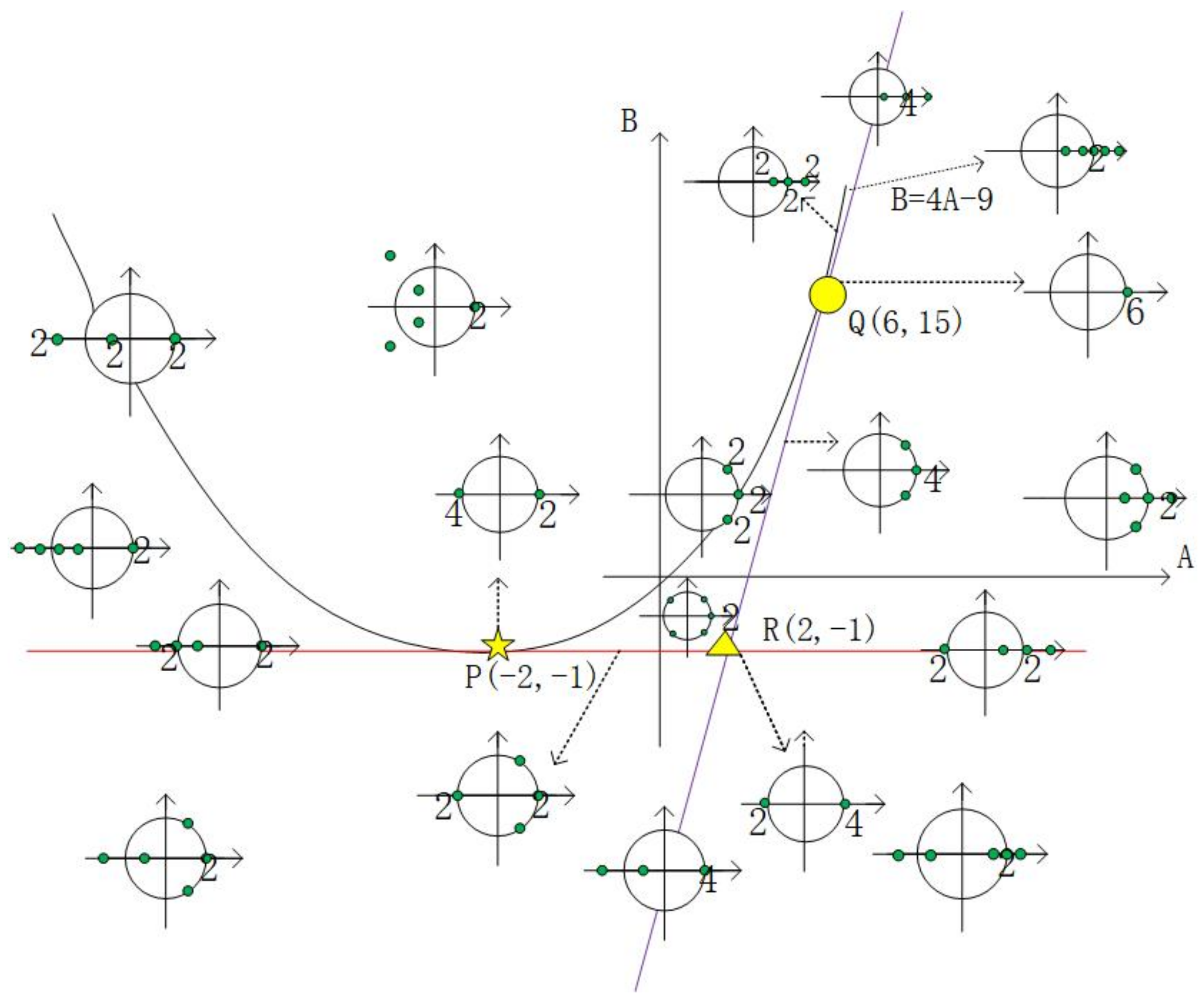
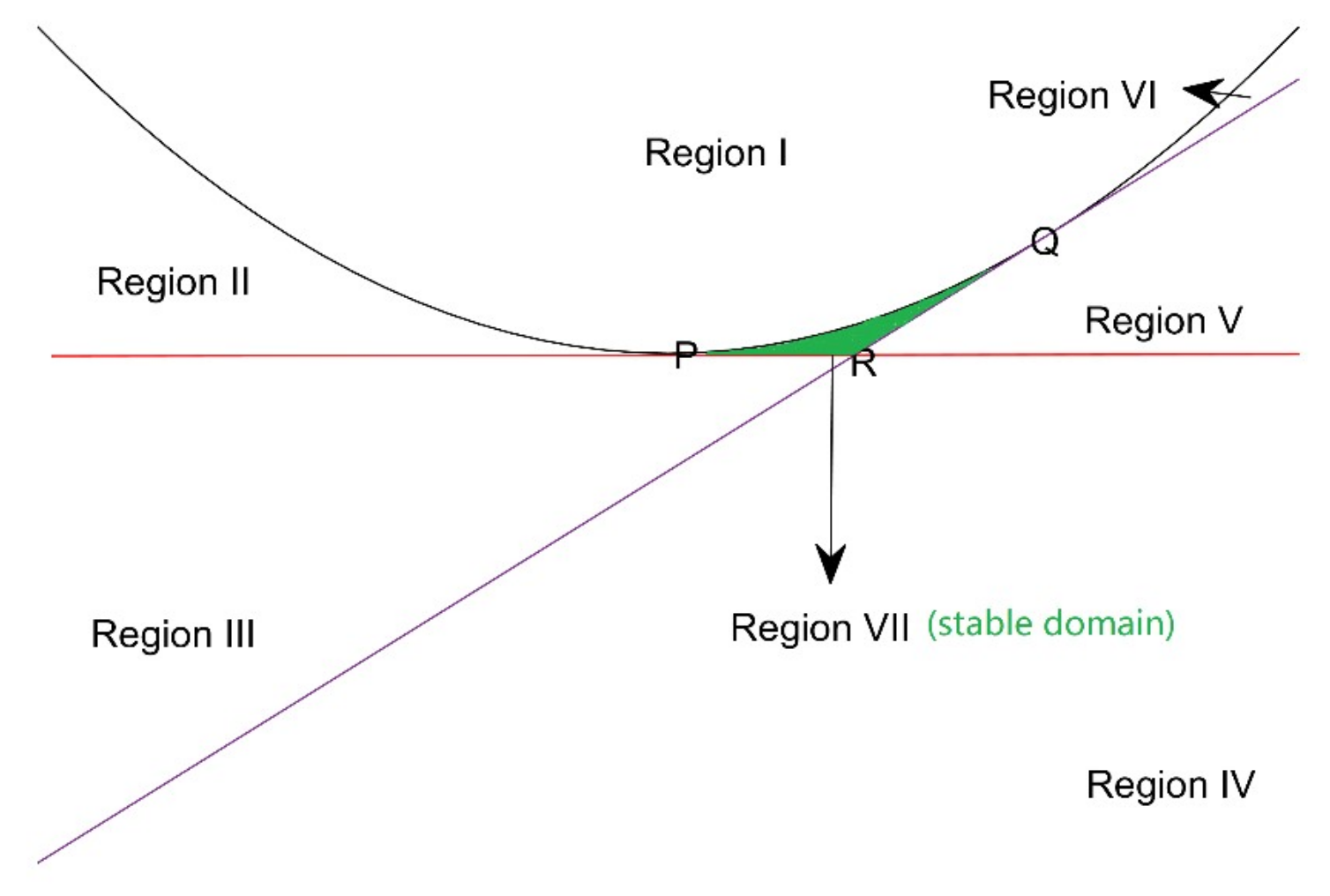
3.3. The Topological Types and Bifurcations of Periodic Orbits in (A, B) Plane

Based on the above discussions, we can obtain three critical curves in the parameter (A, B) plane:

(a)

$B=\frac{A^2}{4}+A$, which corresponds to a parabola in the (A, B) plane;

(b)

$B=4A-9$, which is a straight line tangent to the parabola in (a) at point $Q(6,15)$;

(c)

$B=-1$, which is a horizontal line tangent to the parabola in (a) at its vertex $P(-2,-1).$

Furthermore, the distribution of characteristic multipliers in different regions of the parameter plane (A, B) is plotted in Figure 1. It is noteworthy that a similar picture can be seen in Scheeres [29] and Karydis et al. [34]. However, the parameters plotted in the figures are different. The precise numerical criterion of 13 topological types of periodic orbits is presented in

Table 2. Topological classifications of periodic orbits by the locations of parameters (A, B), the 13 topological cases: P1–P7, PPD1–PPD4, PDRS1, PK1 [25].

Ranges of (A, B)	Locations of (A, B)	Characteristic Multipliers	Topological Cases
$B>\frac{A^2}{4}+A$	region I	1(multiplicity 2), $r^{\pm 1}{e}^{\pm i\theta }(0<r<1,0<\theta <\pi )$	P1
$B<\frac{A^2}{4}+A,A<-2;$ $4A-9<B<\frac{A^2}{4}+A,A>6;$ $B<4A-9,B<-1$	region II, IV and VI	1(multiplicity 2), ${\alpha }^{\pm 1},{\beta }^{\pm 1}(0<|\alpha |<1,0<|\beta |<1,\alpha \ne \beta )$	P3
$(B-4A+9)(B+1)<0$	region III and V	1(multiplicity 2), $e^{\pm i\theta }(0<\theta <\pi )$, ${\alpha }^{\pm 1}(0<|\alpha |<1)$	P4
$max\{4A-9,-1\}<B<\frac{A^2}{4}+A$	region VII	1(multiplicity2), $e^{\pm i{\theta }_k}(0<{\theta }_k<\pi ,k=1,2,{\theta }_1\ne {\theta }_2)$	P2
$B=\frac{A^2}{4}+A,\left|A-2\right|>4$	common boundaries of region I and II, VI and I	1(multiplicity 2), $\alpha$(multiplicity 2, $0<\left|\alpha \right|<1$), ${\alpha }^{-1}$(multiplicity 2)	PDRS1
$B=-1,\left|A\right|>2$	common boundaries of region II and III, IV and V	1(multiplicity 2), −1(multiplicity 2), ${\alpha }^{\pm 1}(0<|\alpha |<1)$	PPD4
$B=4A-9,\left|A-4\right|>2$	common boundary of region III and IV, V and VI	1(multiplicity 4), ${\alpha }^{\pm 1}(0<|\alpha |<1)$	P6
$B=\frac{A^2}{4}+A,\left|A-4\right|<2$	common boundary of region VII and I	1(multiplicity 2), $e^{i\theta }$(multiplicity 2, $0<\theta <\pi$), $e^{-i\theta }$(multiplicity 2)	PK1
$B=-1,\left|A\right|<2$	common boundary of region VII and III	1(multiplicity 2), −1(multiplicity 2), $e^{\pm i\theta }(0<\theta <\pi )$	PPD3
$B=4A-9,\left|A-4\right|<2$	common boundary of region VII and V	1(multiplicity 4), $e^{\pm i\theta }(0<\theta <\pi )$	P5
$B=-1,A=-2$	point P $(-2,-1)$	1(multiplicity 2), −1(multiplicity 4)	PPD2
$B=-1,A=2$	point R $(2,-1)$	1(multiplicity 4), −1(multiplicity 2)	PPD1
$B=15,A=6$	point Q (6, 15)	1(multiplicity 6)	P7

. Here, we use the same notations of topological types as those in the topological classification work of Jiang et al. [25]. One can see that the (A, B) plane is divided into seven domains by these critical curves, which correspond to case P1, case P2, case P3 and case P4. For the convenience of description, the six regions are marked by I–VI from the upper parabola counter-clockwise, while the unique bounded domain with vertexes P, Q and R is labeled region VII in Figure 2. From Figure 1, we can conclude that the stability index $\nu =6$ only when (A, B) belongs to the green region VII in Figure 2. Therefore, a periodic orbit is stable if and only if the corresponding parameter (A, B) lies in region VII. Naturally, we call region VII the stable domain for periodic motions.

When the parameters (A, B) move across common boundaries of the seven regions, bifurcations happen; when (A, B) just touches common boundaries of the seven regions (but does not come across the boundaries), pseudo bifurcations occur. The specific paths of bifurcations can be seen directly from the variation curves of parameters (A, B) on the plane. Possible bifurcation types as parameters (A, B) vary from one region to another are listed in

Table 3. Some bifurcation paths of periodic orbits as parameters (A, B) vary.

Variation Paths of Parameters (A, B)	Bifurcation Types
region I—boundary of I and II—region II,
region VI—boundary of VI and I—region I	real saddle bifurcation
region II—boundary of II and III—region III,
region IV—boundary of IV and V—region V,
region VII—point P—region II,
region VII—boundary of VII and III—region III,
region I—point P—region III	doubling period bifurcation
region III—boundary of III and IV—region IV,
region V—boundary of V and VI—region VI,
region VII—boundary of VII and V—region V,
region VII—point Q—region VI,
region I—point Q—region V	tangent bifurcation
region VII—boundary of VII and I—region I	Neimark–Sacker bifurcation
region III—point R—region V,
region VII—point R—region IV	doubling period bifurcation and tangent bifurcation

. Here, some new bifurcation paths can be obtained such as from region I to point Q, then to region V; from region II to point P, then to region VII; from region I to point P, then to region III; from region III to point R and then to region V; from IV to point R and then to region VII; from region VI to point Q and then to region VII. From a mathematical perspective, these bifurcation types indeed exist. However, it remains to be verified whether a corresponding process exists during numerical continuation of periodic orbits in the potential field of small bodies. These bifurcation paths are shown in Table 3.

For periodic orbits near equilibrium points, Jiang [37] discussed the correspondence relations of topological types of equilibrium points and periodic orbits near equilibrium points. The topological plot in the (A, B) plane, i.e., Figure 1, can give us some new insights. Table 1 illustrates these relations. For equilibrium points belonging to case 1, three periodic orbit families exist, and the corresponding characteristic multipliers are 1, 1, $e^{\pm i{\theta }_k}({\theta }_k\in (0,\pi ),k=1,2)$. Thus, the corresponding (A, B) lies in the stable region, and these periodic orbits are of case P2. For equilibrium points belonging to case 2, two periodic orbit families exist, and the corresponding characteristic multipliers are 1, 1, ${\alpha }^{\pm 1}(\alpha \in (0,1))$, $e^{\pm i\theta }(\theta \in (0,\pi ))$. The corresponding (A, B) lies in region III and V, and these orbits are of case P4. For equilibrium points belonging to case 3, one periodic orbit family exists, and the corresponding characteristic multipliers are 1, 1, ${\alpha }_k^{\pm 1}\left(\right|{\alpha }_k|\in (0,1),k=1,2)$. Therefore, the corresponding (A, B) lies in region II and IV, and these orbits are of case P3. For equilibrium points belonging to case 5, one periodic orbit family exists, and the corresponding characteristic multipliers are 1, 1, ${\alpha }^{\pm 1}\left(\right|\alpha |\in (0,1))$, $r_k^{\pm 1}{e}^{\pm i{\theta }_k}\left(\right|r_k|\in (0,1),{\theta }_k\in (0,\pi ),k=1,2)$. The corresponding (A, B) lies in region I, and these orbits are of case P1. Therefore, the topological information of equilibrium points may illustrate those of periodic orbits near them and vice versa. It is noteworthy that the periodic orbits are very sensitive to parameters near the boundaries of these domains.

4. Applications to Periodic Orbits in the Gravitational Field of Irregular Bodies

As in any other Hamiltonian system, periodic orbits in the potential field of irregular bodies are not isolated but embedded in families. In this section, we will investigate the bifurcation types of periodic orbits of asteroids 101955 Bennu and 2867 Steins during continuation in a family based on previous theory. The outline can be sketched below:

(i)

A hierarchical gridding arithmetic by Yu and Baoyin [22] was applied here for a global search of periodic orbits.

(ii)

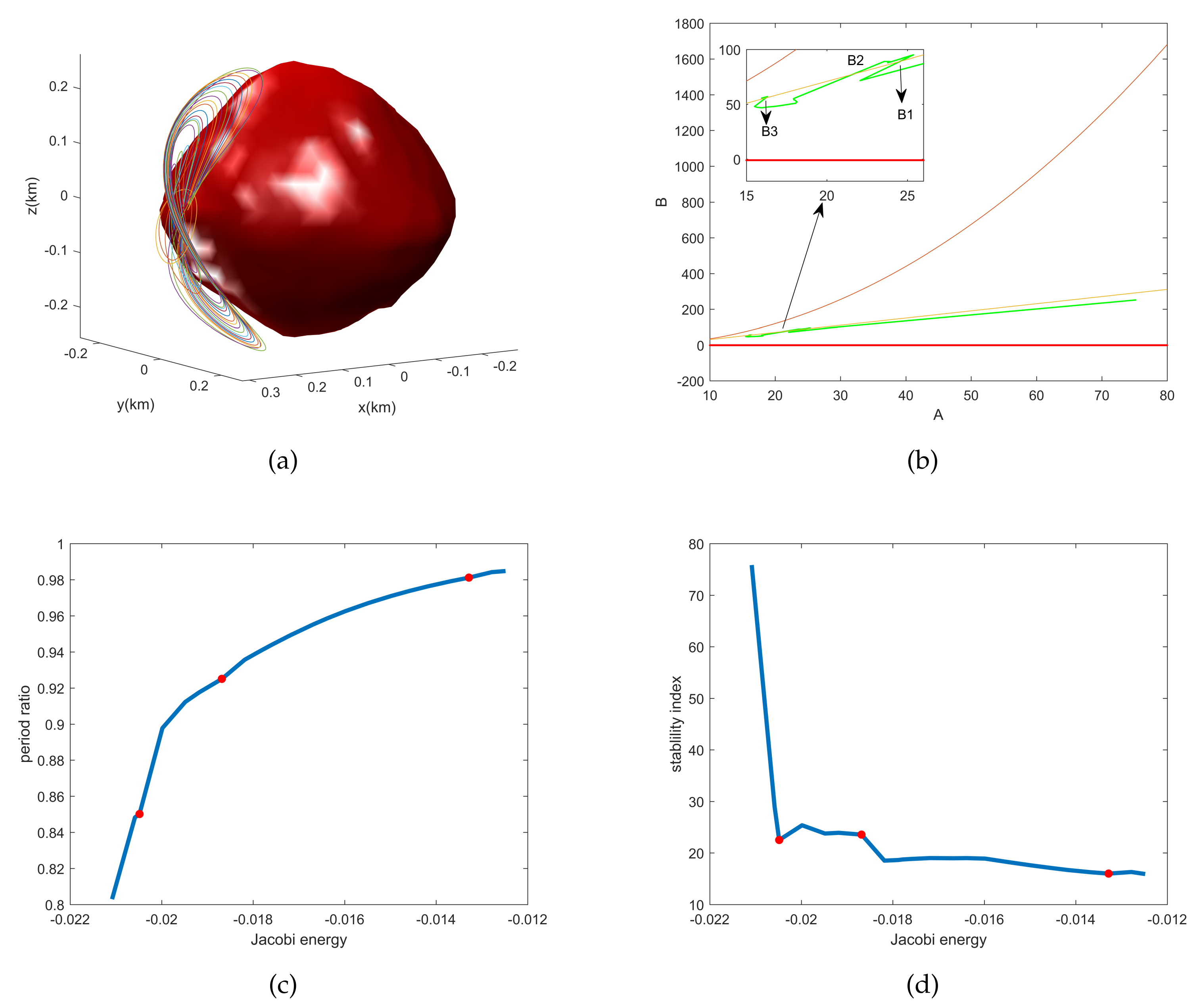
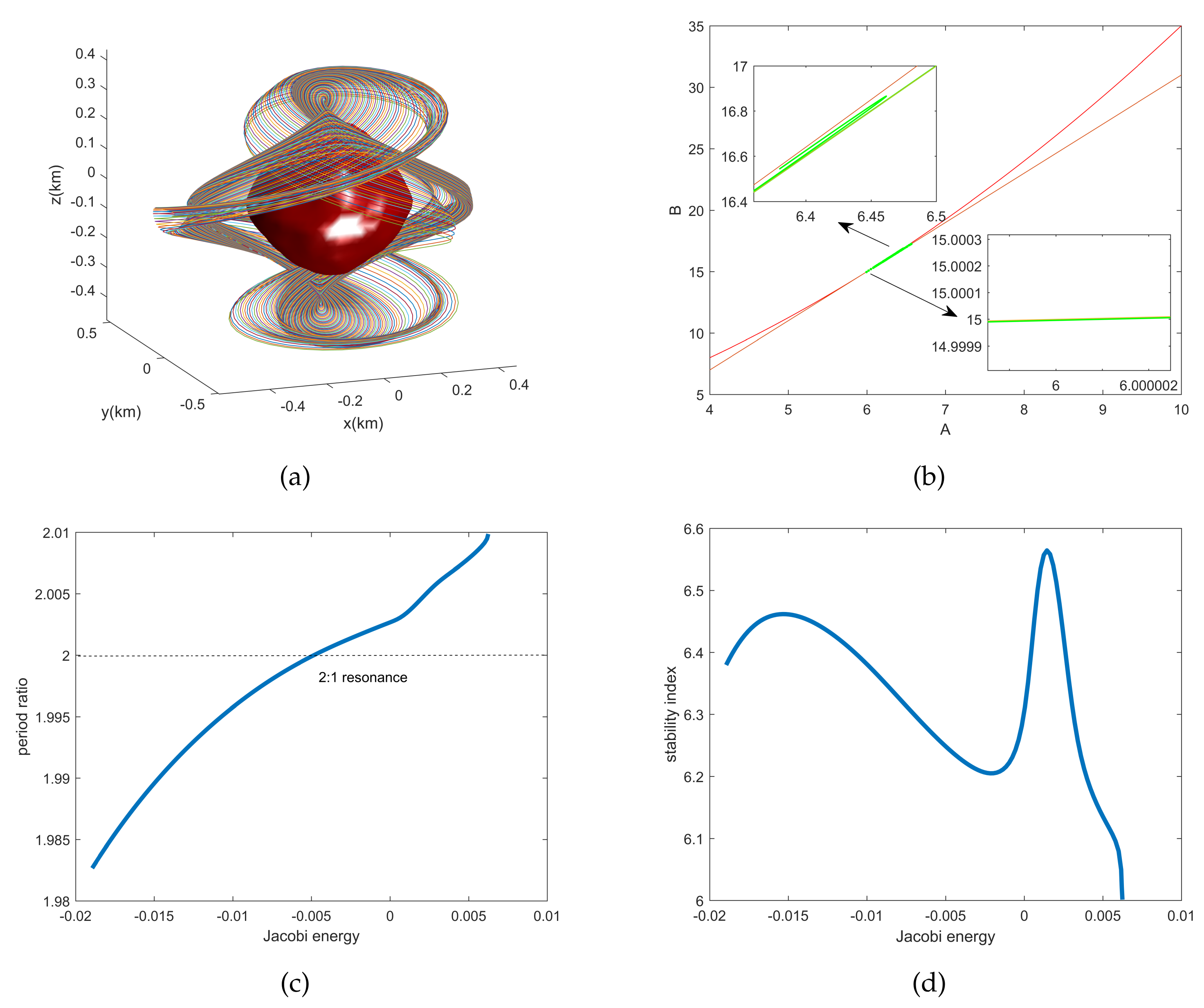
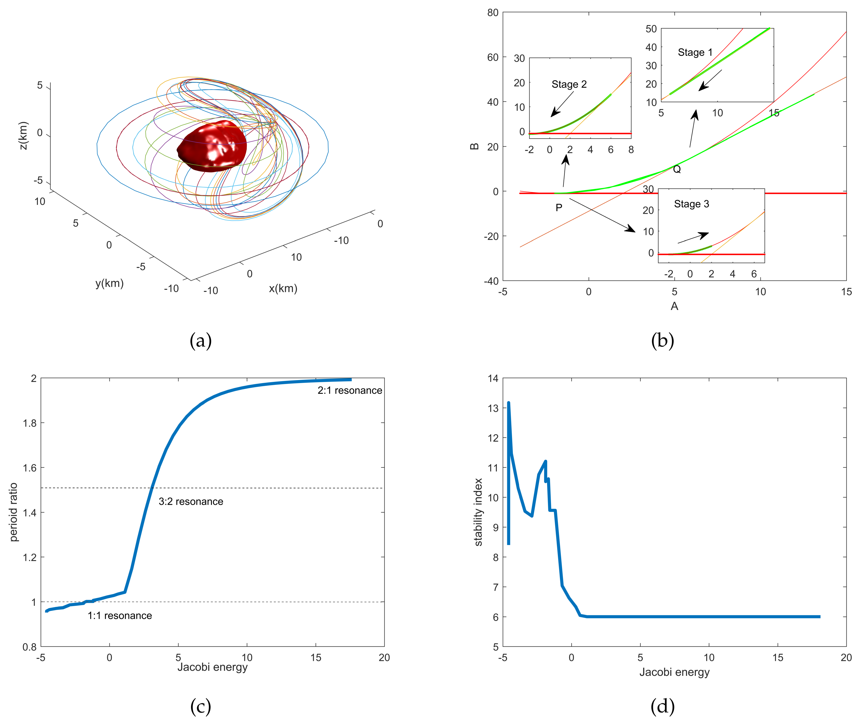
The periodic orbits searched in the former step can be numerically continued into a family by varying the Jacobi energy in appropriate step length. The continuation is conducted in the gradient direction of the energy integral in the phase space.

Generally, the continuation process may stop in three cases: the curve of the orbit intersects with the surface of the body, the Jacobi energy reaches a local minimum or maximum and the orbit converges into an equilibrium point. However, it is also possible that the continuation of a periodic orbit can always be conducted. According to Kang et al. [27], in this case, the periodic orbit will converge to a nearly circular periodic orbit in the equatorial plane with the multiplicity of an integer, and the periodic ratio will converge to that integer.

(iii)

We integrate Equation (5) to find the monodromy matrix for each periodic orbit in a common family. Then, parameters A and B can be easily calculated and plotted in the plane. Thus, the topological types and bifurcations of these orbits can be clearly obtained from the figure.

4.1. Applications to 101955 Bennu

Here, we use asteroid 101955 Bennu to explain the presented theory. Nolan et al. [38] pointed out that the mean diameter is about $492\pm 20$ m. In addition, its density is 0.95 g· cm${}^{-3}$ and the rotation period is 4.288 h. For convenience of calculation, the unit of length here is set to be 566 m, and the time unit is taken as its period. The positions and topological types of relative equilibrium points in the potential field of Bennu were calculated by Wang et al. [36]. According to their results, there exist nine equilibria, namely E1–E9, among which eight equilibria E1–E8 lie outside the asteroid. Moreover, E1, E3, E5, E7 are of topological case 2, while equilibria E2, E4, E6, E8 are of case 5. Lyapunov center theorem guarantees that there exist at least two family periodic orbits around equilibria E1, E3, E5, E7.

In this subsection, we analyze the bifurcations of periodic orbit family emanating from equilibrium point E1. To decrease the possibility of touching the surface of Bennu, we will emphasize on the vertical orbit family V1 around E1. This periodic orbit family is plotted in Figure 3a and the initial conditions at the beginning of continuation can be obtained from

Table 4. Initial conditions and periods of periodic orbit families near 101955 Bennu and 2867 Steins at the beginning of continuation: family V1 and V2 correspond to periodic orbits in Figure 3 and Figure 4, family V3 corresponds to orbits in Figure 5. The data here are normalized.

Periodic Orbit Family	Normalized Period	Initial Position	Initial Velocity
V1	0.802960550501	[0.533051574923, 0.0308716077095, 0.0164503086145]	[−0.0200789540464, −0.884496167760 $\times {10}^{-3}$, 0.649048914541 $\times {10}^{-5}$]
V2	1.98267008174	[0.767915266773, 0.196758690452, −0.158788006313]	[0.995558894975, −2.63610169181, 1.28273214591]
V3	0.951842774046	[0.866022473874, −0.0683721279246, −0.137217733554]	[0.245898975991, 0.141474174266, 0.761661775539]

. One can see that the vertical family near E1 starts with the shape of a small circle; then, the circle becomes increasingly larger and ultimately changes into an orbit with the shape of a figure eight. Figure 3b shows the variation paths in the parameters A and B in the plane. We obtain that (A, B) starts from the region V and enters region VI in a critical case which corresponds to point B1 in the subfigure. During this process, a pair of multipliers on the unit circle collide at point +1, and then two real multipliers are generated from +1. This is a tangent bifurcation. As the Jacobi energy continues to increase, a process opposite to the former happens, which corresponds to point B2 in the subfigure. This is also a tangent bifurcation. Similarly, at a critical situation, a tangent bifurcation happens which corresponds to point B3 in the subfigure. Therefore, we conclude that during continuation from periodic orbit, the geometric shape of the orbit changes from nearly circular to figure eight and the tangent bifurcations happen three times. From Figure 3c,d, we can observe that the period ratio lies in the interval [0.8, 0.99] and the stability index decreases rapidly at the beginning, then increases a little and, finally, decreases very slowly. During this, no simple resonances occur. This implies the instability of these periodic orbits are becoming weaker and weaker in some sense. Here, the continuation stops when the Jacobi energy reaches a local maximum.

Another periodic orbit family V2 with period ratio near 2:1 resonance is presented in Figure 4. One can also obtain the initial conditions from Table 4. The sample of orbits are shown in Figure 4a. Figure 4b illustrates that (A, B) starts from the region VI and moves toward point Q and finally enters region VII in the plane. This means that the topological types of orbits vary from case P3 to P7 and finally to case P2. Namely, two pairs of real multipliers collide at +1 in some critical case. Therefore, the tangent bifurcation happens. From Figure 4c,d, we can observe the variation of period ratios and stability index. It implies that when 2:1 resonance happens, the Jacobi energy is less than −0.005 m${}^2·$ s${}^{-2}$ and the corresponding orbit is unstable. However, when the Jacobi energy is about 0.0065 m${}^2·$ s${}^{-2}$, the orbit is stable.

4.2. Applications to 2867 Steins

According to OSIRIS observations [39,40], 2867 Steins is an E-type asteroid with a bulk density of 1.8 g· cm${}^{-3}$ and a rotation period of 6.04679 h. In this subsection, the length unit for motions in the potential field of 2867 Steins is defined as 6.80653 km and the time unit is 6.04679 h. We choose the vertical periodic orbit with initial conditions in Table 4 to start our continuation. First, numerical continuation in the direction of energy decreasing is conducted. Computation results show that the orbit converges to a point located at $(0.8844,-0.1143,0.0028)$. From the theory of dynamical systems, this point must be an equilibrium point. During this process, the path of (A, B) is included in the interior of region V and no bifurcation occurs. Therefore, we can infer that the equilibrium point is of case 2. In fact, by the results of Wang et al. [36], we can conclude that this point is exactly E1, namely the equilibrium point on the $+x$ axis.

In the following, we analyze the continuation conducted in the direction of energy increasing. Based on the variation paths of (A, B) in the plane in Figure 5b, the continuation process can be divided into three stages. During the first stage, the Jacobi energy is less than 0.316 m${}^2·$ s${}^{-2}$. (A, B) starts from region V, and then transits the common boundary of region V and VI and enters region VI. Then, (A, B) moves toward point Q in region VI. In a critical case, (A, B) reaches the point Q. During the second stage, the Jacobi energy is less than 3.12 m${}^2·$ s${}^{-2}$ and (A, B) moves toward point P in region VII. After that, (A, B) reaches point P. In stage 3, (A, B) leaves point P and moves along the parabola part PQ. Therefore, a tangent bifurcation happens when (A, B) is located at point Q or the common boundary of region V and VI. The topological types of periodic orbits transition from case P4, to case P3, to P7 and then to P2. Moreover, a pseudo doubling period bifurcation happens when they are located at point P. After that, the amplitudes of the periodic orbits on the z-axis decrease, and finally they change into a family of nearly circular orbits. Figure 5c shows that a 3:2 resonance happens and that the corresponding circular orbit is stable. Figure 5d presents the variations of stability index during continuing this period orbit family. We can see when the Jacobi energies are positive, periodic orbits in this family are stable. Here, the continuation process can always go on and the orbits become nearly circular.

5. Conclusions

An investigation of topological types and bifurcations of periodic orbits from a global point of view was conducted in this work. We used the traces of the monodromy matrix and its square matrix as parameters in the plane to illustrate the bifurcation process. Some new paths of bifurcations were discovered. The bifurcations of the vertical periodic orbit family near equilibrium points E1 of 101955 Bennu and 2867 Steins differed greatly. For 101955 Bennu, the continuation stopped when the Jacobi energy reached a local maximum and tangent bifurcations happened three times; for 2867 Steins, the continuation would never stop. Both tangent bifurcations and pseudo period-doubling bifurcations occurred. In addition, the orbits finally varied into nearly circular orbits on the equator. Even though the geometric shapes of periodic orbits remained unchanged, the topological types may vary dramatically. Furthermore, the variations in the period and stability index were studied through numerical methods. Furthermore, the correspondence relations of equilibrium points and associated periodic orbits can be employed as the periodic orbit converges to a point.

Comparing these periodic orbit families, we can obtain some interesting properties. (1) Figure 3c and Figure 4c illustrate that when the Jacobi energy lies in some common interval, for example, [−0.02, −0.014], there exist two different families of periodic orbits. It is well-known that periodic orbits with a fixed value of Jacobi energy are isolated in a generic sense. However, periodic orbits with a fixed value of Jacobi energy may not be unique. This reflects the complexity of the geometry and topology of the energy hypersurface. It would be nice to discuss the relations between periodic orbits with a fixed value of Jacobi energy. (2) As continuing the periodic orbit family emanating from equilibrium points belonging to the same topological type in the potential field of different small bodies, the continuation process and bifurcations may be completely different. One may wonder the topological or geometrical obstacles for the periodic orbit family in Figure 3a converging into the nearly circular orbit.

References

1. Belton, M.; Veverka, J.; Thomas, P.; Helfenstein, P.; Simonelli, D.; Chapman, C.; Davies, M.E.; Greeley, R.; Greenberg, R.; Head, J. Galileo Encounter with 951 Gaspra: First Pictures of an Asteroid. Science 1992, 257, 1647–1652. [Google Scholar] [CrossRef] [PubMed] [Green Version]
2. Scheeres, D.J.; Ostro, S.J.; Hudson, R.S.; Werner, R.A. Orbits Close to Asteroid 4769 Castalia. Icarus 1996, 121, 67–87. [Google Scholar] [CrossRef]
3. Werner, R.A.; Scheeres, D.J. Exterior gravitation of a polyhedron derived and compared with harmonic and mascon gravitation representations of asteroid 4769 Castalia. Celest. Mech. Dyn. Astron. 1996, 65, 313–344. [Google Scholar] [CrossRef]
4. Chanut, T.; Aljbaae, S.; Prado, A.; Carruba, V. Dynamics in the vicinity of (101955) Bennu: Solar radiation pressure effects in equatorial orbits. Mon. Not. R. Astron. Soc. 2017, 470, 2687–2701. [Google Scholar] [CrossRef]
5. Aljbaae, S.; Chanut, T.G.G.; Carruba, V.; Souchay, J.; Prado, A.F.B.A.; Amarante, A. The dynamical environment of asteroid 21 Lutetia according to different internal models. Mon. Not. R. Astron. Soc. 2017, 464, 3552–3560. [Google Scholar] [CrossRef] [Green Version]
6. Aljbaae, S.; Chanut, T.; Prado, A.; Carruba, V.; Hussmann, H.; Souchay, J.; Sanchez, D. Orbital stability near the (87) sylvia system. Mon. Not. R. Astron. Soc. 2019, 486, 2557–2569. [Google Scholar] [CrossRef]
7. Aljbaae, S.; Prado, A.; Sanchez, D.M.; Hussmann, H. Analysis of the orbital stability close to the binary asteroid (90) Antiope. Mon. Not. R. Astron. Soc. 2020, 496, 1645–1654. [Google Scholar] [CrossRef]
8. Jiang, Y. Equilibrium points and orbits around asteroid with the full gravitational potential caused by the 3D irregular shape. Astrodynamics 2018, 2, 361–373. [Google Scholar] [CrossRef] [Green Version]
9. Liu, X.; Baoyin, H.; Ma, X. Equilibria, periodic orbits around equilibria, and heteroclinic connections in the gravity field of a rotating homogeneous cube. Astrophys. Space Sci. 2011, 333, 409–418. [Google Scholar] [CrossRef]
10. Liu, X.; Baoyin, H.; Ma, X. Periodic orbits around areostationary points in the Martian gravity field. Res. Astron. Astrophys. 2012, 12, 551–562. [Google Scholar] [CrossRef] [Green Version]
11. Romanov, V.A.; Doedel, E.J. Periodic Orbits Associated with the Libration Points of the Homogeneous Rotating Gravitating Triaxial Ellipsoid. Int. J. Bifurcat. Chaos 2012, 22, 1230035. [Google Scholar] [CrossRef] [Green Version]
12. Jiang, Y.; Baoyin, H. Periodic Orbits Related to the Equilibrium Points in the Potential of Irregular-shaped Minor Celestial Bodies. Results Phys. 2019, 12, 368–374. [Google Scholar] [CrossRef]
13. Hou, X.; Xin, X.; Feng, J. Forced motions around triangular libration points by solar radiation pressure in a binary asteroid system. Astrodynamics 2020, 4, 17–30. [Google Scholar] [CrossRef]
14. Dichmann, D.J.; Doedel, E.J.; Paffenroth, R.C. The computation of periodic solutions of the 3-body problem using the numerical continuation software auto. In Proceedings of the Libration Point Orbits & Applications—The Conference, Aiguablava, Spain, 10–14 June 2002; pp. 429–488. [Google Scholar]
15. Parker, J.S.; Lo, M.W. Unstable Resonant Orbits near Earth and Their Applications in Planetary Missions. In Proceedings of the AIAA/AAS Astrodynamics Specialist Conference & Exhibit, Providence, RI, USA, 16–19 August 2004. [Google Scholar]
16. Jiang, Y.; Schmidt, J.; Li, H.; Liu, X.; Yang, Y. Stable periodic orbits for spacecraft around minor celestial bodies. Astrodynamics 2018, 2, 69–86. [Google Scholar] [CrossRef] [Green Version]
17. Lian, Y. On the dynamics and control of the Sun—Earth L2 tetrahedral formation. Astrodynamics 2021, 5, 331–346. [Google Scholar] [CrossRef]
18. Eros, A.; Elipe, A. A Simple Model for the Chaotic Motion Around (433) Eros. J. Astronaut. Sci. 2004, 51, 391–404. [Google Scholar]
19. Sanchez, A.; Guedan, A. Nonlinear Stability Under a Logarithmic Gravity Field. Int. Math. J. 2003, 3, 435–453. [Google Scholar]
20. Shang, H.; Wu, X.; Cui, P. Periodic orbits in the doubly synchronous binary asteroid systems and their applications in space missions. Astrophys. Space Sci. 2015, 355, 69–87. [Google Scholar] [CrossRef]
21. Shang, H.; Wu, X.; Qin, X.; Qiao, D. Periodic motion near non-principal-axis rotation asteroids. Mon. Not. R. Astron. Soc. 2017, 471, 3234–3244. [Google Scholar] [CrossRef]
22. Yu, Y.; Baoyin, H. Generating families of 3D periodic orbits about asteroids. Mon. Not. R. Astron. Soc. 2012, 427, 872–881. [Google Scholar] [CrossRef] [Green Version]
23. Yu, Y.; Baoyin, H.; Jiang, Y. Constructing the natural families of periodic orbits near irregular bodies. Mon. Not. R. Astron. Soc. 2015, 453, 3269–3277. [Google Scholar] [CrossRef]
24. Jiang, Y.; Baoyin, H.; Li, J.; Li, H. Orbits and manifolds near the equilibrium points around a rotating asteroid. Astrophys. Space Sci. 2014, 349, 83–106. [Google Scholar] [CrossRef] [Green Version]
25. Jiang, Y.; Yu, Y.; Baoyin, H. Topological Classifications and Bifurcations of Periodic Orbits in the Potential Field of Highly Irregular-shaped Celestial Bodies. Nonlinear. Dyn. 2015, 81, 119–140. [Google Scholar] [CrossRef] [Green Version]
26. Lan, L.; Ni, Y.; Jiang, Y.; Li, J. Motion of the moonlet in the binary system 243 Ida. Acta Mech. Sin. 2018, 34, 214–224. [Google Scholar] [CrossRef]
27. Kang, H.; Jiang, Y.; Li, H. Convergence of a periodic orbit family close to asteroids during a continuation. Results Phys. 2020, 19, 103353. [Google Scholar] [CrossRef]
28. Zeng, X.; Alfriend, K. Periodic orbits in the Chermnykh problem. Astrodynamics 2017, 1, 41–55. [Google Scholar] [CrossRef]
29. Scheeres, D. Orbital Motion in Strongly Perturbed Environments; Springer: Berlin/Heidelberg, Germany, 2012. [Google Scholar]
30. Broucke, R. Stability of periodic orbits in the elliptic restricted three-body problem. AIAA J. 1969, 7, 1003–1009. [Google Scholar] [CrossRef]
31. Zagouras, C.; Markellos, V.V. Axisymmetric periodic orbits of the restricted problem in three dimensions. Astron. Astrophys. 1977, 59, 79–89. [Google Scholar]
32. Papadakis, K.E.; Zagouras, C.G. Bifurcation points and intersections of families of periodic orbits in the three-dimensional restricted three-body problem. Astrophys. Space Sci. 1993, 199, 241–256. [Google Scholar] [CrossRef]
33. Kalantonis, V.S. Numerical Investigation for Periodic Orbits in the Hill Three-Body Problem. Universe 2020, 6, 72. [Google Scholar] [CrossRef]
34. Karydis, D.; Voyatzis, G.; Tsiganis, K. A continuation approach for computing periodic orbits around irregular-shaped asteroids. An application to 433 Eros. Adv. Space Res. 2021, 68, 4418–4433. [Google Scholar] [CrossRef]
35. Jiang, Y.; Baoyin, H. Orbital Mechanics near a Rotating Asteroid. J. Astrophys. Astron. 2014, 35, 17–38. [Google Scholar] [CrossRef]
36. Wang, X.; Jiang, Y.; Gong, S. Analysis of the Potential Field and Equilibrium Points of Irregular-shaped Minor Celestial Bodies. Astrophys. Space Sci. 2014, 353, 105–121. [Google Scholar] [CrossRef] [Green Version]
37. Jiang, Y. Equilibrium Points and Periodic Orbits in the Vicinity of Asteroids with an Application to 216 Kleopatra. Earth Moon Planets 2015, 115, 31–44. [Google Scholar] [CrossRef]
38. Nolan, M.C.; Magri, C.; Howell, E.S.; Benner, L.; Giorgini, J.D.; Hergenrother, C.W.; Hudson, R.S.; Lauretta, D.S.; Margot, J.L.; Ostro, S.J. Shape model and surface properties of the OSIRIS-REx target Asteroid (101955) Bennu from radar and lightcurve observations. Icarus 2013, 226, 629–640. [Google Scholar] [CrossRef] [Green Version]
39. Keller, H.U.; Barbieri, C.; Koschny, D.; Lamy, P.; Vernazza, P. E-type asteroid (2867) Steins as imaged by OSIRIS on board Rosetta. Science 2010, 327, 190–193. [Google Scholar] [CrossRef]
40. Jorda, L.; Lamy, P.L.; Gaskell, R.W.; Kaasalainen, M.; Groussin, O.; Besse, S.; Faury, G. Asteroid (2867) Steins: Shape, topography and global physical properties from OSIRIS observations. Icarus 2012, 221, 1089–1100. [Google Scholar] [CrossRef]
Figure 1. Topological types of periodic orbits in the plane of parameters: the green point in each subfigure represents a multiplier, and the number near the point is its multiplicity.
Aerospace 09 00151 g001
Figure 2. The distribution of seven regions in the plane of parameters (A, B).
Aerospace 09 00151 g002
Figure 3. Periodic orbits during the continuation process of the vertical orbits family near 101955 Bennu: (a) sample of orbits in the rotating coordinate, (b) variation paths of (A, B) in the plane, (c) the variation of period ratios during continuation, (d) the variation of stability index with respect to the Jacobi energy. The unit for the Jacobi energy is m 2 · s 2 . The three red points marked in (c,d) correspond to bifurcations and their Jacobi constants are 0.0204 , 0.0187 , 0.0133 .
Aerospace 09 00151 g003
Figure 4. Periodic orbits during the continuation process of the 2:1 resonant family near 101955 Bennu: (a) sample of orbits in the rotating coordinate, (b) variation paths of (A, B) in the plane, (c) the variation of period ratios during continuation, (d) the variation of stability index with respect to the Jacobi energy. The unit for the Jacobi energy is m 2 · s 2 .
Aerospace 09 00151 g004
Figure 5. Periodic orbits during the continuation process of the vertical orbits family near 2867 Steins: (a) sample of orbits in the rotating coordinate, (b) variation paths of (A, B) in the plane, (c) the variation of period ratios during continuation, (d) the variation of stability index with respect to the Jacobi energy. The unit for the Jacobi energy is m 2 · s 2 .
Aerospace 09 00151 g005