Subarea Description and Breakage Constitutive Model of Rock Mass Based on CT Test

Abstract

Based on CT experiments of the mechanical behavior of a certain sandstone, the safety zone, the damaging zone, and the fracture zone of geotechnical materials were defined, and the CT threshold standard of this zone was discussed and empirically selected. Mathematical morphological image measurement technology was used to analyze the CT information of each section, and the variation law of the sandstone CT number with the loading process and the conditions of the damaging zone was studied. According to the statistical results of the CT number of the safety zone, the damaging zone, and the fracture zone obtained at each loading stage, a statistical-damage variable based on the CT number was defined, and the equation of the damage evolution pertinent to this damage variable was established. On the basis of all these data, a constitutive model that can reflect the divisional damage-fracture of sandstone was constructed. The theoretical stress–strain curve and the measured curve were well fitted, demonstrating that the improved constitutive model could accurately reflect the failure of sandstone partitions. A qualitative analysis of CT scans and a quantitative analysis of the constitutive model were combined in this experiment, which has a certain reference value for the development of geotechnical engineering experiments.

1. Introduction

Computed tomography (CT) technology is a widely used radiographic imaging technique that provides high-resolution digital images [1]. As a nondestructive testing technology, CT technology has the advantages of the dynamic, quantitative, and nondestructive measurement of the internal structural changes of geotechnical materials during the stress process. This provides the possibility for the mesoscopic study of rock and soil masses [2,3].

For a long time, people have been using CT technology for related geotechnical studies [4,5,6,7,8]. Sun et al. [4] applied CT technology to the field of geotechnical engineering to study the progressive fracture of a soil–rock mixture under uniaxial compression. It was observed that small cracks gradually accumulated during the elastic-deformation stage, and eventually formed visible cracks during the plastic-deformation stage. Mcbeck et al. [5] used CT techniques to analyze and study the propagating fractures and permeability-force chains in porous granular rocks, and they predicted how porosity controls the persistence of stress fields. Zaima and Katayama [6] used CT technology to analyze the evolution of the elastic-wave velocity and amplitude during the triaxial deformation of granite, and they established a systematic relationship between the elastic-wave velocity, amplitude, fracture development, and fluid saturation. Zhang et al. [7] used CT technology to study the damage process of concrete and observed the formation process of cracks. Yang [8] used micro-CT-scanning technology to observe the fracturing mechanism and failure characteristics of compressed hollow sandstone under different pressures. These people have recognized the inadequacies brought about by the homogenization of local problems, and the experiments were more qualitative than quantitative [9,10,11,12,13,14,15,16,17].

In geomechanics, different constitutive models are established according to the physical properties of different materials [18,19,20,21,22]. Wang et al. [18] established a constitutive model for cohesive soil research considering soil–structure interactions. By analyzing the dynamic hysteretic constitutive model of cohesive soil, the fitting equation of the dynamic shear modulus and the damping ratio of soil were proposed. Hirai et al. [19] established an elastic–plastic constitutive model based on the characteristics of expansion-buffer material for research. It was concluded that, in the case of compacted bentonite materials, the nonlinear behavior in the consolidation test was more pronounced than that of ordinary clay materials. Nikolinakou and Whittle [20] established a constitutive model to study the structural changes and dilatation behavior of old alluvial. It provided a framework to explain how the engineering properties of old-alluvial-soil profiles varied vertically with the weathering state. Deng et al. [21] developed a constitutive model to study the tissue behavior of uniaxial cyclic tension hybrid fiber-reinforced concrete. It was concluded that adding an appropriate volume content of polypropylene fibers could improve the deformation and energy consumption of the matrix. Guo et al. [22] also established a constitutive model to study the plastic-flow behavior of GCr15 steel. It was concluded that the maximum stress decreased with increasing temperature, and it increased with an increasing strain rate. These people established the constitutive models required for quantitative analysis based on experimental samples, but these have rarely been combined with CT experiments [9,12,13,14,15,23,24,25,26,27,28,29,30].

Based on the combination of CT and a constitutive model, a CT test was carried out on the mechanical properties of a sandstone, and the test results were obtained [31,32]. According to the theory of partition description, the safety zone, the damaging zone, and the fracture zone of geotechnical materials were defined, and a quantitative-description system of measurement and statistical modeling was proposed to realize the partition description of the test results under the same standard. The CT-number information attached to the partition results was detected and statistically analyzed. According to the defined statistical-damage variables, the damage-evolution equation and CT-number-based constitutive equation were established, and on this basis, the constitutive model reflecting the damage in the sandstone area was established [33].

2. Subarea Description Theory

The traditional global-statistical-analysis method will make the locally weakened information evenly distributed to the overall level, which is not conducive to exploring the essence of the problem from a mesoscopic perspective [2,4,5,6,7,34,35,36]. In order to discuss the problem from a microscopic point of view, subarea description theory, based on CT-number information within a certain range, was proposed. It was necessary to define the ROI (region of interest). The collection of CT numbers on the cracks in the CT-scan image was used as the region of interest (ROI).

According to the degree of the deterioration of the material properties, the loading process could be divided into three stages: the elastic-deformation stage (including compaction stage), the inelastic-deformation stage, in which cracks were generated and stably propagated, and the crack-penetration-failure stage. When the sample failed, every point in the material (especially the CT cell) went through the entire loading phase. The degree of damage could be divided into three types of damage: no irrecoverable damage, completely irreversible damage, and irreversible damage. Points with similar properties were divided into three point sets: the safe area, damaging area, and fracture area. The collections were defined as follows:

When $H>H_e$, (Equation (1)), it was determined that the material at this point was in a safe state, and the set of all points in a safe state was called the safe zone.

When $H_d<H\le H_e$, it was determined that the material damage at this point was in progress, and the set of all points in the damage-progressing state was called the damaging zone.

When $H\le H_d$ (Equation (2)), it was determined that the material at this point had been damaged, and the set of all points in the damaged state was called the fracture zone.

In the formula, the CT number thresholds H_e and H_d used for the ensemble segmentation were material constants. In practical applications, because the change in the CT number at a certain point was disturbed too much by uncertain factors and it was difficult to track, it was necessary to include points with similar properties into the same set for the partition description. The subarea thresholds used in the article were the transition thresholds from the safe zone to the damaging zone, and from the damaging zone to the fracture zone. Here, the subarea standards H_e and H_d were defined as follows:

$$H_{ei}=\overline{H_{\sigma i}}-{\xi }_1$$

(1)

$$H_{di}=\overline{H_{\sigma i}}-{\xi }_2$$

(2)

In the formula, $H_{ei}$ is the partition threshold of the safety zone in a certain loading stage, $\overline{H_{\sigma i}}$ is the average value of CT numbers in the ROI of the cross-section under a certain loading stage, and ${\xi }_1$ and ${\xi }_1$ are experimental constants.

Due to the initial damage to the rock, it was difficult to track the CT number of a single point and the acquisition error was large, and so the partition operation based on the absolute CT number of a single point was difficult to achieve. The CT image of the selected five sections in each loading stage, and its initial scan, were subjected to an image-difference calculation to reflect the change in the CT number before and after loading and its spatial distribution.

3. Experiment Introduction

The sample sand19 was collected from Shuangcha River, Yaoxian County, Shaanxi Province. After many comparative tests in the early stage, it was found that the samples collected here were Permian feldspar fine sandstones with cemented properties, which were suitable for this test. The bulk density was 26.36 KN/m³, and the water content was 0.25%. The samples were first cleaned and dematerialized, and they were then processed by a rock-sample drilling machine. The sample-processing specifications were 50 mm in diameter and 100 mm in height. After the sample was shortened by 10 mm up and down, a scanning section was selected every 20 mm, and a total of five scanning sections were selected.

The spatial resolution of the CT machine in this experiment was 0.35 mm × 0.35 mm. The minimum identifiable volume was 0.12 mm³ (layer thickness of 1 mm). The density-contrast resolution was 0.3% (2.5 Hu). The scanning voltage of the CT machine was 137 KV. The sweep current was 220 mA. The scan time was 2 s. The layer thickness was 2 mm. The magnification factor was 6.0.

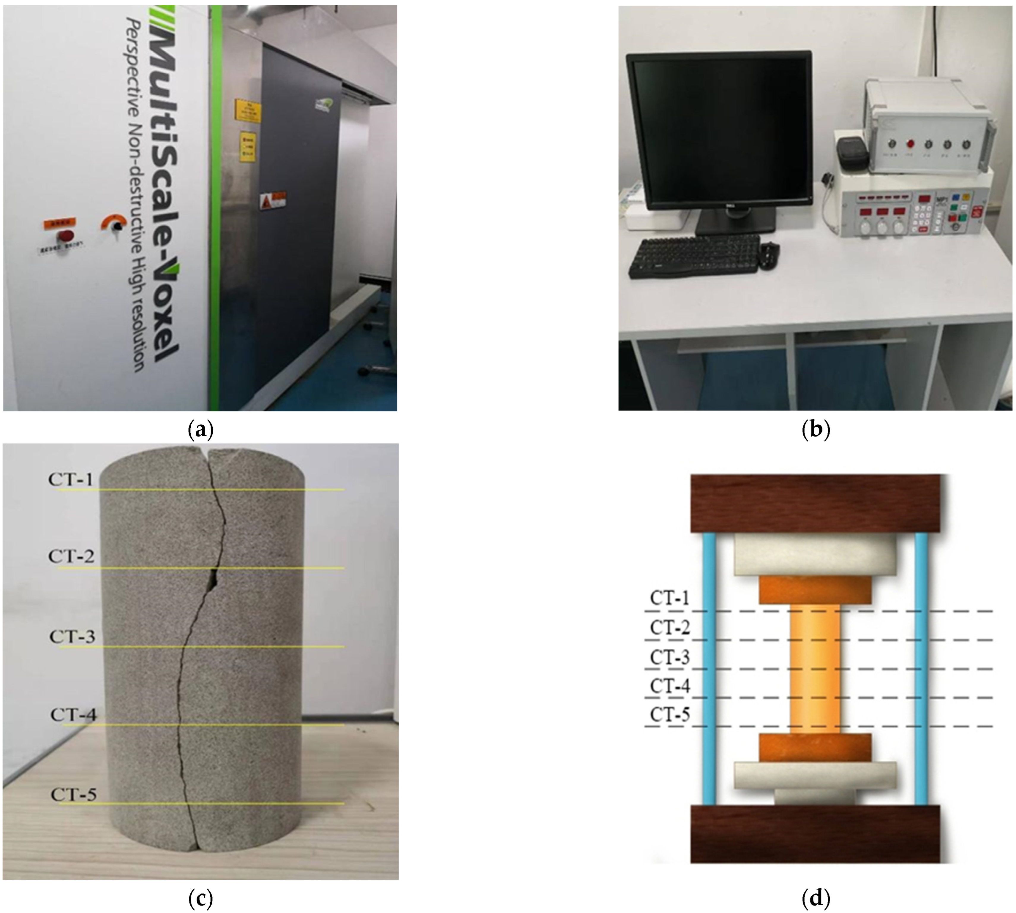
The rock samples were first loaded into the triaxial pressure chamber and sent to the scanning space by the CT bed without confining pressure. The first scan was performed when the specimen was unstressed, and then the axial compression was gradually applied, loaded in stages. The average loading rate was 7.29 × 10⁻³ MPa/s. During each scan, the axial pressure was fixed, and the scan was divided into 5 layers with an interval of 2 cm. The test was stopped when the rock sample was damaged. The test result was a grayscale image stored in 8 digits, the image matrix size was 512 × 512, the image resolution size was 0.15 mm, and each pixel was accompanied by a CT number stored in 12 digits. Laboratory CT-Scan samples and equipment are shown in Figure 1 below.

4. Test Results

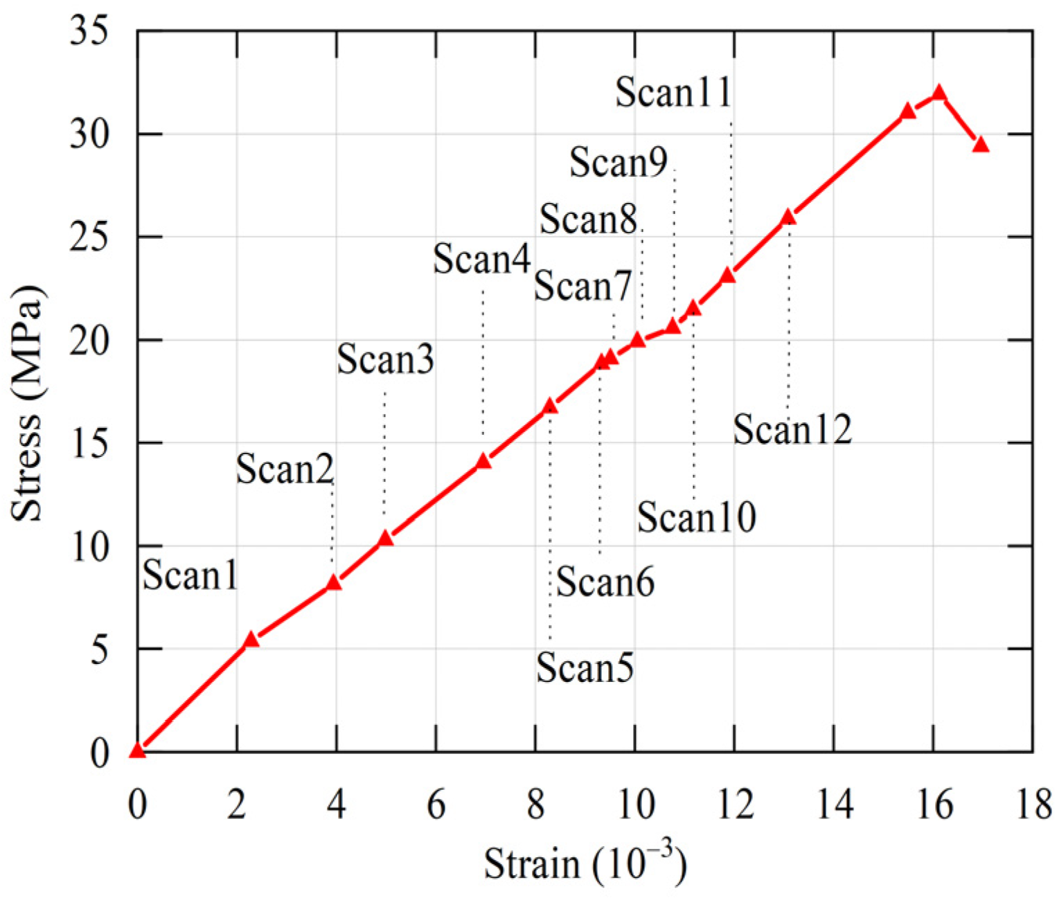
There were five scanning sections in the sample. The stress–strain relationship of sandstone under uniaxial compression was obtained by scanning each section 12 times at different loading stages. A total of 60 CT scans were performed. For each scan, three samples were prepared for testing. The relationship between the specific loading process and scanning is shown in Figure 2 below.

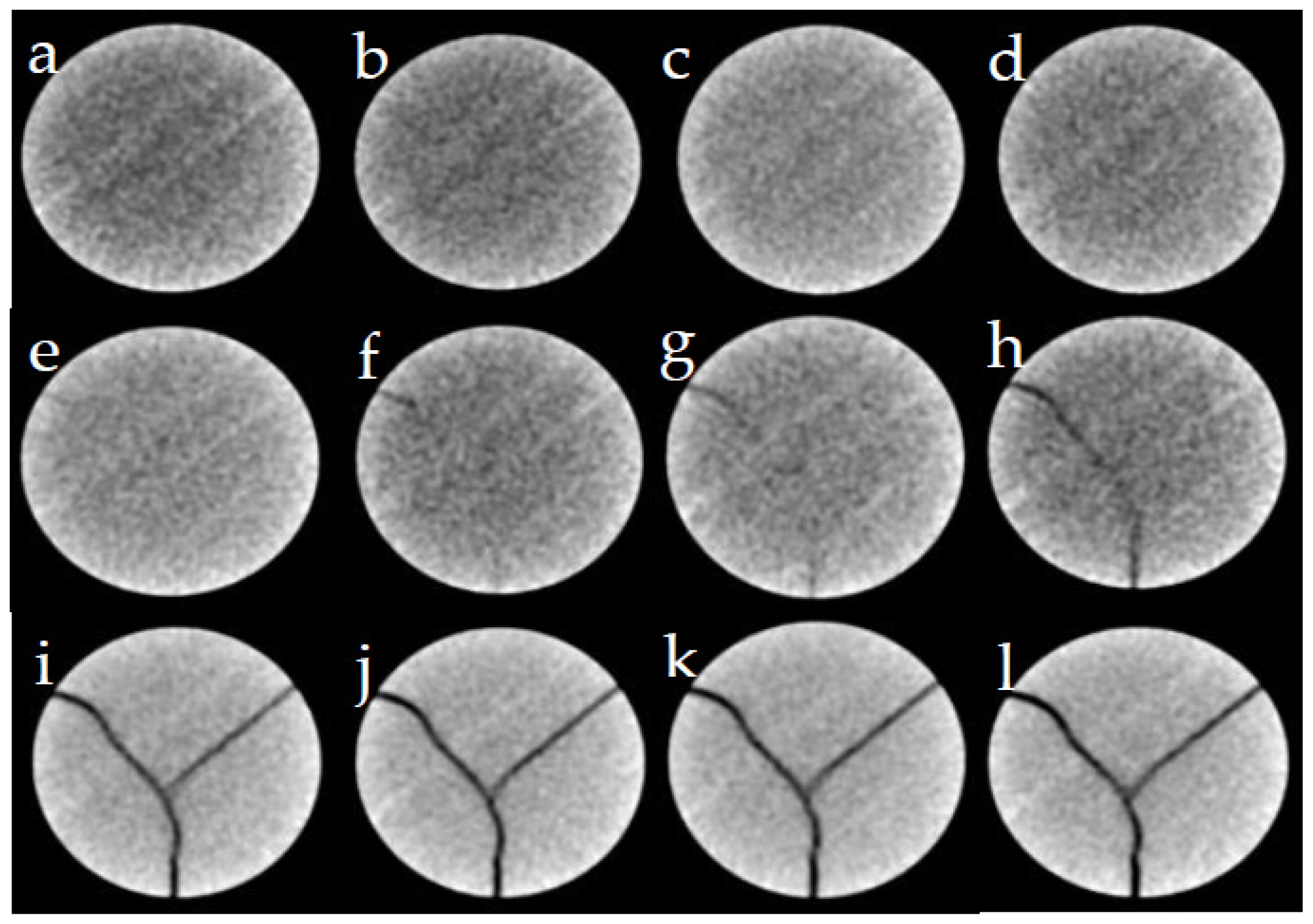
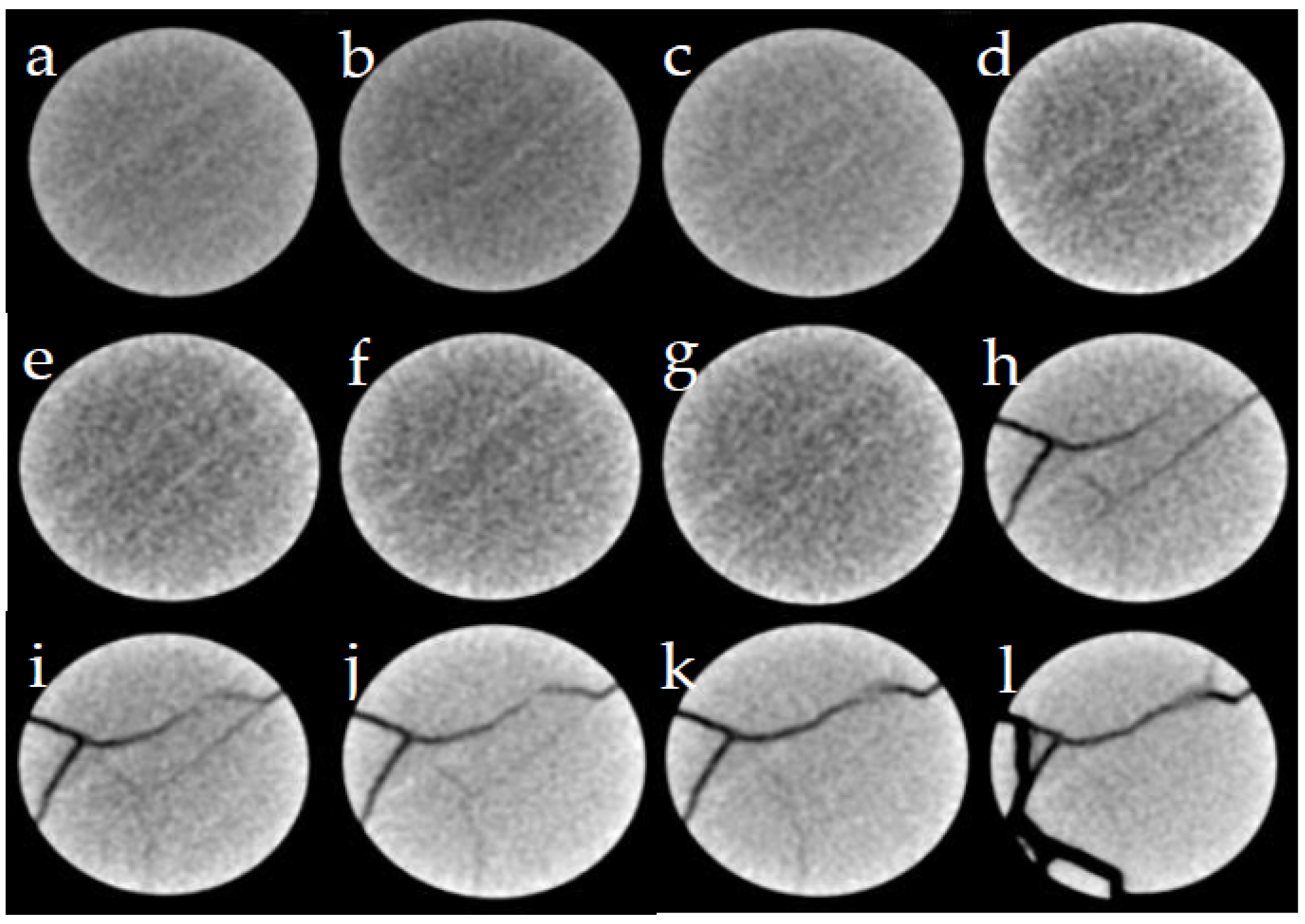
Digital images of 12 loading stages for 3 of the 5 scan sections are shown in the article. CT images of the first scan section are shown in Figure 3.

It can be seen from Figure 3 of the CT-scan images of the first scanning section at each stage that cracks appeared in the scan images when σ = 18.85 MPa, and no cracks were found in the scan results of the previous stages. When σ = 19.09 MPa~25.88 MPa, the cracks grew steadily, and they finally penetrated in each scanning stage.

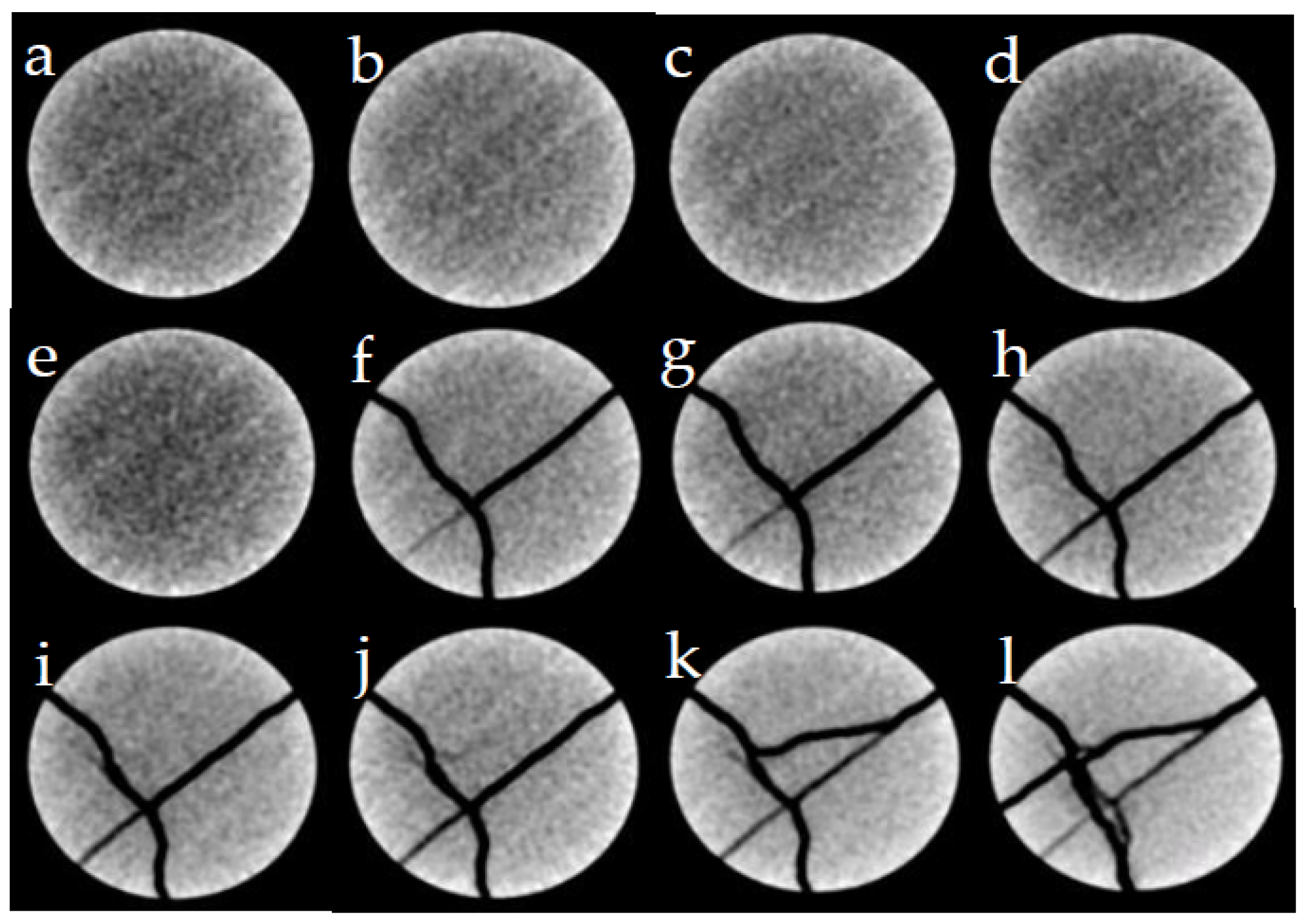
It can be seen from the CT scanning images of the third scanning section in Figure 4 that the cracks only appeared when σ = 18.85 MPa, and then the time for the cracks to propagate to the final penetration was short and very sudden. When σ = 23.05 MPa~25.88 MPa, there were secondary cracks. This section lagged behind the cracks of the first two sections by two loading stages, indicating that the cracks gradually expanded from top to bottom.

It can be seen from the CT-scan images of the fifth scanning section at each stage in Figure 5 that the crack appeared at σ = 19.93 MPa, and then the crack gradually expanded and finally penetrated. Compared with the cracks in the first scanning section, the appearance of the cracks was delayed by 2~3 loading stages, indicating that the cracks gradually expanded from top to bottom. The crack propagation of this section was stable and typical, and this section was specially selected for subsequent analysis and research work.

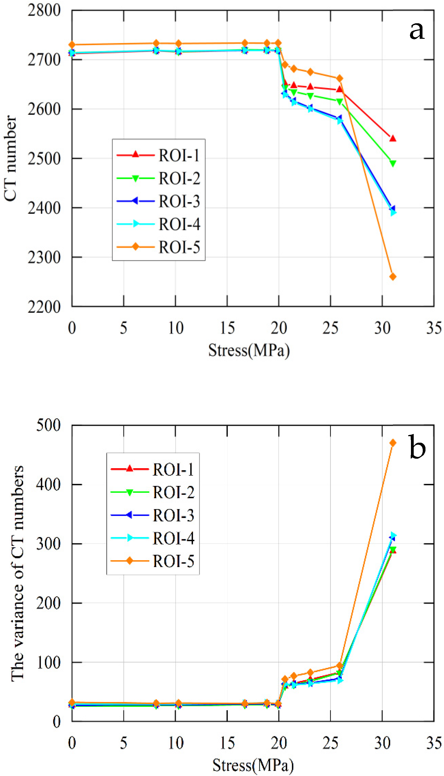
In addition, the variation in the CT number and the variance with stress in the ROI were also studied, as shown in Figure 6.

By analyzing the variation curve of the CT number and the variance of CT numbers with stress in the ROI, it could be seen that when σ = 18.85 MPa or so, the variance curve of the CT number and the variance in the CT numbers of each section began to show an inflection point, but the change was slow. This showed that there were cracks in the section at this time, but the cracks developed slowly. When σ = 25.88 MPa or so, the variance curve of the CT number and the variance in the CT numbers of each section began to change drastically. This showed that the cracks in the section rapidly expanded until they penetrated. The curve-analysis results were roughly consistent with the CT-image observations.

5. Test Analysis

5.1. Threshold Selection

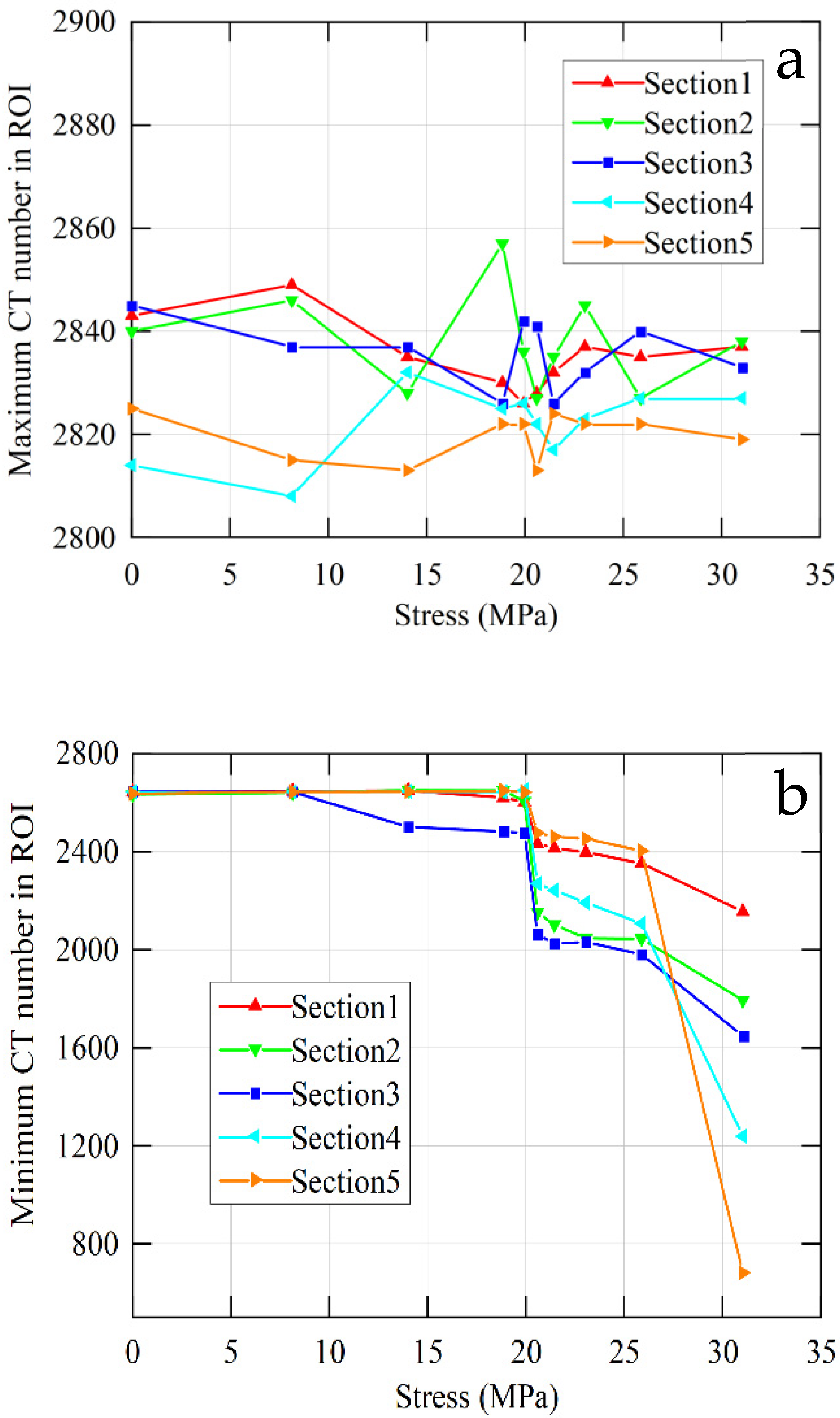
According to the experimental results, the thresholds ${\xi }_1$ and ${\xi }_2$ could be determined. Moreover, ${\xi }_1$ and ${\xi }_2$ were experimental constants, and their accurate selection depended on the development of quantitative CT, a large number of material experiments, and a statistical analysis of the experimental data. Here, empirical values were used [4,5,6,7,8]. The statistical domain used was the ROI, including 86,549 pixels. The relationship curve between the maximum and minimum CT numbers and the stress is presented in Figure 7.

Relatively speaking, the region with the largest CT number represents the better part of the sample, while the region with the minimum value represents the relatively weak part. The relevant data are listed in

Table 1. The maximum CT numbers in the ROI.

Section	Maximum CT Number	Maximum Amplitude
1	2826–2849	23
2	2827–2857	30
3	2826–2845	19
4	2808–2832	24
5	2808–2825	17

.

Because CT numbers are generally stored in 12-bit format, the Hounsfield scale has a total of 4096 levels. The density-contrast resolution of the CT machine used this time was 0.3%, and so the density-contrast error in the range of 4096 was 12.288 Hu. Within this error range, the maximum value fluctuates randomly up and down, there was no monotonic trend, and its properties could be considered unchanged. It could be seen from the above analysis that the maximum value of the CT number did not change much in the whole loading stage, the average amplitude was 22.6, which was a random change, and there was no monotonic trend. It also showed that, regardless of the overall damage of the sample, the sample contained nondestructive or irrecoverable damaged parts.

It can be seen from

Table 2. The minimum CT numbers in the ROI.

Section	Minimum CT Number	Minimum Amplitude
1	2603–2649	46
2	2605–2651	46
3	2476–2645	169
4	2644–2651	7
5	2638–2651	13

that the overall fluctuation in the minimum value in the stress stage was not large, and the amplitude did not exceed 50, but there was no monotonic trend. Only the third segment changed from the other segments, with damage and rupture appearing earlier.

Because the minimum and maximum values did not have a monotonic trend, it could be considered that the microdamage was not enough to change the overall properties of the material and could be used as the segmentation threshold of the safe area. The average amplitude of the maximum value was 22.6, and the amplitude of the minimum value did not exceed 50. When the minimum value changed to a hundredth level, the minimum value showed a monotonous trend, indicating that the occurrence of cracks and stable growth could be used as the threshold for the damage-progress zone, and the segmentation threshold of the damaged zone, which was ${\xi }_1$ = 50, ${\xi }_2$ = 100, was selected.

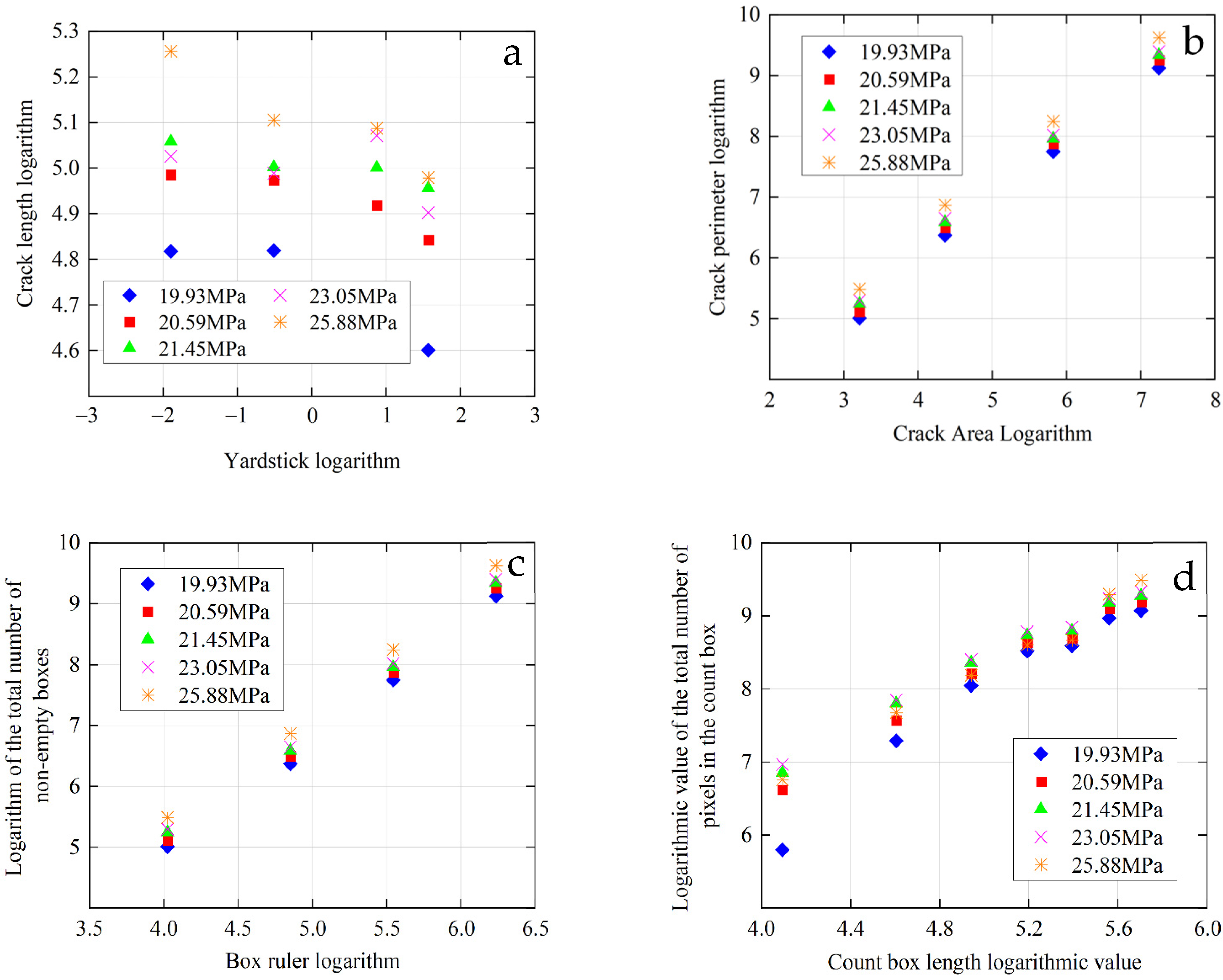
5.2. Application and Analysis of Fractal Dimension

In order to quantitatively describe the degree of “irregularity” in the CT number, it was expanded from integers to fractions for analysis [10,12,13,14,15,16,37]. Under the five loading stages (σ = 19.93 MPa, σ = 20.59 MPa, σ = 21.45 MPa, σ = 23.05 MPa, and σ = 25.88 MPa), the crack images of the third scan section were selected to calculate the fractal dimension using the yardstick logarithmic method, the island method, the box-counting method, and the sandbox method, respectively. The results are shown in Figure 8.

The evolution law of crack fractal dimension could reflect the evolution law of material damage. The development and evolution of the cracks showed good statistical self-similarity and satisfied the scale invariance, which fully indicated that the mesoscopic cracks had fractal characteristics at different loading stages.

It can be seen from

Table 3. Computing results of fractal dimension under each loading-step condition.

Stress/MPa	The Yardstick Logarithmic Method	The Island Method	The Box-Counting Method	The Sandbox Method
20.59	1.07	1.98	1.87	1.99
21.45	1.04	2.08	1.88	1.60
23.05	1.03	1.99	1.86	1.49
25.88	1.02	2.00	1.86	1.46
31.03	1.07	2.27	1.88	1.65

that the evolution process of the cracks showed a trend of increasing dimension on the whole, but there were increases and disappearances in the middle.

In the island method, the fractal dimension was F = 1.99 at the beginning, then increased to 2.08, followed by a decrease to F = 1.99, and then monotonically increased to 2.27. In the box-counting method, the fractal dimension was F = 1.87 at the beginning, then increased to 1.88, then decreased to F = 1.86, and finally increased to 1.88. This showed that the fractal dimension revealed by these two methods had a similar law, which was crack propagation. Moreover, there was a small adjustment, which was opening and closing, and this process was accompanied by the rise and fall of energy. If the energy continued to accumulate, then it would drive the development of the secondary crack again, which could be confirmed from the image. The opening and penetration of the main crack was accompanied by the closure of the secondary crack, and so there was a reduction in the fractal dimension. The fractal dimension of the sandbox method was the largest at the initial stage, and then gradually decreased and then increased, which was related to the processes of energy release and re-accumulation release during the crack-propagation process. The degree of the irregularity of cracks was the highest in the initial stage of expansion (because small cracks accumulated, overlapped, and expanded in the initial stage), and became relatively regular after expansion and penetration in the later stage (small cracks no longer expanded and were in a closed state). This was followed by a process of secondary-crack development, and the geometry of the rock sample became increasingly fragmented. Although these three methods were different locally, the overall trend was the same.

The evolution process of the fractal dimension of the crack length, measured by the yardstick logarithmic method, was an overall process of first dimension reduction, and then dimension increase. This was related to the growth-and-decline relationship between the main crack and the secondary crack during the failure process of the rock sample, which was that one consumed more strain energy in a certain stage of the failure process. Finally, due to the penetration failure of the crack, the energy release was completed, and the remaining energy was not enough to drive the expansion of the crack again. As a result, the small cracks that were too late to penetrate and overlap were reclosed, and so the fractal dimension of the crack length showed an overall decreasing trend.

6. Zonal-Damage Constitutive Model of Rock Mass

6.1. Relationship between CT Number and Damage Evolution

6.1.1. Defined Statistical-Damage Variables

After the above qualitative description of the data, in order to obtain some quantitative descriptions, the following damage-mechanics analysis was performed. Because both the damaging zone and fracture zone contain different degrees of damage information, these two zones were considered together when establishing the damage variables. The CT numbers on each zone were extracted and counted. The numerical properties of the results provided by the CT experiments were combined. Based on the knowledge of set theory and measure theory [38], the idea of mesostatistical-damage mechanics was introduced [39]. On the basis of the above, a statistical-damage variable that could better reflect the localization of damage was redefined, as shown in Formula (3):

$$D=1-\frac{\frac{1}{n}{\displaystyle \sum _{i=1}^n{H}_i}}{\frac{1}{m}{\displaystyle \sum _{j=1}^m{H}_{j0}}}=1-\frac{H_{rmi}}{H_{rm0}}$$

(3)

In the formula, m is the number of CT units in the safe zone during the initial scan, and n is the sum of the CT units in the damaging zone and fracture zone. H_i is the number of the CT number on a CT unit in the damaging zone or fracture zone of the CT unit under the action of a certain level of load, and H_j0 is the CT number of the CT unit in the nondestructive state.

The mean value of the CT number was obtained by combining the CT-number information of the damaged and fractured regions for each loading stage. We substituted it into Formula (3) to calculate the damage-variable value, and the obtained damage-variable result and the stress were drawn as a relationship curve, as shown in Figure 9.

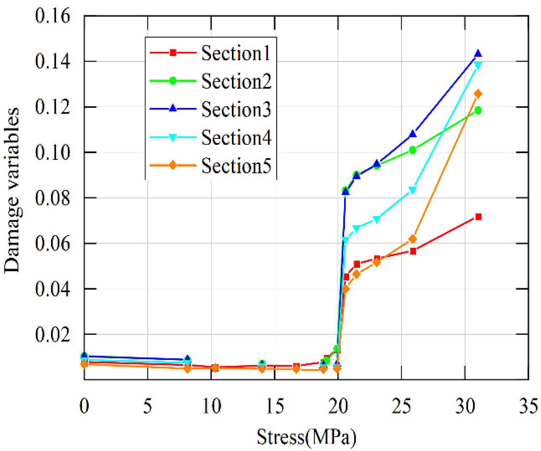
It can be seen from Figure 9 that there was basically no major damage on any section before σ = 20 MPa. There was also a small strengthening phase, which was caused by the CT-number-defining damage variable with density features, indicating that this phase accompanies the compaction process. After this stress, there was an almost vertical sharp rise, indicating a sharp expansion of the damaged area. The third segment was the largest, followed by the second and fourth segments, and the first and fifth segments were the smallest; the crack growth rate of each segment could be seen. This conclusion could be echoed in the image-analysis section.

6.1.2. Damage-Evolution Ratio

From Formula (3), the following damage-evolution ratio (Formula (4)) could be derived:

$$\stackrel{\ast }{D}=\frac{\mathrm{d}D}{\mathrm{d}\sigma }=\frac{D_{i+1}-D_i}{{\sigma }_{i+1}-{\sigma }_i}=\frac{(1-\frac{H_{rm(i+1)}}{H_{rm0}})-(1-\frac{H_{rmi}}{H_{rm0}})}{{\sigma }_{i+1}-{\sigma }_i}=\frac{H_{rmi}-H_{rm(i+1)}}{H_{rm0}({\sigma }_{i+1}-{\sigma }_i)}$$

(4)

We substituted the damage-variable values of each segment in each loading stage into Formula (4). The damage-evolution ratio that corresponded to each section at each loading stage could be calculated, and the relationship between the drawn stress and damage-evolution ratio is shown in Figure 10 below.

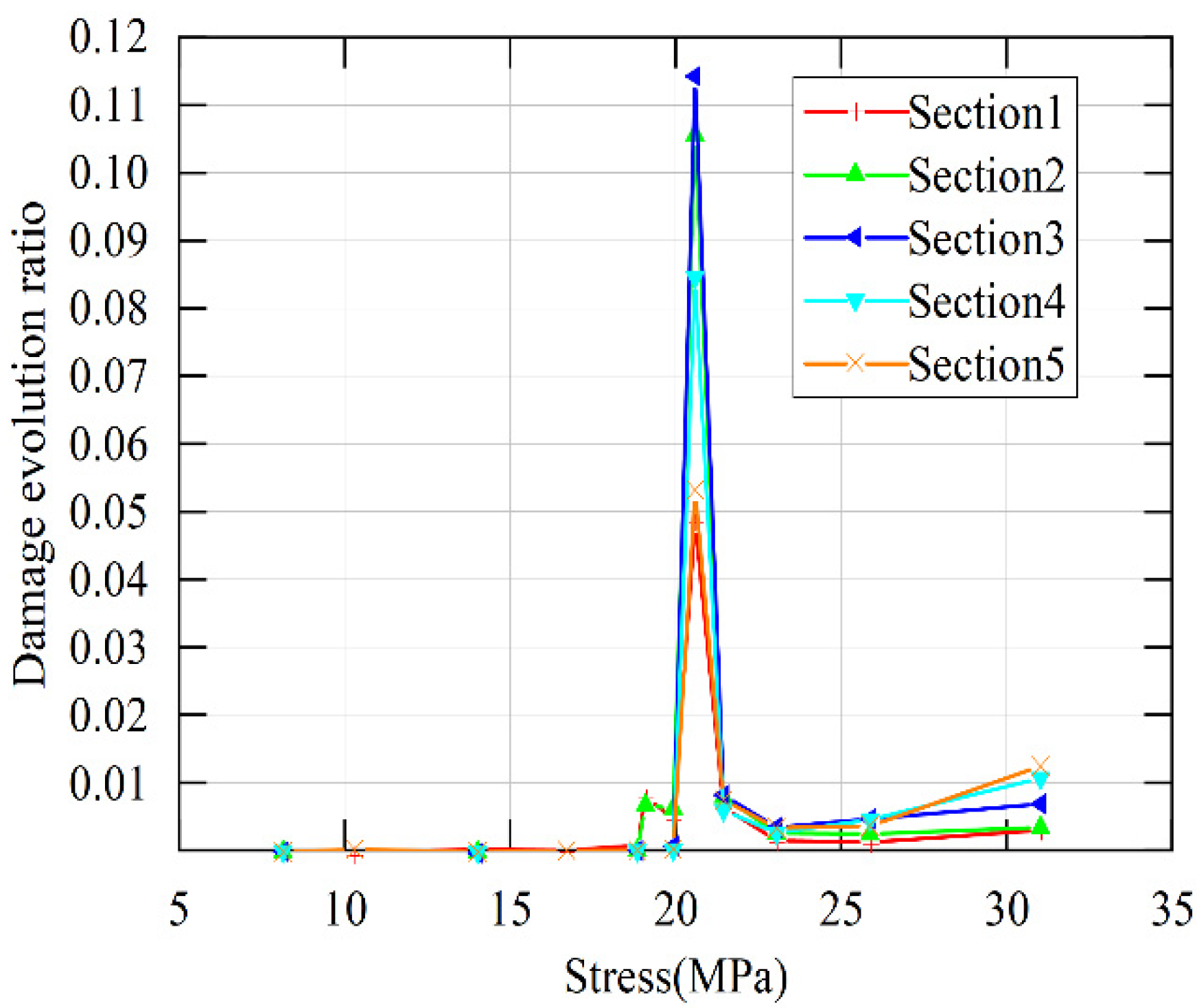
It can be seen from Figure 10 that when σ = 0.00 MPa~19.93 MPa, the damage-evolution ratio of each section had a negative process close to zero. This indicates a compression and strengthening phase, which is a process in which the amount of damage does not increase but decreases. There was a pulse peak at σ = 20.59 MPa. This showed that there was a damage-acceleration stage and the existence of a damage threshold. After that, the damage-evolution rate gradually decreased in the σ = 21.45 MPa~23.05 MPa stage, and it increased slightly in the σ = 23.05 MPa~25.88 MPa stage. The small increase or decrease in the damage-evolution ratio at this stage indicated that the crack was slowly expanding. Section 3 had the largest pulse amplitude, as confirmed by the sudden and rapid appearance of a through crack in the CT image. The second and fourth segments followed, the fifth-segment pulse peak was lower, and the first segment was the smallest. These phenomena, and the fractures in Segment 3 described in the previous mesoscopic analysis, emerged, and their propagation and penetration times were faster and more complete than in Segments 1 and 5. In contrast, Paragraphs 1 and 5 were slow in subsequent expansion and penetration. The appearance of cracks was consistent with the conclusion that the end-restraint condition was related to the uniaxial-compression condition, which justifies the conclusion. The pulse point of the damage-evolution ratio could be used as the reference point of the damage threshold, and the corresponding stress value was about 21.00 MPa, accounting for about 65.8% of the peak stress of 31.91 MPa.

6.1.3. Relationship between CT Number and Volume Strain

The deformation and failure process of rock is that a microcrack occurs, then accumulation and nucleation, and then gradual overlapping and connecting to form macrocracks. This fracture process was accompanied by volumetric compression and expansion, and this deformation was essentially due to the aforementioned damage. In the CT experiment, this damage could be reflected by the CT number, and the volume deformation of the rock could be regarded as the change in density.

Considering the experimental scan-layer thickness of 2 mm, the axial displacement at failure was only 1.2 mm, and the axial displacement averaged to the scan-layer thickness along the axis was only 0.02 mm. It could be considered that the same layer of material was scanned during the whole loading process, Hrm0 is the global average CT number in the initial state of the rock, and Hrmi is the global average CT number in a certain stress stage. Substitute this into the following relationship between the volume strain and CT number, as shown in Formula (5) [40,41]:

$${\epsilon }_v=\frac{H_{rm0}-H_{rmi}}{H_{rmi}+1000}$$

(5)

The volume strain was obtained by substituting the mean value of the CT number on the entire scanning plane of each section in each stress stage (including the initial scan), according to the statistics on the ROI, and substituting it into Formula (5). Draw the relationship curve between the stress and volume strain at each loading stage, as shown in Figure 11 below.

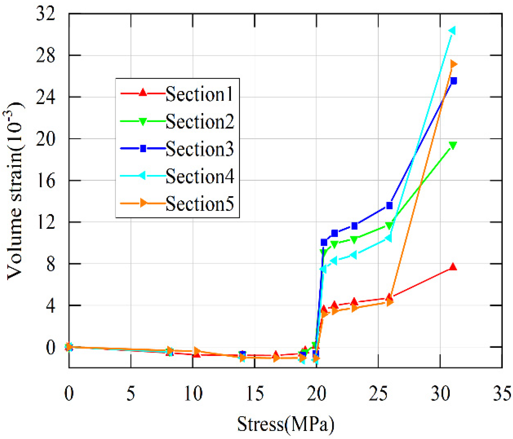
It can be seen from Figure 11 that the minimum volume strain of Section 1 was −0.00081 when σ = 16.71 MPa. The stage when the whole volume strain is negative is the volume-compression process, and the subsequent stage, when the volume strain is positive, is the volume-expansion process. At σ = 19.93 MPa, the volume strain became 0.00009, and then the volume expanded until it finally failed. The minimum volumetric strain of Section 3 at σ = 18.85 MPa was –0.00076. After that, the volume expansion changed to 0.01008 when σ = 20.59 MPa, and the transition range was larger and faster. This indicated that the crack propagated rapidly. When σ = 18.85 MPa, the volumetric strain of the fifth segment reached a minimum value of −0.001 09. The volume then expanded to 0.00314 at σ = 20.59 MPa.

The surge in the final phase indicated complete disruption, with a significant expansion in the transaction volume. The stage when the volumetric strain is negative is the compression process, and the curve was concave. The microcracks at this stage were mostly closed cracks. The subsequent positive phase was a process of overall expansion, manifested by the bottoming and rising on the curve. This is a process by which cracks open, connect, and develop into macroscopic cracks. As can be seen from the maximum volume shrinkage, Section 1 is −0.00081, Section 3 is −0.00076, and Section 5 is −0.00105. It can be seen that the volume reduction at both ends of the sample is greater than in the middle.

From the maximum value of the bulk strain of each section in the final failure stage, it could be seen that Section 3 was the largest, and Sections 5 and 1 were the smallest. The results showed that the process of volume expansion was opposite to the process of volume reduction; that is, the middle big end was small, which was related to the loading mode of uniaxial compression. The damage value corresponding to the stress stage with zero volumetric strain could be used as a reference point for the damage threshold, and the corresponding stress value was about 20.00 MPa, accounting for 62.7% of the stress peak value of 31.91 MPa. This stress could be used as the maximum design value. If this is greater than this stress, the sandstone may crack and fail.

6.2. Establishment of Damage-Evolution Equation

The damage-variable formula defined in this paper was replaced by the geometric and physical information (CT number) obtained from the partition description. The damage variable used here was the average value of the five-section damage variables at each stress stage. According to the relationship curve between the damage variable and the stress, the Boltzmann function of the form Polynomial (3) was used to fit the damage-evolution equation when σ = 0.00 MPa~21.45 MPa. Use Polynomial (4) to fit the damage-evolution equation at the stage of σ = 21.45 MPa~31.03 MPa.

$$D=\frac{A_1-A_2}{1+e^{\frac{\sigma -{\sigma }_0}{d\sigma }}}+A_2$$

(6)

$$D=B_2{\sigma }^2+B_1\sigma +B_0$$

(7)

In Formula (6), σ is the stress, and A₁, A₂, σ₀, and $d\sigma$ are experimental constants; in Formula (7), σ is the stress, and B₀, B₁, and B₂ are constants. The data used in the calculation and the fitting results are listed in

Table 4. List of fitting parameters and results of damage-evolution equation.

σ (MPa)	ε (10−3)	Section 1-D	Section 2-D	Section 3-D	Section 4-D	Section 5-D	D Mean	Fitting Parameters
0.00	0.00	0.0078	0.0105	0.0103	0.0087	0.0068	0.0088	A1 = 0.00688 A2 = 0.06871 σ0 = 20.32704 dσ = 0.11894
8.14	3.94	0.0065	0.0087	0.0088	0.0075	0.0049	0.0073
10.30	4.98	0.0055	0.0056	0.0054	0.0053	0.0052	0.0054
14.02	6.95	0.0062	0.0070	0.0064	0.0061	0.0048	0.0061
16.71	8.29	0.0061	0.0058	0.0054	0.0050	0.0047	0.0054
18.85	9.33	0.0077	0.0068	0.0063	0.0057	0.0047	0.0062
19.09	9.51	0.0110	0.0100	0.0096	0.0080	0.0064	0.0090
19.93	10.05	0.0135	0.0136	0.0070	0.0058	0.0049	0.0090
20.59	10.76	0.0455	0.0833	0.0824	0.0616	0.0400	0.0626
21.45	11.17	0.0510	0.0901	0.0894	0.0667	0.0464	0.0687	B0 = 0.2411 B1 = −0.0172 B2 = 0.0004
23.05	11.86	0.0533	0.0942	0.0948	0.0708	0.0517	0.0730
25.88	13.08	0.0567	0.1010	0.1079	0.0836	0.0619	0.0822

.

Substituting the constants obtained by fitting into the formula, the segmented expression of the damage-evolution equation is shown in the following formulas:

When σ = 0.00 MPa~21.45 Mpa:

$$D=\frac{-0.06183}{1+e^{\frac{\sigma -20.32704}{0.11894}}}+0.06871$$

(8)

When σ = 21.45 MPa~25.88 MPa:

$$D=0.0004{\sigma }^2-0.0172\sigma +0.2411$$

(9)

6.3. Partition-Damage Statistical Model

Based on the uniaxial-compression CT experiment on a certain sandstone, the rock samples were described in different areas (safety area, failure area, fracture area). On the basis of the obtained binary map of the evolution of the damaging zone and fracture zone, the address information of the damaging zone and fracture zone of each section at σ = 25.88 MPa was selected, and the CT information was used for statistical analysis. Then, the statistical-damage variable defined in this paper was calculated, and the mathematical expression of the damage-evolution equation was obtained by fitting. On this basis, the corresponding constitutive relationship between the safe area and damaged area could be obtained [42,43,44].

6.3.1. Constitutive Relation of the Safety Zone

According to the strain-coordination characteristics, the assumption of strain equivalence, and the principle of the effective stress of damage, because the deformation of the material safety zone in each stress stage is recoverable deformation, no irrecoverable damage is produced. Therefore, the linear elastic constitutive relationship in the form of Formula (10) is adopted:

$$\overline{\sigma }=E\epsilon$$

(10)

In the formula, the modulus is the elastic modulus in the nondestructive state, and its value is the modulus of the experimentally obtained elastic-stage material compressed to the densest state divided by 1−Di. Di is the damage-variable value of the stress stage corresponding to this state, and the calculated elastic modulus is 2.08 MPa.

6.3.2. Constitutive Relationship between the Damaging Zone and Fracture Zone

For the damaged zone and fractured zone of the material, because they are composed of CT units with different damage degrees, the damage constitutive relation is represented by a combination, as shown in the following formula:

$$\overline{\sigma }=(1-D)E\epsilon$$

(11)

When σ = 0.00 MPa~21.45 MPa:

$$\overline{\sigma }=[1-(0.06871-\frac{0.06183}{1+e^{\frac{\sigma -20.32704}{0.11894}}})]E\epsilon$$

(12)

When σ = 21.45 MPa~25.88 MPa:

$$\overline{\sigma }=\left[1-\left(0.005{\sigma }^2-0.02134\sigma +0.29792\right)\right]E\epsilon$$

(13)

The above formula is the constitutive relationship between the damaging zone and fracture zone at each loading stage. This formula, and the linear elastic constitutive relationship of the safe zone, constitute the constitutive relation of the material zone damage.

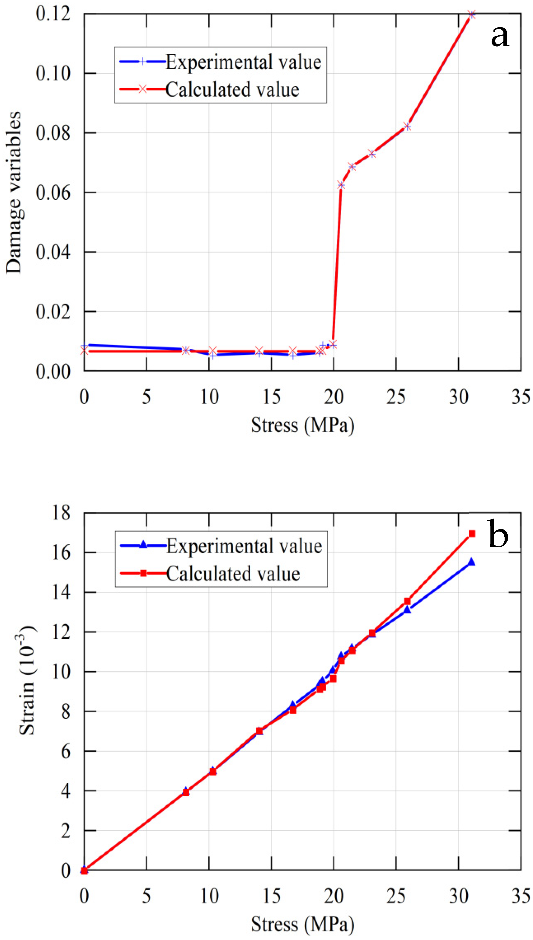
In order to test the rationality of the established damage-evolution equation and constitutive equation, 12 stress points were substituted into the above formula to compare the experimental value and theoretical-calculation value. The results are shown in Figure 12. The theoretical values in the figure refer to the results calculated by Formulas (12) and (13).

As can be seen from Figure 12, the calculated and experimental values of the damage variables fit well overall. Both the calculated and experimental values of the predamage stress were less than the threshold. Because the overall performance of the material had not changed much at this stage, the calculated values were in good agreement with the experimental values. In the final stage of damage, it could be seen that both errors were relatively large, and this was because the crack-penetration time was very fast at this stage, and it was suddenly too late to encrypt the scan. The data obtained by fitting were too small. In practice, other routine macroscopic experimental methods could be used to make up for this deficiency. The fusion of the two experimental methods could be carried out by means of stress–strain-process curves.

7. Conclusions

The following conclusions are based on a sandstone uniaxial-compression CT experimental study.

• In this paper, the idea of partition description was adopted: the data were classified and processed according to the specific situation, and the statistical error was eliminated to the maximum extent. Based on the CT experiment, the sandstone was described by partition theory. With the help of CT numbers, the research was advanced to the mesoscopic scale, the experimental results were discussed and analyzed, and the quantitative description of the CT experiment was realized;
• According to subarea description theory, the point sets that had different degrees of damage but were similar were divided into three areas: the safety zone, the damaging zone, and the fracture zone. This could reduce the interference of CT-number changes by uncertain factors, and it was conducive to data tracking and experimental data recording;
• The subarea thresholds H_e and H_d of the safety zone, the damaging zone, and the fracture zone were defined. By analyzing the CT images of five sections, it could be concluded that there is no monotonic trend in the minimum and maximum CT numbers. This showed that the appearance and stable expansion of cracks could be used as the threshold for dividing the damaging zone and fracture zone, and then ${\xi }_1$ = 50 and ${\xi }_2$ = 100 were selected;
• Based on the CT-test study on the damage-propagation characteristics of sandstone, using the CT number obtained by the partition-description theory, and on the basis of defined damage variables, a concise damage-evolution equation and damage statistical model of partition description were established. After calculation and comparison, it was found that the theoretical stress–strain curve was in good agreement with the measured curve.

References

- Uete, K.; Tani, K.; Kato, T. Computerized X-ray tomography analysis of three-dimensional fault geometries in basement-induced wrench faulting. Dev. Geotech. Eng. 2000, 84, 233–246. [Google Scholar]
- Tian, W.; Cheng, X.; Liu, Q.; Yu, C.; Gao, F.; Chi, Y. Meso-structure segmentation of concrete CT image based on mask and regional convolution neural network. Mater. Des. 2021, 208, 109919. [Google Scholar] [CrossRef]
- Song, M.; Wang, H.; Liu, H.; Liu, Z.; Zhang, C.; Li, J. Three-dimensional reconstruction of tight sandstone with CT scanning. Mater. Sci. Eng. 2019, 490, 052022. [Google Scholar] [CrossRef]
- Sun, X.; Li, X.; Zheng, B.; He, J.; Mao, T. Study on the progressive fracturing in soil and rock mixture under uniaxial compression conditions by CT scanning. Eng. Geol. 2020, 279, 105884. [Google Scholar] [CrossRef]
- Mcbeck, J.; Mair, K.; Renard, F. How Porosity Controls Macroscopic Failure via Propagating Fractures and Percolating Force Chains in Porous Granular Rocks. J. Geophys. Res. Solid Earth 2019, 124, 9920–9939. [Google Scholar] [CrossRef]
- Zaima, K.; Katayama, I. Evolution of Elastic Wave Velocities and Amplitudes during Triaxial Deformation of Aji Granite under Dry and Water-Saturated Conditions. J. Geophys. Res. Solid Earth 2018, 123, 9601–9614. [Google Scholar] [CrossRef]
- Zhang, L.; Dang, F.; Ding, W.; Zhu, L. Quantitative study of meso-damage process on concrete by CT technology and improved differential box counting method. Measurement 2020, 160, 107832. [Google Scholar] [CrossRef]
- Yang, S. Fracturing Mechanism of Compressed Hollow-Cylinder Sandstone Evaluated by X-ray Micro-CT Scanning. Rock Mech. Rock Eng. 2018, 51, 2033–2053. [Google Scholar] [CrossRef]
- Mihai, L.C.; Jefferson, A.D. A micromechanics based constitutive model for fibre reinforced cementitious composites. Int. J. Solids Struct. 2017, 110, 152–169. [Google Scholar] [CrossRef]
- Li, Y.; Li, L.; Bindiganavile, V. Constitutive Model of Uniaxial Compressive Behavior for Roller-Compacted Concrete Using Coal Bottom Ash Entirely as Fine Aggregate. Buildings 2021, 11, 191. [Google Scholar] [CrossRef]
- Soleymanzadeh, A.; Helalizadeh, A.; Jamialahmadi, M.; Soulgani, B.S. Development of a new model for prediction of cementation factor in tight gas sandstones based on electrical rock typing. J. Nat. Gas. Sci. Eng. 2021, 94, 104128. [Google Scholar] [CrossRef]
- Lester, A.M.; Kouretzis, G.P.; Pineda, J.A.; Cater, J.P. Finite element implementation of an isotach elastoplastic constitutive model for soft soils. Comput. Geotech. 2021, 136, 104248. [Google Scholar] [CrossRef]
- Khalaj, O.; Nejad, S.A.; Janda, T. Multi Elements Simulation of Biaxial Test with Two Different Soil Layers Using Hypoplastic Constitutive Model. IOP Conf. Ser. Mater. Sci. Eng. 2021, 1161, 012001. [Google Scholar] [CrossRef]
- Shrestha, K.C.; Aoki, T.; Miyamoto, M.; Wangmo, P.; Pema. In-Plane Shear Resistance between the Rammed Earth Blocks with Simple Interventions: Experimentation and Finite Element Study. Buildings 2020, 10, 57. [Google Scholar] [CrossRef]
- Nagy, Á.; Tóth, T.M.; Vásárhelyi, B.; Földes, T. Integrated core study of a fractured metamorphic HC-reservoir; Kiskunhalas-NE, Pannonian Basin. Acta Geod. Geophys. 2013, 48, 53–75. [Google Scholar] [CrossRef]
- Zhao, W.; Chen, W.; Yang, D.; Gao, H.; Xie, P. Analytical solution for seismic response of tunnels with composite linings in elastic ground subjected to Rayleigh waves. Soil Dyn. Earthq. Eng. 2020, 153, 107113. [Google Scholar] [CrossRef]
- Dong, C.; Lu, X.; Zhao, G.; Meng, X.; Li, Y.; Cheng, X. Experiment and Applications of Dynamic Constitutive Model of Tensile and Compression Damage of Sandstones. Adv. Mater. Sci. Eng. 2021, 2021, 2492742. [Google Scholar] [CrossRef]
- Wang, H.; Cheng, Y.; Lu, Z.; Zhu, Z.; Xue, Y.; Zhang, S. A Study on Constitutive Model of the Cohesive Soil Considering Soil-Structure Interactions. IOP Conf. Ser. Earth Environ. Sci. 2021, 719, 032033. [Google Scholar] [CrossRef]
- Hirai, T.; Shigeno, Y.; Takaji, K.; Iizuka, A. Study on Constitutive Model of Elastoplastic Behavior for Swelling Buffer Material. J. Appl. Mech. 2007, 9, 471–478. [Google Scholar] [CrossRef]
- Nikolinakou, M.A.; Whittle, A.J. Constitutive model of structural alteration and swelling behavior for old alluvium. Eng. Geol. 2021, 293, 106307. [Google Scholar] [CrossRef]
- Deng, F.; Chi, Y.; Xu, L.; Huang, L.; Hu, X. Constitutive behavior of hybrid fiber reinforced concrete subject to uniaxial cyclic tension: Experimental study and analytical modeling. Constr. Build. Mater. 2021, 295, 123650. [Google Scholar] [CrossRef]
- Guo, J.; Li, Y.; Zhai, R.; Yang, J. The Study on Plastic Flow Behavior and Constitutive model of GCr15 Steel in isothermal Compression. J. Phys. Conf. Ser. 2021, 1965, 012115. [Google Scholar] [CrossRef]
- Qin, C.; Zhao, W.; Zhong, K.; Chen, W. Prediction of longwall mining-induced stress in roof rock using LSTM neural network and transfer learning method. Energy Sci. Eng. 2021, 10, 458–471. [Google Scholar] [CrossRef]
- Zhao, W.; Qin, C.; Xiao, Z.; Chen, W. Characteristics and contributing factors of major coal bursts in longwall mines. Energy Sci. Eng. 2022, 10, 1314–1327. [Google Scholar] [CrossRef]
- Zhao, M.; Liu, G.; Liu, L.; Zhang, Y.; Shi, K.; Zhao, S. Bond of Ribbed Steel Bar in High-Performance Steel Fiber Reinforced Expanded-Shale Lightweight Concrete. Buildings 2021, 11, 582. [Google Scholar] [CrossRef]
- D’Aragona, M.G.; Polese, M.; Prota, A. Effect of Masonry Infill Constitutive Law on the Global Response of Infilled RC Buildings. Buildings 2021, 11, 57. [Google Scholar] [CrossRef]
- Talaromi, H.M.; Sakhaee, F. Evaluation and comparison of concrete constitutive models in numerical simulation of reinforced concrete slabs under blast load. Int. J. Prot. Struct. 2022, 13, 80–98. [Google Scholar] [CrossRef]
- Mihai, I.C.; Jefferson, A.D. Smoothed contact in a micromechanical model for cement bound materials. Comput. Struct. 2013, 118, 115–125. [Google Scholar] [CrossRef]
- Nishimura, S. A model for freeze-thaw-induced plastic volume changes in saturated clays. Soils Found. 2021, 61, 1054–1070. [Google Scholar] [CrossRef]
- Jefferson, A.D.; Mihai, I.C.; Tenchev, R.; Alnaas, W.F.; Cole, G.; Lyons, P. A plastic-damage-contact constitutive model for concrete with smoothed evolution functions. Comput. Struct. 2016, 169, 40–56. [Google Scholar] [CrossRef]
- Rossi, E.; Polder, R.; Copuroglu, O.; Nijland, T.; Šavija, B. The influence of defects at the steel/concrete interface for chloride-induced pitting corrosion of naturally-deteriorated 20-years-old specimens studied through X-ray Computed Tomography. Constr. Build. Mater. 2020, 235, 117474. [Google Scholar] [CrossRef]
- Otani, J.; Mukunoki, T.; Obara, Y. Characterization of failure in sand under triaxial compression using an industrial X-ray CT scanner. Int. J. Phys. Model. Geotech. 2002, 2, 15–22. [Google Scholar] [CrossRef]
- Kwon, J.; Lee, J.; Kim, H.S. Constitutive modeling and finite element analysis of metastable medium entropy alloy. Mater. Sci. Eng. A 2022, 840, 142915. [Google Scholar] [CrossRef]
- Yoshimitsu, N.; Kawakata, H.; Takahashi, N. Broadband P waves transmitting through fracturing Westerly granite before and after the peak stress under a triaxial compressive condition. Earth Planets Space 2009, 61, e21–e24. [Google Scholar] [CrossRef]
- Eghtesad, A.; Germaschewski, K.; Knezevic, M. Coupling of a multi-GPU accelerated elasto-visco-plastic fast Fourier transform constitutive model with the implicit finite element method. Comput. Mater. Sci. 2022, 208, 111348. [Google Scholar] [CrossRef]
- Yan, Y.; Zhang, L.; Luo, X.; Zhang, L.; Li, J. Process of porosity loss and predicted porosity loss in high effective stress sandstones with grain crushing and packing texture transformation. J. Pet. Sci. Eng. 2021, 207, 109092. [Google Scholar] [CrossRef]
- Farotti, E.; Mancini, E.; Lattanzi, A.; Utzeri, M.; Sasso, M. Effect of temperature and strain rate on the formation of shear bands in polymers under quasi-static and dynamic compressive loadings: Proposed constitutive model and numerical validation. Polymer 2022, 245, 124690. [Google Scholar] [CrossRef]
- Weihua, S.; Yongping, Z. Exploration and Research on Point Set Topology Teaching. Math. Learn. Res. 2014, 2014, 166–204. [Google Scholar]
- Xia, M.F.; Han, W.S.; Ke, F.J.; Bai, Y.L. Statistical meso-damage mechanics and damage evolution induced catastrophe. Prog. Mech. 1995, 25, 145–173. [Google Scholar]
- Wu, Y.Q.; Ding, W.H.; Cao, G.-Z. Observation of crack evolution process at uniaxial and triaxial CT scale in rock. J. Xi’an Univ. Technol. 2003, 19, 115–119. [Google Scholar]
- Ding, W.H.; Wu, Y.Q.; Pu, Y.B. Measurement of crack width in rock based on X-ray CT. J. Rock Mech. Eng. 2003, 22, 1421–1425. [Google Scholar]
- Wang, D.; Liu, E.; Zhang, D.; Yue, P.; Wang, P.; Kang, J.; Yu, Q. An elasto-plastic constitutive model for frozen soil subjected to cyclic loading. Cold Reg. Sci. Technol. 2021, 189, 103341. [Google Scholar] [CrossRef]
- Yamada, S.; Noda, T.; Nakano, M.; Asaoka, A. Combined-loading elastoplastic constitutive model for a unified description of the mechanical behavior of the soil skeleton. Comput. Geotech. 2022, 141, 104521. [Google Scholar] [CrossRef]
- Rocha, I.B.C.M.; Kerfriden, P.; van der Meer, F.P. Micromechanics-based surrogate models for the response of composites: A critical comparison between a classical mesoscale constitutive model, hyper-reduction and neural networks. Eur. J. Mech. A/Solids 2020, 82, 103995. [Google Scholar] [CrossRef]
Figure 1.
Laboratory CT-scan samples and equipment: (a) laboratory CT scanning machine; (b) laboratory CT-scan control computer; (c) laboratory CT-scan sample; (d) cross-sectional stratification of laboratory CT-scan specimens.
Figure 2.
CT-scan and stress–strain-relationship diagram.
Figure 3.
CT image of the first scan section: (a) σ = 0.00 MPa; (b) σ = 8.14 MPa; (c) σ = 10.30 MPa; (d) σ = 14.02 MPa; (e) σ = 16.71 MPa; (f) σ = 18.85 MPa; (g) σ = 19.09 MPa; (h) σ = 19.93 MPa; (i) σ = 20.5 MPa; (j) σ = 21.45 MPa; (k) σ = 23.05 MPa; (l) σ = 25.88 MPa.
Figure 4.
CT image of the third scan section: (a) σ = 0.00 MPa; (b) σ = 8.14 MPa; (c) σ = 10.30 MPa; (d) σ = 14.02 MPa; (e) σ = 16.71 MPa; (f) σ = 18.85 MPa; (g) σ = 19.09 MPa; (h) σ = 19.93 MPa; (i) σ = 20.59 MPa; (j) σ = 21.45 MPa; (k) σ = 23.05 MPa; (l) σ = 25.88 MPa.
Figure 5.
CT image of the fifth scan section: (a) σ = 0.00 MPa; (b) σ = 8.14 MPa; (c) σ = 10.30 MPa; (d) σ = 14.02 MPa; (e) σ = 16.71 MPa; (f) σ = 18.85 MPa; (g) σ = 19.09 MPa; (h) σ = 19.93 MPa; (i) σ = 20.59 MPa; (j) σ = 21.45 MPa; (k) σ = 23.05 MPa; (l) σ = 25.88 MPa.
Figure 6.
Statistical curve of CT number in ROI with loading process: (a) variation curve of CT number in ROI with stress; (b) variation curve of the variance in CT numbers in ROI with stress.
Figure 7.
The curves of the maximum CT numbers of the five cross-sections with the loading process: (a) the curves of the maximum values of CT number changing with stress in ROI; (b) the curves of the minimum values of CT number with stress in ROI.
Figure 8.
Calculation results of crack fractal dimension: (a) the yardstick logarithmic method; (b) the island method; (c) the box-counting method; (d) the sandbox method.
Figure 9.
Relationship between damage variables and stress on each scanning section.
Figure 10.
Curve of stress and damage-evolution ratio.
Figure 11.
Curve of stress and volume strain.
Figure 12.
Comparison of experimental values and formula-calculation results: (a) comparison chart of calculated and experimental values of damage variables; (b) comparison chart of calculated-strain value and experimental value.