Article

Retrieving Ocean Surface Winds and Waves from Augmented Dual-Polarization Sentinel-1 SAR Data Using Deep Convolutional Residual Networks

1
State Key Laboratory of Marine Environmental Science, College of Ocean and Earth Sciences, Xiamen University, Xiamen 361102, China
2
College of Earth, Ocean and Environment, University of Delaware, Newark, DE 19716, USA
3
Engineering Research Center of Ocean Remote Sensing Big Data, Fujian Province University, Xiamen 361005, China
4
Joint Institute for Coastal Research and Management (Joint-CRM), University of Delaware and Xiamen University, Newark, DE 19716, USA
*
Authors to whom correspondence should be addressed.
Atmosphere 2023, 14(8), 1272; https://doi.org/10.3390/atmos14081272
Submission received: 22 June 2023 / Revised: 3 August 2023 / Accepted: 8 August 2023 / Published: 11 August 2023
(This article belongs to the Special Issue Climate Change on Ocean Dynamics)

Abstract

:
Sea surface winds and waves are very important phenomena that exist in the air–sea boundary layer. With the advent of climate change, cascade effects are bringing more attention to these phenomena as warmer sea surface temperatures bring about stronger winds, thereby altering global wave conditions. Synthetic aperture radar (SAR) is a powerful sensor for high-resolution surface wind and wave observations and has accumulated large quantities of data. Furthermore, deep learning methods have been increasingly utilized in geoscience, especially the inversion of ocean information from SAR imagery. Here, we propose a method to invert various parameters of ocean surface winds and waves using Sentinel-1 SAR IW mode data. To ensure this method is more robust and scalable, we augmented the input data with dual-polarized SAR imagery, an incident angle, and a more constrained homogeneity test. This method adopts a deeper structure in order to retrieve more wind and wave parameters, and the use of residual networks can accelerate training convergence and improve regression accuracy. Using 1600 training samples filtered by a novel homogeneity test and with significant wave heights between 0 and 10 m, results from error parameters including the root mean square error (RMSE), scatter index (SI), and correlation coefficient (COR) show the great performance of this proposed method. The RMSE is 0.45 m, 0.76 s, and 1.90 m/s for the significant wave height, mean wave period, and wind speed, respectively. Furthermore, the temporal variation and spatial distribution of the estimates are consistent with China–France Oceanography Satellite (CFOSAT) observations, buoy measurements, WaveWatch3 regional model data, and ERA5 reanalysis data.

1. Introduction

Sea surface winds and ocean waves are critical phenomena in the air–sea boundary layer, affecting upper ocean dynamics and air–sea interactions. Therefore, large-scale continuous wind and wave observations are essential for wave climate and propagation research [1,2,3,4,5]. Buoy observations offer one possible method for attaining sea surface wind and ocean data. However, their typically sparse and nearshore locations mean they cannot provide enough of a spatial distribution to provide quality sea surface wind and wave observations. As a result, satellite observations have been an effective approach for the survey of dynamic ocean parameters. With its high-resolution two-dimensional imaging ability, Synthetic Aperture Radar (SAR) is able to capture more sea surface wind and wave information than a radar altimeter and radar scatterometer. Sentinel-1 SAR data are also free and can provide observations in nearly all weather conditions, both day and night.
SAR-based modulation transfer functions, including tilt modulation, hydrodynamic modulation, and nonlinear velocity bunching modulation, have traditionally been used to invert ocean waves via the ocean wave spectrum [6,7]. However, the nonlinear mapping relationship has become the basic theory of SAR wave inversion since it was proposed in 1991 [8]. Nonlinear modulation can cause the imaging process of ocean waves to be irreversible, but there are two ways to address this irreversibility. The first is to use wave model data as a constraint, meaning their representative methods are the “Max Planck Institute” algorithm [8,9] and the partition rescaling and shift algorithm (PARSA) [10]. The second way is to use parameterized winds as a constraint, with their representative methods being the semi-parametric retrieval algorithm [11] and the parameterized first-guess method [12].
Although a two-dimensional wave spectrum can reflect more information in ocean waves, the wave spectrum inversion requires prior information and numerous calculations because of the poly solution from the nonlinear imaging relationship. Therefore, empirical algorithms were proposed to retrieve integral ocean wave parameters such as significant wave height, wave period, and wave direction. For example, CWAVE extracts features from images and establishes an empirical relationship between the image feature parameters and the wave parameters using regression equations based on different satellites [13,14,15]. Other methods exploit the relationship between azimuth cutoff wavelength and wave parameters since the azimuth cutoff wavelength and some wave parameters are closely related through nonlinear velocity bunching [16,17,18]. More recently, a method based on dual-polarized SAR data has been proposed, improving the inversion performance by adding the input of VH-polarization data [19]. Simple machine learning approaches like support vector machines and backward propagation neural networks (BPNN), which are widely employed in regression processing, have also been applied to improve the inversion of wave parameters [15,20,21].
The parameters describing wind vectors include wind speed and wind direction. C-band SAR-derived wind speed estimation is based on empirical models such as the CMOD function for VV-polarized imagery (signal transmitted and received vertically), C-2PO, and C-3PO for cross-polarized imagery, respectively. CMOD geophysical model functions (GMFs) are generally used at low to moderate wind speeds due to signal saturation during high wind speeds, which include CMOD4, CMOD_IFR2, CMOD5, CMOD5.N, and CMOD7 [22,23,24,25,26]. At high wind speeds, the cross-polarized radar signals contain wave-breaking information, improving the high wind speed inversion results [27,28]. Since the wind speed inversion also needs regression processing, methods based on the BPNN have also been presented recently [29,30]. On the other hand, wind direction can be extracted in SAR imagery by the fast Fourier transform [31] and local gradient methods [32,33].
Deep learning (DL) methods have also improved over the past several years. One of the most common methods for classification and regression in DL is Convolutional Neural Networks (CNNs). They have strong performance capabilities in image processing and are suitable for feature extraction in SAR imagery. Moreover, CNN-based methods have been successfully applied to many SAR ocean-based remote sensing applications such as slick oil discrimination [34], ship detection [35], eddy detection [36], internal wave detection [37], significant wave height retrieval [38,39,40], sea ice classification [41], etc. Although many more CNN application examples appeared in classification or detection problems, the regression problem could be considered a classification problem with more categories.
Sentinel-1 SAR IW mode data distribute near the coast, which need a more precise match. The linear regression between wind or wave characteristics and the information from SAR imagery and spectra may then be less accurate. This occurs because the pattern of SAR spectra is very sensitive to wind and wave parameters nonlinearly, and the calculation of SAR features (i.e., azimuth cutoff wavelength) has strong uncertainties. Compared to previous linear methods, methods based on deep convolutional residual networks can extract large numbers of SAR image features, improving feature extraction during network training. Furthermore, as an important driver of ocean waves, wind is related to short ocean waves.
Thus, an adjusted deep Residual Network (ResNet)-based method for inverting wind and wave parameters using dual-polarized Sentinel-1 SAR IW mode data is proposed. This method is based on the analysis of SAR spectrum shape and magnitude for differing significant wave heights, wave directions, wavelengths, and wind speeds. The remainder of this manuscript is organized as follows: (1) Data and Methods are described in Section 2; (2) Results and Discussion are presented in Section 3; and (3) The Appendices specify the formulas and theories used in this study.

2. Data and Preprocessing

2.1. NDBC Buoy Data

Ground truth values of wind and wave parameters are essential to building the relationship between SAR imagery and target parameters when using a DL regression method. The CNN-based method is more reliable if high-precision wind and wave data are available. The standard meteorological historical data of 76 moored buoys from the National Data Buoy Center (NDBC) are used in this study, including wind speed and direction, significant wave height, mean wave period, dominated wave period, and mean wave direction. All the directions are degrees from true north, increasing clockwise. Anemometers aboard the buoys measure 5 m height wind speeds, which are converted to 10 m height wind speeds using the formula [42]:
u 10 = 8.7403 × u 5 ln ( 5 / 0.0016 )
The buoy data files contain year-long hourly data obtained from direct measurements, improving the regression’s reliability and verifying the inversion results. The distribution of NDBC buoys is shown in Figure 1, with all buoys located along the North American coastline.

2.2. ERA5 Reanalysis Data

Despite their availability, NDBC buoys are limited in the amount of high-seas state data they collect. The fifth-generation European Centre for Medium-Range Weather Forecasts (ECMWF) reanalysis (ERA5) hourly data for high sea state areas were retrieved from the Copernicus Data Store (CDS) to verify the inversion results. ERA5 estimates several parameters, including 10 m wind vectors, significant wave height, mean wave direction, mean wave period, and peak wave period. All reanalysis data, which have a 0.25° latitude-longitude grid and corresponding Sentinel-1 products, are downloaded to match the high sea state data.

2.3. Sentinel-1 SAR Data

As a part of the European Global Monitoring for Environment and Security satellite family, Sentinel-1 provides large-scale continuous free C-band SAR data and is a constellation consisting of two satellites: Sentinel-1A and Sentinel-1B [43]. According to the corresponding location and time of the NDBC buoys and ERA5 data, 2098 match-up Sentinel-1 Ground Range Detected (GRD) products were collected. All products are acquired by Interferometric Wide Swath (IW) and Stripmap (SM) modes and include VV and VH polarization SAR imageries. The Sentinel-1 HR (high-resolution) products with a 10 m spatial grid were selected for this study to unify the spatial grid of the input images. The resolution of IW mode SAR images is 20 × 22 m (range × azimuth), and the resolution of SM mode SAR images is 23 × 23 m. Incident angles for all images range from 32.9° to 43.1°.

2.4. Data Preprocessing

All Sentinel-1 imagery must be preprocessed before a relationship between SAR data and sea surface wind and waves can be established using CNNs. Therefore, three main preprocessing steps are performed and described below.
First, the SAR images are calibrated and converted to SAR spectra. All Sentinel-1 GRD products are displayed using digital numbers, which are unsuitable for wind and wave inversion, so calibration is used to convert these raw data to the NRCS values. Furthermore, the normalized radar cross-section (NRCS) is normally chosen as the raw input for the inversion process. However, waves have a higher correlation with the SAR-normalized self-correlation spectra, so the NRCS images are converted into SAR spectra. This process is further explained in Appendix A.
Secondly, spatial and temporal matching is performed for the SAR imagery and ground truthing data. To create a sample set for CNN training, only 224 × 224 sub-images of SAR data in the corresponding location, buoy data during the corresponding time, and corresponding ERA5 data are used. The central pixel of the SAR sub-image is nearest to the buoy’s position, and each sample has a temporal discrepancy of no more than one hour between the corresponding truth value and the SAR observation.
Finally, the input SAR image and SAR spectra are verified by a homogeneity test. The accuracy of wave inversion by the trained CNN is closely related to the correctness of the training samples. Thus, a homogeneity test and physical constraints are required for the training set. The modulation of SAR imagery over the ocean can be affected by many features, including the sea surface, islands, and ships. Buoys’ measurements can also differ from SAR observations, making CNN training deviate from the actual modulation relationship. Therefore, a homogeneity test performed on each SAR VV-polarization sub-image can help to avoid these problems by removing images with phenomena affecting inversion, like boundary layer rolls, atmospheric fronts, rain cells, sea ice, surface slicks, etc. More information about the homogeneity test can be found in Appendix B. The inhomogeneity parameter is calculated for each sub-image with a threshold of 1.05 to detect atmospheric fronts, slicks, and sea ice (Schulz-Stellenfleth and Lehner, 2004). Figure 2 shows example images of different inhomogeneity parameters (ξ). In general, features in SAR imagery appear more uniform when ξ is smaller than 1.05. The areas marked by red rectangles indicate irregularly high backscatter coefficients. Figure 2c shows inhomogeneity caused by atmospheric fronts that exhibit different scattering coefficients on both sides. In Figure 2d, the inhomogeneity is caused by land since it shows significantly high scattering coefficients.
In summary, the data preprocessing is conducted as follows: (1) Calibrate the SAR images to NRCS images and estimate the SAR self-correlation spectra; (2) According to the position and time of buoy observations, match the NRCS images and the SAR self-correlation spectra in the size of 224 × 224 to correspond to the size of the CNN input; and (3) Matching data will be tested by the inhomogeneity parameter with a threshold of 1.05.

3. SAR Imaging Feature and Proposed Method

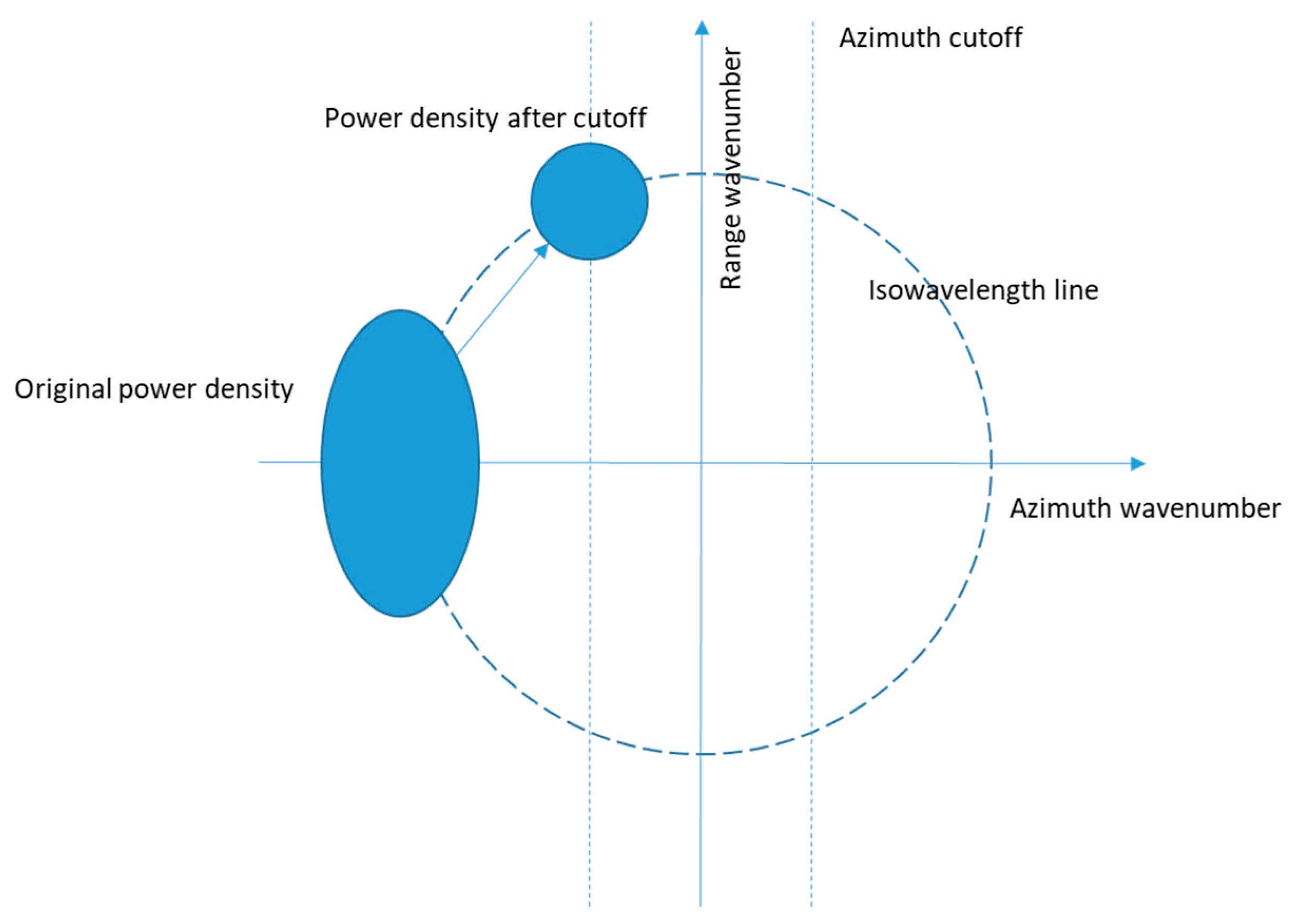
3.1. Relationship between Ocean Waves and SAR Images

SAR imagery and buoy measurements are different. Buoys measure ocean waves at a specific spatial point over a long time period, whereas SAR sensors measure ocean waves in a spatial area over a shorter period. Therefore, an understanding of the imaging theory is necessary for CNN design and validation.
Based on the fully nonlinear SAR wave imaging theory for VV-polarized data presented in Appendix C, the magnitude and pattern of SAR data are very sensitive to wave height, wave period, and wave direction. For a specific k y (x denotes the range, y denotes the azimuth), the Formula (A12) could be considered a linear term filtered by the exponential power of the slant range and velocity term. As k y increases, the linear term will increase while the exponential power will be reduced. As the exponential power term decreases, SAR spectra become visible only in a small range of azimuth wavenumbers. This relationship is not easily expressed as a linear function of wave parameters like significant wave height, peak wave period, and wave direction. However, the pattern and magnitude of SAR data are still related to the input wave spectra and the azimuth cutoff. The azimuth cutoff is mainly caused by the velocity bunching of SAR. Due to the Doppler shift, the scattering elements of the ocean waves heaving in the direction of SAR platform motion are shifted in the azimuth direction, which results in bunching at certain phases [44]. This procedure is called velocity bunching. As a result, the wave signal whose wavenumber is too high in the azimuth direction could not be displayed in the SAR spectra. Figure 3 shows the estimated SAR spectra and their magnitude of variation from ocean waves using Sentinel-1 parameters and the nonlinear imaging formula for different significant wave heights, wave periods, and wave directions.
JONSWAP wave spectra are used to simulate ocean wave spectra. The angular spread function affects the power density of the wave in the peak wavenumber, reflecting the angular dispersion of the ocean waves. This indicates that the magnitude of SAR spectra is lower when either the significant wave height is lower, the wave period is higher, or the wave direction is closer to the azimuth direction. The peak of SAR spectra is very close to the range direction and the peak wavenumber of JONSWAP wave spectra, which result from the azimuth cutoff and the nearest angular spread of JONSWAP. Moreover, according to Formula (A16), the azimuth cutoff is narrower when either the significant wave height is higher, the peak wave period is lower, or the wave direction is closer to the range direction.
Figure 3a–d shows how the significant wave heights significantly affect the azimuth cutoff and magnitude but have a smaller influence on the overall pattern. Figure 3e–h shows how wave direction significantly affects both the azimuth cutoff and magnitude as well as the change part of the SAR spectrum pattern. Figure 3e–h shows how the peak wavelength of a wave is closely related to the peak wavelength of SAR spectra. However, if the wavelength of the wave is too low, the SAR spectra will not express the wave linearly. This simple example could provide the basic relationship between wave parameters and SAR. However, the actual ocean waves are much more complex. Further analysis is essential.
In actual observation, there are many ocean waves in a single SAR spectrum. To discuss the SAR spectrum, which has ocean waves in different wavelengths and wave heights, the calculation is also necessary. In this case, we use the JONSWAP and angular spread functions to calculate different ocean waves for a single wave spectrum at the same time, which have different wave heights and wavelengths.
Figure 4 shows the different input wave spectra, including one or two wave systems. The significant wave heights, wave periods, and wave directions of the original wave and the added waves are shown in Table 1.
Overall, Figure 4 shows that a wave longer than the original wave system could significantly enhance the azimuth cutoff and reduce the magnitude of the calculated SAR spectra while leaving the peak wavenumber of the SAR spectra unchanged. Simultaneously, waves shorter than the original wave system can affect the pattern of the SAR spectra in the lower wavenumber but not the magnitude or azimuth cutoff of the SAR spectrum. This could be explained for a variety of reasons. First, although the pattern and magnitude of SAR spectra may be similar to those of the wave system without an exponential power term, the exponential power term distorts the pattern and magnitude of the wave expressed in SAR spectra, as the derivation in Appendix C shows. The exponential power term is determined by the Formula (A16). So, any power density in the wave system could increase the absolute value of the exponent in the exponential power term, thereby reducing the magnitude of the SAR spectra and making the azimuth cutoff narrower. Since the values of the velocity modulation function have a larger value at a high wavenumber, the influence of the short wave system is more significant.
Furthermore, the short wave of lower power density at a higher wavenumber will be affected by the stronger azimuth cutoff, which will further reduce the influence on the pattern of SAR. This essentially creates a positive feedback system. Conversely, long waves are less affected by azimuth cutoff, contributing little to it. So, it may affect the pattern of SAR spectra and even result in a higher power density in SAR spectra.
Then, we calculate SAR spectra for VV-polarization by using the buoy’s significant wave height, peak wave period, and peak wave direction. Since the JONSWAP wave spectra are an empirical calculation of ocean waves based on sea surface wind speed, they may not be exactly the same as the actual wave data. So, to establish the relationship between the SAR spectra and the actual wave parameters, a method based on a much stronger feature extractor, like deep learning, is necessary.
Figure 5 shows how the azimuth cutoff attenuates the original ocean wave power density signal. There is a distorted power density at the same wavelength due to the velocity of the original wave power. The shorter the wave, the more distortion there is, and the stronger the azimuth cutoff is.
Due to nonlinear effects like velocity bunching, SAR spectra cannot directly reflect ocean waves. However, ocean waves of different wave heights, wavelengths, and wave directions could be related to SAR spectra in different ways.
As Figure 3a–d shows, the higher the significant wave height is, the stronger the azimuth cutoff is. The nonlinear phenomenon will appear when the significant wave height is high enough. As Figure 3e–h shows, the closer to the azimuth direction the wave direction is, the more distorted the SAR spectrum indicates. But the closer to the range direction the wave direction is, the more complex the power density of the SAR spectrum indicates. Figure 3i–l shows that if the wavelength of an ocean wave is short enough, the nonlinear velocity bunching will make it more difficult for SAR spectra to reflect actual ocean waves. As a result, nonlinear phenomena appear, especially in ocean waves with high significant wave heights or low wave periods.
In conclusion, the ocean waves in very high and very low sea states have stronger nonlinear imaging effects, which are not suitable for regression using a traditional linear feature extractor. Therefore, the deep learning method is necessary. And to improve the results in a very high sea state, the VH images should also be used.

3.2. Relationship between Sea Surface Wind and SAR Images

As the main driving force of ocean waves, sea surface wind can also modulate the SAR NRCS images by changing sea surface roughness. The CMOD GMF provides a relationship between C-band SAR NRCS and wind parameters but was originally designed for wind retrieval from the scatterometer. However, the NRCS value can be expressed as a nonlinear function of the wind vector, radar incident angle, radar polarization, radar frequency, and some secondary parameters of the sea surface. Therefore, the GMF has the following format [22,23,24,25,26]:
σ 0 = b 0 ( V , θ ) [ 1 + b 1 ( V , θ ) cos φ + b 2 ( V , θ ) cos 2 φ ] p
where b 0 , b 1 , and b 2 are nonlinear functions of wind speed at a 10 m reference height ( V ) and incident angle ( θ ), p is a constant, and φ is the relative wind direction.
The algorithm for C-band VH-polarized (signal transmits in the vertical direction but is received in the horizontal direction) SAR data is presented to solve this issue due to signal saturation of VV-polarization data under high wind speed conditions. In addition to the methods based on GMF, the C3PO method is more simplistic:
σ 0 [ d B ] = ( 0.2983 V 29.4708 ) ( 1 + 0.07 θ 34.5 34.5 )
where σ 0 [ d B ] denotes the decibel value of NRCS, V denotes the wind speed at a 10 m reference height, and θ denotes the incident angle.
This method suggests that wind speed, wind direction, and radar incident angle can affect the NRCS of both VV-polarized and VH-polarized SAR data. The NRCS value for wind speed inversion is generally taken as the statistical value of a sub-image to suppress speckle noise. Additionally, wind speed inversion using a GMF needs wind direction as an input, so it is harder for SAR imagery to detect wind direction.
Traditionally, wind direction from SAR images is retrieved by the fast Fourier transform (FFT) and local gradients (LG) methods. They suppress the signals of short waves by filtering out signals with high wavenumbers and reducing spatial resolution (same as pooling in the CNN). This prevents the signals outside the azimuth cutoff area from affecting the results. However, local winds can drive short ocean waves, which correspond to low wave age and low phase speed in the ocean. This means that these methods are more suitable for retrieving the mean wind direction.
In conclusion, when wind direction and radar incident angle are known, the nonlinear GMF can extract wind speed from the SAR image. After removing low-wavelength signals, wind direction can be obtained from SAR spectra or local gradients. Since the DL method can capture more image features and regress the nonlinear relationship more effectively, CNNs can also be used to retrieve wind parameters.

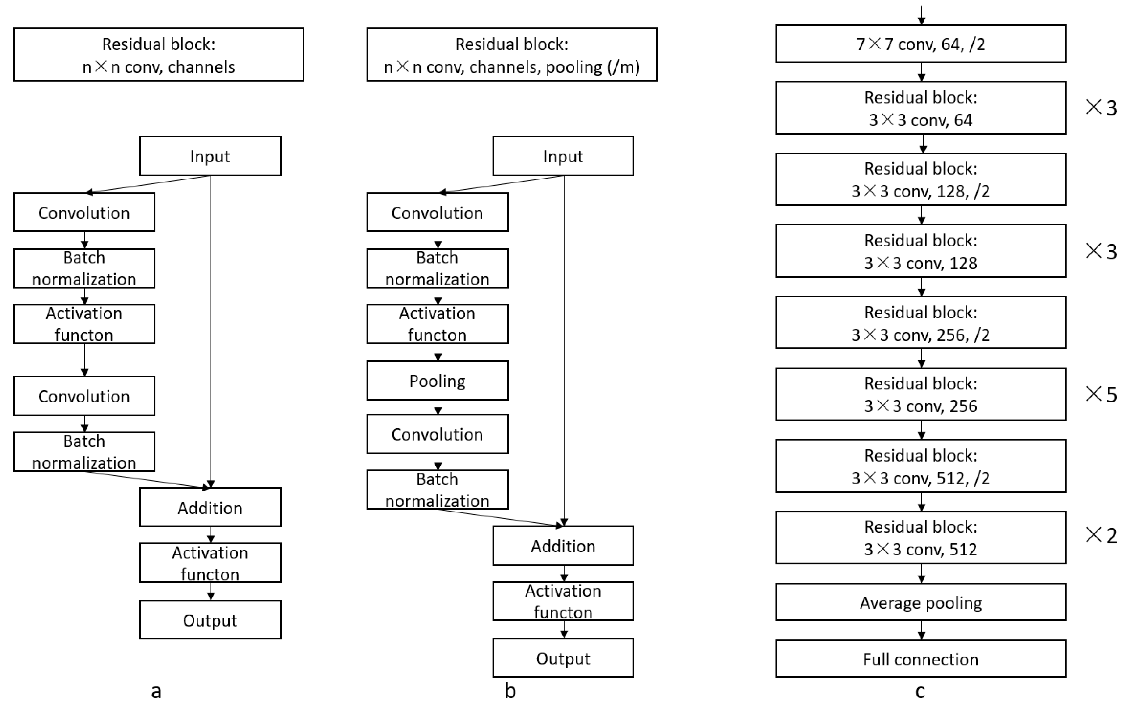
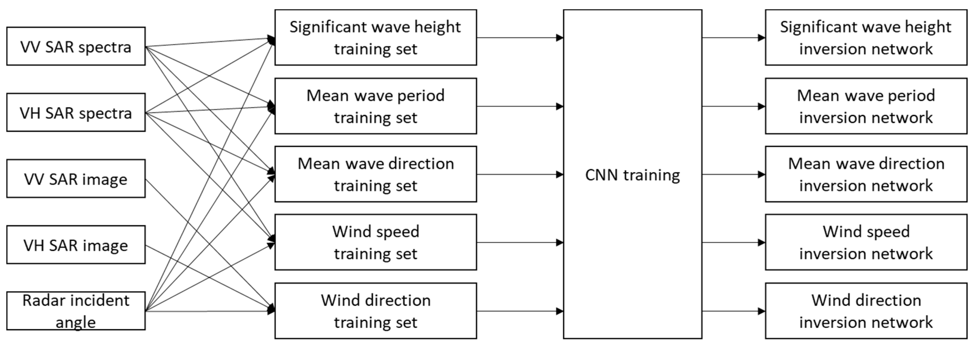
3.3. Inversion Method

The structure of CNNs has become deeper and more complex with the development of DL methods. However, adding layers may not always improve the regression efficiency but instead cause the network to converge on a higher training error. To solve these problems, residual networks (ResNet) are used [45]. Since the imaging mechanism of SAR for sea surface wind and waves is strongly nonlinear, ResNet can significantly improve the convergence speed and training effect. Therefore, ResNet is used to construct the inversion method in this study.
CNNs generally fit the desired feature maps directly using a succession of convolutional layers, pooling layers, batch normalization layers, and activation functions. In ResNet, a series of feedforward neural networks connect the feature maps, which skip one or more layers. For a single residual network, the stacked nonlinear layers fit the residuals of the input and output instead of directly fitting the original output. The residuals are easier to train than the original CNN output feature images. The CNNs without residual networks need much more training iteration, but the CNNs with residual networks need less iteration.
We take advantage of the residual network’s high regression efficiency in deep CNNs and use ResNet34 (34 hidden layers) to determine sea surface wind and wave inversion from SAR data. It consists of many residual blocks, whose structures are shown in Figure 6a. A layer of the convolutional network includes the stack of convolutional, batch normalization, and activation functions. The n denotes the size of convolutional kernels, and the channels denote the number of output feature maps. The residual operation is inserted before the activation function in the second layer of the convolutional network. If there is a pooling of layers after the first layer of the convolutional network in a residual block, the structure is converted to Figure 6b. The m denotes the size of the pooling. Figure 6c is the complete ResNet34 structure. First, the input images will go through a 7 × 7 convolutional network with a pooling of ×2. Second, they will go through 16 residual blocks of 3 × 3 convolution in sequence: 3 residual blocks with 64 channels, 1 residual block with 128 channels and 2 × 2 pooling, 3 residual blocks with 128 channels, 1 residual block with 256 channels and 2 × 2 pooling, 5 residual blocks with 256 channels, 1 residual block with 512 channels and 2 × 2 pooling, and 2 residual blocks with 512 channels. Finally, the target parameters could be derived after going through a 2 × 2 average pooling and a full connection layer.
The structure of ResNet34 is provided, but the details of some parameters, activation functions, and input and output need to be further defined. Since the magnitudes of wind and wave parameters are different, each parameter is retrieved by a specific neural network. According to the analysis of Section 3.1 and Section 3.2, wave parameters and wind direction are more closely related to the SAR spectra. In contrast, the wind speed is more closely related to the statistical value of the SAR NRCS image. Both the wind GMF and wave imaging functions vary with the incident angle, so the input image should include the incident angle. Moreover, the VH-polarized SAR image also contains wind and wave signals, so it should also be included in the input data.
As a result, the input image is defined as follows: For the inversion of significant wave height, mean wave period, mean wave direction, and wind direction, the VV-polarized SAR spectrum, VH-polarized SAR spectrum, and incident angle images are chosen as the input data. For the inversion of wind speed, the NRCS images for VV-polarized and VH-polarized and the incident angle images are chosen as the input data. For CNN training, the cost function is defined as the mean square error function. The activation function is defined as the Gaussian error linear unit function, which performs more effectively in nonlinear regression.
In summary, the training process is shown in Figure 7. The CNN is trained by the corresponding training set for each wind or wave parameter, and the CNN retrieves the wind and wave parameters after the training process.

4. Results

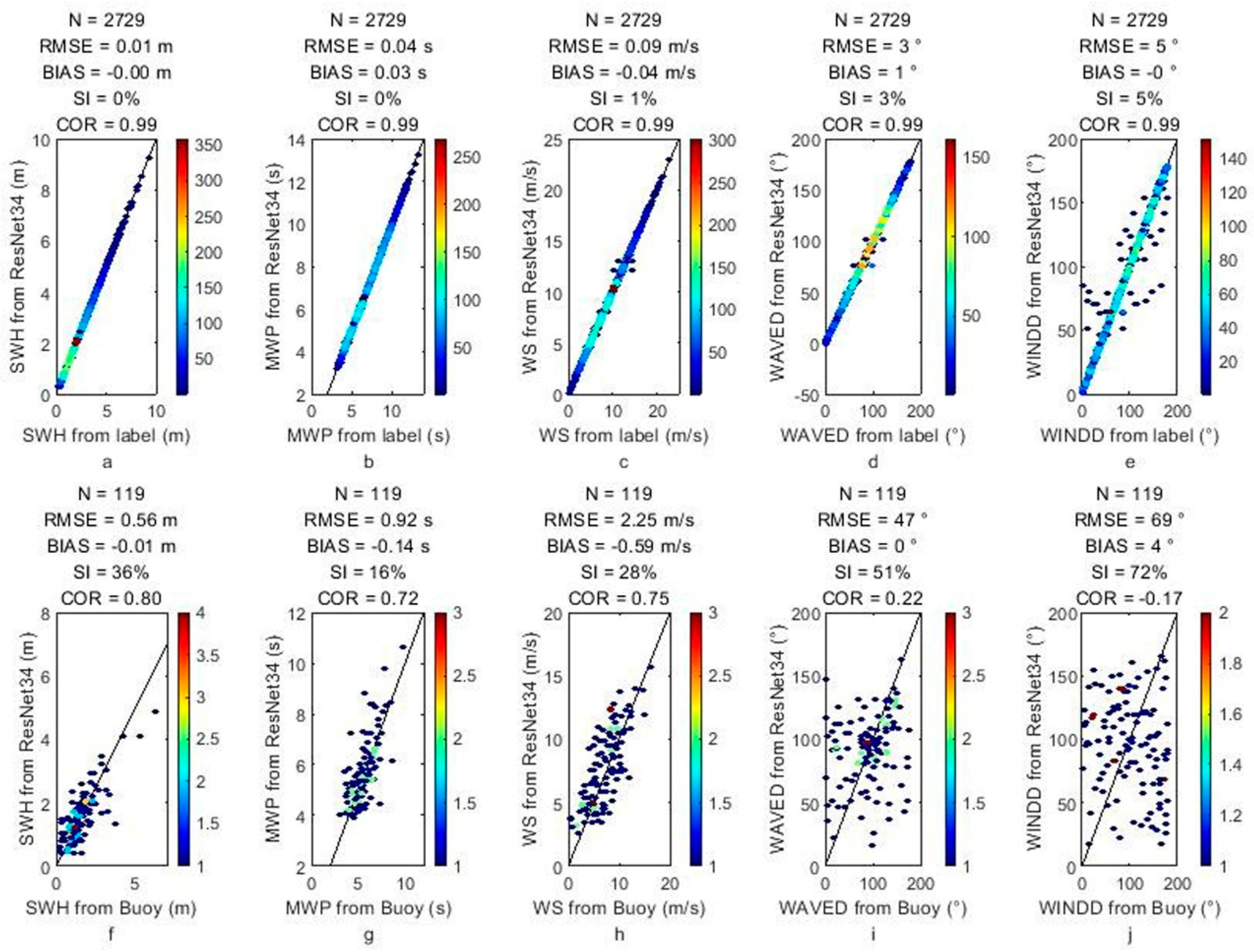
4.1. Training and Validation

Based on the analysis of sea surface wind and wave modulation and the powerful feature extraction capability of CNN, the training set of 2729 images is used for the significant wave height, mean wave period, mean wave direction, wind speed at a 10 m reference height, and wind direction. These parameters are trained using the adjusted ResNet34 network. Additionally, 119 samples matched with buoy data are used to verify the robustness and accuracy of the inversion method. The distribution of wind and wave parameters used in training and validation is presented in Figure 8. The top row denotes the distribution for the training wind and wave parameters, and the second row denotes the distribution for the validation wind and wave parameters. The validation set has the same distribution as the training set when the significant wave height is less than 7 m. The training set is trained by the adjusted ResNet34 with a single output. The batch size for training is 16, and the total training epoch is 1000.
Training and validation results are shown in Figure 9, where color denotes data density. The top-row scatter plots represent the training results of various wind and wave parameters, demonstrating the powerful regression ability of ResNet34. However, there are some outliers when training the wind direction data set. The bottom row of scatter plots shows the validation results for the inversion result out of the training set. Results indicate that significant wave height, mean wave period, and wind speed obtained from data other than the training set also have a good convergence trend. The validation results of error parameters for significant wave height, mean wave period, mean wave period, wind speed, and wind direction are shown in Table 2. However, the wind and wave direction results show large errors and a high scatter index in the validation set, meaning more samples for training might be necessary.

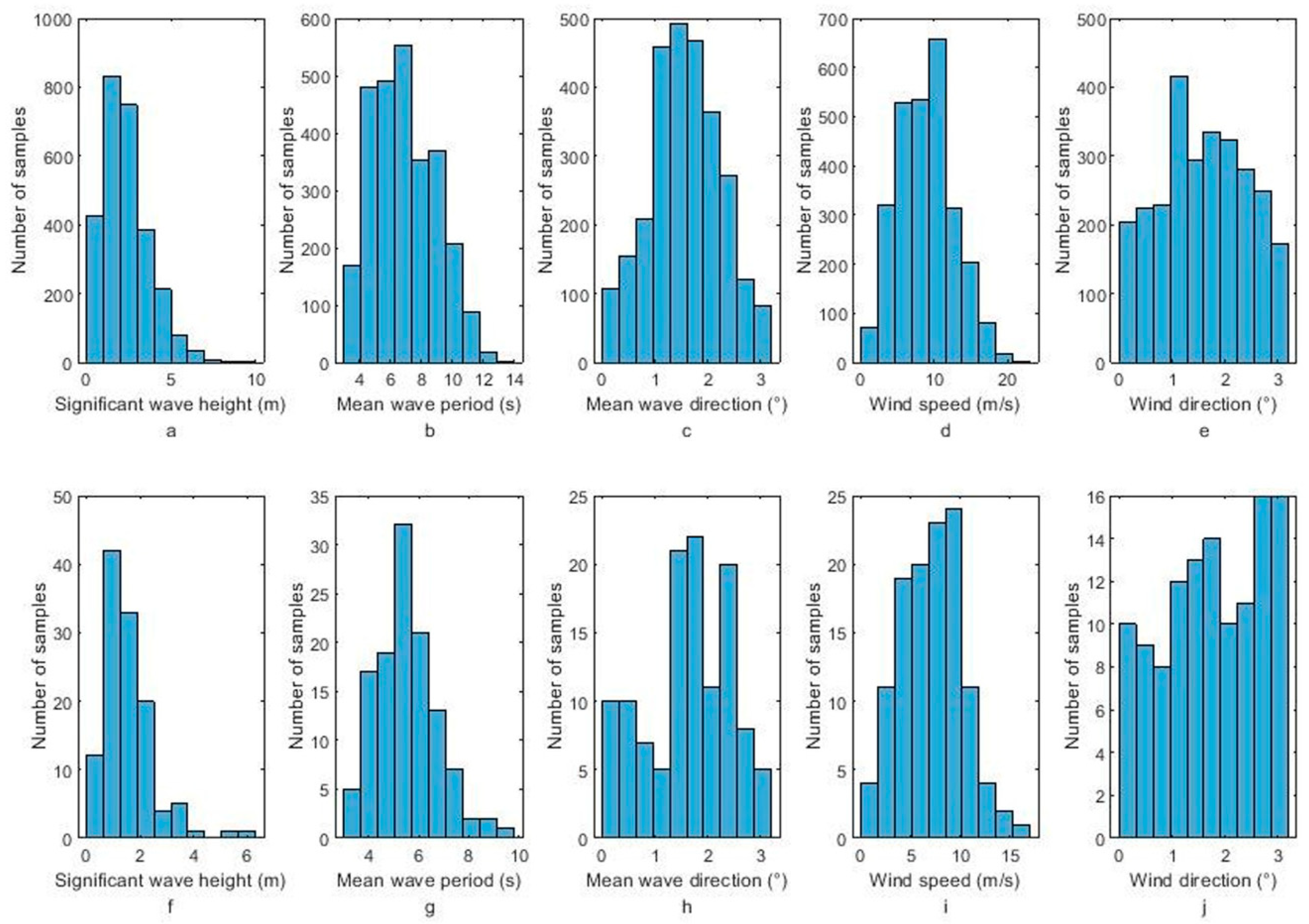
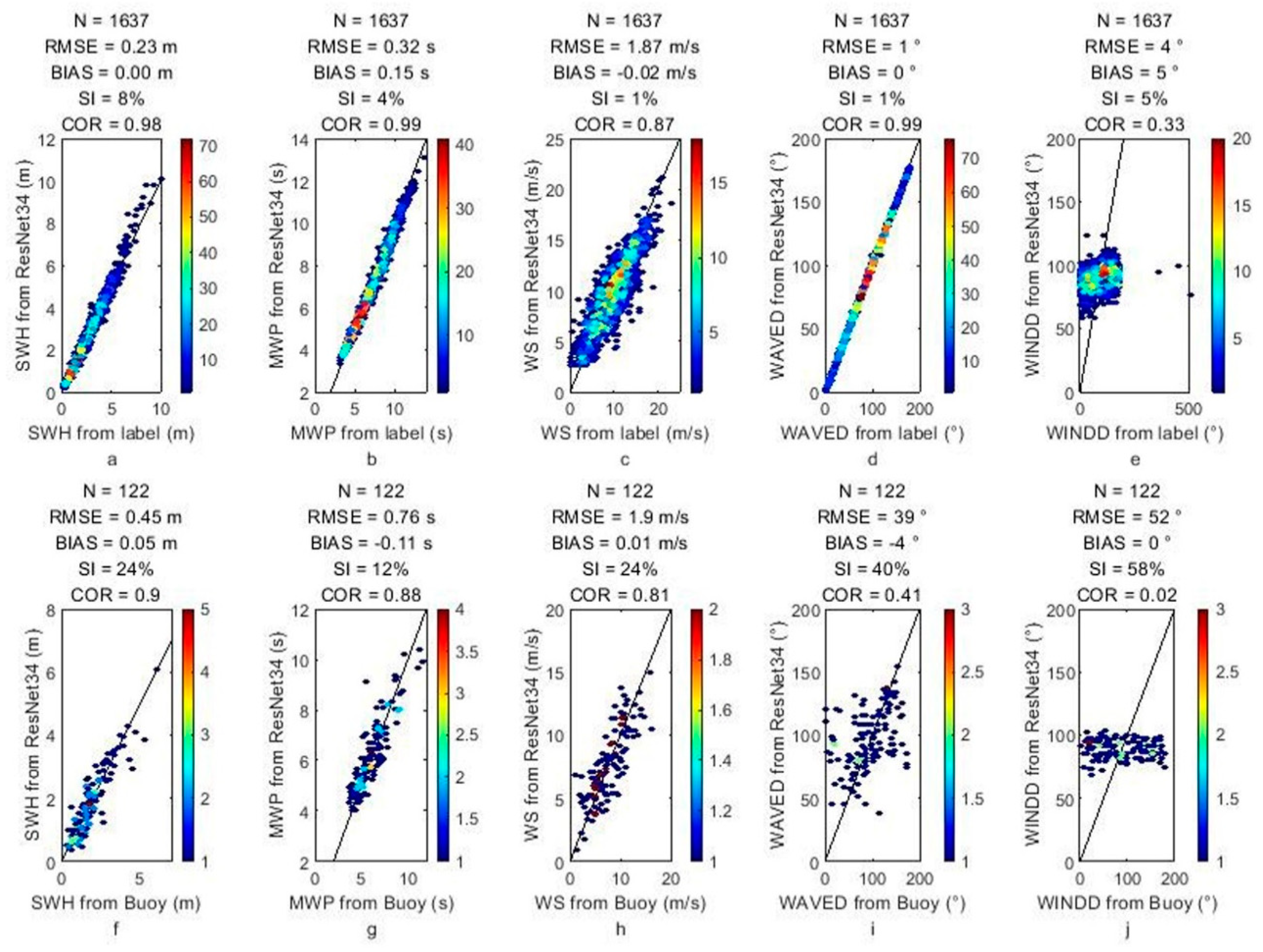
4.2. Constraint for a Training Set

For this data set, the retrieval of significant wave height, mean wave period, and wind speed is more suitable than the retrieval of wave direction and wind direction. The homogeneity test was able to remove the majority of inhomogeneous images. On closer inspection, inhomogeneous images have a central power density that is very high due to the inhomogeneous signals suppressing the signals of short wavelengths. Therefore, the weighted average wavenumber of the local maximum greater than 0.4 times the maximum power density is calculated to remove these leftover images. The samples whose weighted average wavenumbers of SAR spectra are less than 0.004 are further removed. The neural networks with the best test set results are selected for output.
The distributions of the filtered dataset are shown in Figure 10 and show that there is almost no change in the distributions compared to the original training set.
A total of 1600 samples are used to train the CNN for the inversion of wind and wave parameters, and 122 samples are used to verify the accuracy of the CNN. Figure 11 shows that the wind direction still cannot converge, but other parameters show better results in the validation data set. The validation results of error parameters for significant wave height, mean wave period, mean wave period, wind speed, and wind direction are shown in Table 3. The results of the mean wave direction show improvement and tend to converge, so it needs more training samples. Wind direction results did not converge in the training and validation sets. As most wind direction inversion methods use wind-induced streaks of larger wavelengths, the input images may need to have a larger spatial scale and be augmented by digital filters.
The results are also compared with former Sentinel-1 IW or SM mode SAR sea state inversion methods, especially in significant wave height, which is shown in Table 4. The inversion method using cutoff wavelength [17] validates the method using NDBC buoy data. The RMSE of the mean wave period is 1.86 s, and the RMSE of the significant wave height is 0.69 m. The CWAVE_S1-IW [46] method shows a 0.55 m RMSE of significant wave height compared with buoy data. The CWAVE_EX [47] method shows a 0.57 m RMSE of significant wave height and a 0.91 s RMSE of mean wave period compared with hindcast model data. The CWAVE_S1-IW and CWAVE_EX use rough spatial matching (>5 km) and interpolation in the temporal domain. It could affect the precision of IW mode data inversion results because IW mode data are distributed in the coastal area, whose sea states vary in the spatial domain. The inversion using shallow CNN [40] excludes data whose inhomogeneity parameters are higher than 0.5. Though it results in less available data, the available data have a more stable sea state. The RMSE of significant wave height is 0.32 m after using a lower homogeneity test threshold. The method proposed in this manuscript removes spectra whose density power is not concentrated at the coordinate center. The concentration of density power at the center means that the main signals of the spectra are at the longest wavelength, which is half the size of whole sub-images. It results from phenomena other than ocean waves, like fronts, oil spills, ships, etc. So, after removing those data, the input data have clear wave signals. The results show that the RMSE of the mean wave period is 0.76 s and the RMSE of the significant wave height is 0.45 m, which is better than the result of traditional methods. Although the shallow CNNs, which use lower inhomogeneity SAR data, have a lower RMSE of significant wave height, they may remove some data containing wave signals. In conclusion, the method proposed here not only archives multi-parameter inversion but also has better performance than traditional methods.

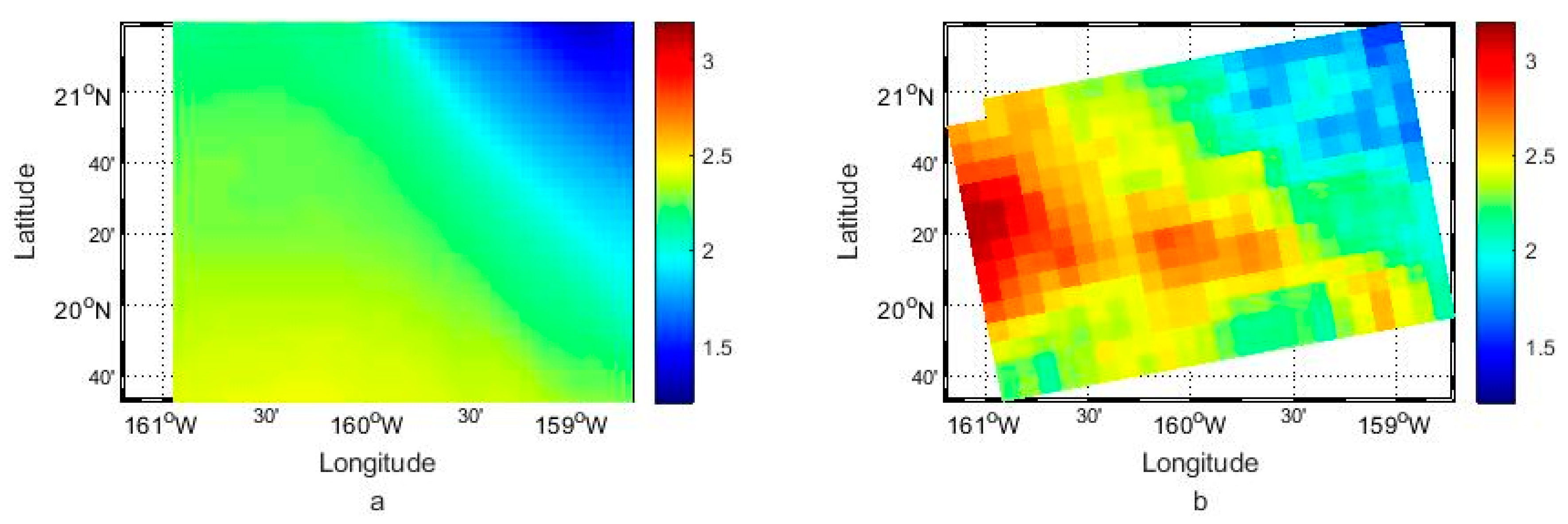
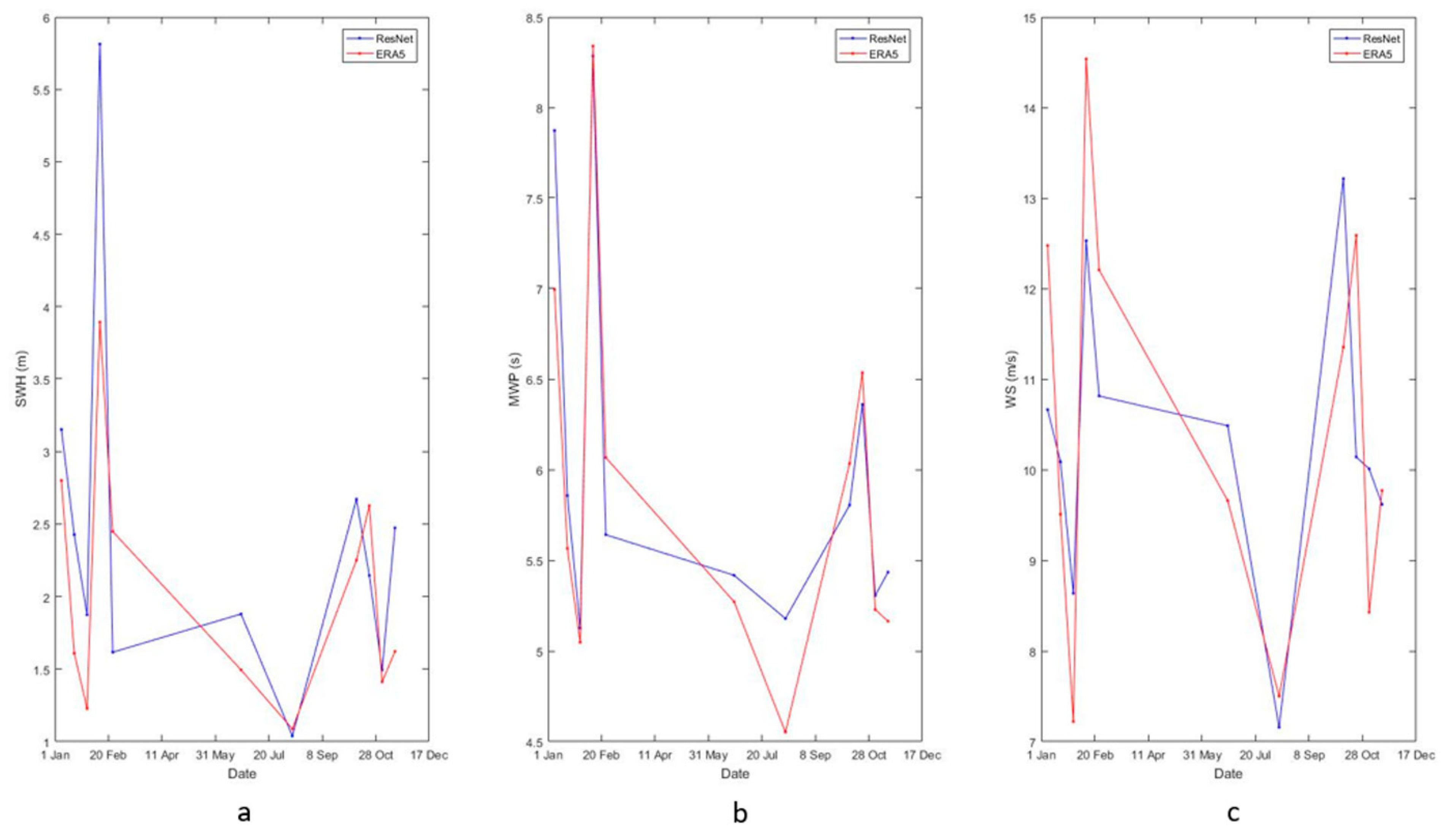
4.3. Further Validation by Some Examples

The comparison between buoy measurements and results from ResNet shows that ResNet is a very efficient tool for the inversion of significant wave height, mean wave period, and wind speed using only 1637 training samples. However, the results have not been verified for the spatial and temporal distribution, but some examples are provided in this section.
The first example compares WaveWatch3 Hawaii regional model data with significant wave height retrieved from SAR data by ResNet34. The grid size of WW3 data is 0.1°. To compare results in similar grids, here we use 1024 × 1024 sub-images, whose size is 10 km, to calculate the results. Figure 12 shows that the significant wave heights from model data indicate a distinct northeast-to-southwest gradient, which is also shown in the ResNet34 results. The significant wave heights from the CNN-based method could describe the spatial distribution. However, results from SAR data show a different pattern in certain areas. Some significant wave heights are higher than the model data, especially in the west. And it may be caused by the model data differing from the actual situation.
The second example compares the ERA5 reanalysis data temporal series located in the northern Taiwan Strait (120.46° E 25.69° N) and wave parameters retrieved from SAR data by ResNet34. The temporal variation in significant wave height, mean wave period, and wind speed retrieved from ResNet34 is generally consistent with the temporal trend of ERA5 data (Figure 13).
Model and reanalysis data are not as reliable as measured data. Therefore, the CFOSAT data are also used for validation, which contains wave directional spectra from SWIM (a sensor that measures waves), wind speed from a scatterometer, and typical wave parameters. The wave spectra from CFOSAT data also estimate the mean wave period. To compare the spatial distribution in depth, four SAR images observed on 20 December 2020 on the west coast of North America are used. The third sample is the spatial comparison between along-track CFOSAT data and the ResNet34 inversion results, shown in Figure 14. The SAR images are divided into sub-images of 1024 × 1024, and the parameters are retrieved from the center 224 × 224 pixels of the sub-images. The significant wave height, mean wave period, and wind speed show the same spatial variation from CFOSAT and ResNet34 along the track of CFOSAT. And the distribution also satisfies the law of ocean wave growth, which states that as waves mature, their wave height and wave period increase while the wind speed remains constant. Although the regions of 44–45° N and 126–128° W have lower wind speeds, the waves are more mature. Therefore, it also expresses high and significant wave heights in this region. However, there is a temporal interval of 1–2 h here. So, the results of local wind have more differences between CFOSAT and SAR.
The Sentinel-1 IW mode images covering the NDBC 46050 buoy located at 124.546° W 44.669° N on the west coast of North America are also in the same region as the northeast SAR image in the former sample to verify the temporal variation using the buoy measurement data. Only six images pass the homogeneity test, and the temporal variation in wave parameters retrieved by ResNet34 is nearly the same as that observed by the buoy (Figure 15a,b). As Figure 15c shows, the wind speed retrieved by ResNet34 seems to have a large error on 20 December 2020. Both the ResNet34 results and buoy observations show an initial decrease followed by an increase before 20 December 2020. Since the homogeneity test may have little effect on wind speed inversion, the images that have not passed the homogeneity test are also used for validation. Results show that the variation in wind speed between ResNet34 and the buoy over time is almost the same (Figure 15d).

5. Conclusions and Discussion

Since certain wave information may be reflected in SAR spectra, and the NRCS is related to the wind vector, ResNet34 shows a powerful regression capability in regressing SAR spectra or SAR images to winds and wave parameters. ResNet34 is trained by 1600 samples to retrieve the significant wave height, mean wave period, and wind speed and is verified by other observational data. The result of significant wave height shows a bias of 0.05 m, an RMSE of 0.45 m, a SI of 24%, and a COR of 0.90. The result of the mean wave period shows a bias of −0.10 s, an RMSE of 0.76 s, a SI of 12%, and a COR coefficient of 0.88. The wind speed result shows a bias of −0.01 m/s, an RMSE of 1.90 m/s, a SI of 24%, and a COR of 0.81. Moreover, the inversion results can also describe the spatial and temporal variation, as verified by measured data, model data, and reanalysis data. Results also conform to the ocean wave growth theory.
Using a lower homogeneity test threshold, the former CNN-based technique for significant wave height inversion appears to perform well. However, SAR data containing valid information can be removed, but the expansion of the application requires the input of more training samples. The method in this study retrieves more wind and wave parameters, which is more robust and scalable.
Although this method could retrieve significant wave height, mean wave period, and wind speed from Sentinel-1 SAR dual-polarized data with 10 m pixel spacing, it can still be further improved. First, the inversion of mean wind direction and mean wave direction is not feasible using this process. The sub-image size in this article is too small to obtain wind streak information caused by Langmuir circulation. And, since a single radar measurement could not solve the wind direction inversion, the sub-aperture of the SAR image should be used in the wind direction inversion. Furthermore, the cross-polarized images have scalloping effects, which should also be further considered, though CNN may learn about these effects on its own.
Second, the deeper structure of CNNs requires longer training times and more GPU memory. The structure needs to be simplified, and the structure of the residual networks needs to be preserved to enhance computing efficiency.
Third, since the incident angle of the SAR data used for training ranges only from 32.9° to 43.1°, some of the imagery may not accurately invert these parameters while the incident angles are outside of this range.
Furthermore, different satellites have different flight speeds and orbital altitudes, which makes this method hard to extend to other satellites only trained by Sentinel-1 data. An attempt was made on Hisea-1, the first C-band SAR small satellite for ocean remote sensing [48]. Hisea-1 is limited to VV-polarized data, so ResNet34 for only inputs of VV-polarization data is trained by Sentinel-1 data. After unifying the azimuth cutoff ( β ), parameters are retrieved from Hisea-1 data. Only a sample whose incident angle is from 32.9° to 43.1° fits the buoy measurement, which is not enough to prove that this method could be extended within a certain range of incidence angles. Therefore, collecting more matching samples of the Hisea-1 data and the measured data is necessary. It could also be used to train the new CNN for Hisea-1 inversion and verify this method’s scalability.
In conclusion, the inversion method based on ResNet34 can more precisely retrieve significant wave height, mean wave period, and wind speed. Trained with 1600 samples, this method can be extended to other regions and provide temporal variation and spatial distribution for these parameters. Using transfer learning, this method can be further improved with the accumulation of data in different situations. The pixel spacing of the parameters retrieved by this method reaches 2.24 km, corresponding to 224 × 224 sub-images. However, the results for a very high sea state should be further verified.

Author Contributions

Conceptualization, S.X.; Methodology, S.X.; Validation, S.X.; Data curation, S.X. and H.S.; Writing—original draft, S.X.; Writing—review & editing, L.M., X.G., D.E. and X.-H.Y. All authors have read and agreed to the published version of the manuscript.

Funding

This work is supported by the National Key R & D Program of China (2019YFA0606702), the National Natural Science Foundation of China (Grant Numbers: 91858202, 41630963, and 41776003), and Industry–University Cooperation and Collaborative Education Projects (202102245034). Xiao-Hai Yan has been supported by the NSF (IIS-2123264) and NASA (80NSSC20M0220). The authors would also like to thank Fujian Haisi Digital Technology Co., Ltd. and Fujian Tendering Purchasing Group Co., Ltd. for supporting this research.

Data Availability Statement

No new data were created or analyzed in this study. Data sharing is not applicable to this article.

Conflicts of Interest

The authors declare no conflict of interest.

Appendix A. Calibration and SAR

The digital number of SAR images read from geotiff files can be converted to the NRCS by calibration parameters read from the extensible annotation markup language (xml) file in the products. The look-up tables (LUT) of ‘sigmaNought’ and ‘noiseLut’ are used in the calibration. The complete calibration parameter matrix can be obtained by two-dimensional linear interpolation of the LUT. For each pixel, the NRCS value is calculated by the formula below:
NRCS = D N 2 n o i s e s i g m a 2
where noise and sigma are the values of the interpolated ‘noiseLut’ and ‘sigmaNought’ for each pixel, and DN is the original digital number of SAR images for each pixel. NRCS is the calibrated value for each pixel.
After calibration, SAR images will be cropped to a size of 224 × 224, corresponding to the buoy position. Since sea surface waves are more closely related to SAR spectra, the NRCS images should be further processed. And SAR is not directly obtained by the 2D-FFT of the NRCS image. The normalized image is defined as I :
I = N R C S N R C S N R C S
represents the mean of the matrix inside the angle brackets, and the NRCS represents the NRCS values in the sub-image in size N = 224 . Then, the 2D-FFT is applied to the normalized image:
F I = f f t 2 D ( I )
The SAR is the power density I , which is also the self-correlation I in a mathematical sense:
P = | F I | 2
To make the integral in the wavenumber domain equal to the integral of the image in the spatial domain, the SAR spectra are normalized by the following formula:
P = P P d k x d k y
d k x and d k y are the wavenumber intervals in the range direction and azimuth direction, respectively, which could be calculated by the range pixel spacing d x and azimuth pixel spacing d y :
d k x = 2 π N d x d k y = 2 π N d y
Gaussian filtering is performed on the SAR spectra, whose standard deviation and window size are 1.6 and 5, to make the SAR spectra appear smoother.

Appendix B. Homogeneity Test

The homogeneity test aims to check whether the image has stable features at various spatial positions. Firstly, the 224 × 224 sub-image is further cropped to a size of 56 × 56. The homogeneity of the 224 × 224 images can be judged by the statistics of the spectral features of these 16 resulting sub-images.
As the distribution of power density values satisfies a negative exponential distribution for each specific wavenumber pixel in the spectral domain, the square mean and the variance of the power density for each wavenumber should be nearly equal. So, the inhomogeneity parameter can be denoted as the weighted mean of variance divided by the mean square. The expression is described as follows:
ξ H = k var i [ P i ( k ) ] / m e a n i [ P i ( k ) ] k m e a n i [ P i ( k ) ] ,
where i denotes the serial number of the 56 × 56 sub-images, k is the wavenumber, var i [ P i ( k ) ] is the variance of power density in different sub-images for the specific wavenumber, and m e a n i [ P i ( k ) ] is the average of the power density in different sub-images for the specific wavenumber.

Appendix C. Nonlinear SAR Wave Imaging Theory

In general, there are four main modulations for SAR wave imaging: tilt modulation, hydrodynamic modulation, range modulation, and velocity modulation in the slant range direction, which can be expressed, respectively [8,9]:
T k h y d r = 4.5 ω k x 2 ( ω i μ ) | k | ( ω 2 + μ 2 )
T k r a n g e = i k x cot θ
T k v = ω ( i cos θ + k x | k | sin θ )
T k R = T k t i l t + T k h y d r + T k r a n g e
where k x denotes the range wavenumber, k y denotes the azimuth wavenumber, θ is the incident angle, ω is the circular frequency of the wave, and μ is the attenuation coefficient, which is usually taken as 0.5. The first three modulations are the real aperture radar (RAR) modulations. The last modulation represents the relative velocity in the direction of the slant range from the radar to the target. After some derivation, the nonlinear imaging formula could be obtained. The power density ( P S ( k ) ) can be denoted as:
P S ( k ) = ( 2 π ) 2 d r exp ( i k r ) exp [ k y 2 β 2 f v ( r ) k y 2 β 2 f v ( 0 ) ] { f R ( r ) + 1 + i k y β [ f R v ( r ) f R v ( r ) ] + k y 2 β 2 [ f R v ( r ) f R v ( 0 ) ] [ f R v ( r ) f R v ( 0 ) ] }
where β = R / V , R is the slant range between SAR and target, V is the flight velocity, f R ( r ) , f v ( r ) , and f R v ( r ) denotes the correlation of the RAR part and slant range velocity part:
f R ( r ) = < I R ( x + r ) I R ( r ) > = 1 2 { F ( k ) | T k R | 2 + c . c . } e i k r d k
f v ( r ) = < v ( x + r ) v ( r ) > = 1 2 { F ( k ) | T k v | 2 + c . c . } e i k r d k
f R v ( r ) = < I R ( x + r ) v ( r ) > = 1 2 { F ( k ) T k R ( T k v ) * + F ( k ) ( T k R ) * ( T k v ) } e i k r d k
The Formula (A12) for P S ( k ) is similar to 2D-FFT but k y is present in the Fourier operator. It is not a Fourier transform unless k y is a constant or a function in the spatial domain. To use the FFT to speed up the calculation efficiency of this integral formula, this formula could be understood in another way: k y is only different on the azimuth axis. So, for each specific azimuth wavenumber, the FFT can be calculated. Only the FFT results for this azimuth wavenumber are selected as part of the final result. The amount of calculation is determined by the side of the azimuth direction (224 in this study).
The nonlinearity of SAR imaging mainly results from the exponential power terms: exp [ k y 2 β 2 f v ( r ) k y 2 β 2 f v ( 0 ) ] . As Formulas (A14) and (A10) show,
f v ( 0 ) = k ω 2 ( cos 2 θ + sin 2 φ sin 2 θ ) F ( k ) d k
where φ  represents the wave direction (0 denotes the positive azimuth wave number). Assuming that the wave is a JONSWAP spectrum for infinite water depth, for a specific significant wave height and a specific wave period, the power density of a wave in peak wavenumber would vary with φ  according to the angular spread function. The wave and the angular spread function used in SAR simulation in this study are defined as follows (Sun and Kawamura, 2009):
S ( ω ) = α g 2 ω 5 exp [ 1.25 ( ω 0 ω ) 4 ] γ exp [ ( ω ω 0 ) 2 2 σ 2 ω 0 2 ]
G ( ω , φ ) = 0.5 b   sech 2 b ( φ φ m )
where ω 2 = g k , k = k x 2 + k y 2 , and φ = arctan ( k x k y ) ( k y > 0). α depends on the significant wave height. And b denotes how the power density of the wave varies with φ , which is defined as:
b = { 2.61 ( ω ω 0 ) 1.3 , 0.56 < ω ω 0 < 0.95 2.28 ( ω ω 0 ) 1.3 , 0.96 < ω ω 0 < 1.6 1.24 , else
The F ( k ) is expressed as:
F ( k , φ ) = S ( ω ) G ( ω , θ )
And the significant wave height is:
s w h = 4 k F ( k ) d k

References

  1. Camus, P.; Losada, I.J.; Izaguirre, C.; Espejo, A.; Menendez, M.; Perez, J. Statistical wave climate projections for coastal impact assessments. Earths Future 2017, 5, 918–933. [Google Scholar] [CrossRef]
  2. Hemer, M.A.; Church, J.A.; Hunter, J.R. Variability and trends in the directional wave climate of the Southern Hemisphere. Int. J. Climatol. 2010, 30, 475–491. [Google Scholar] [CrossRef]
  3. Rutgersson, A.; Nilsson, E.O.; Kumar, R. Introducing surface waves in a coupled wave-atmosphere regional climate model: Impact on atmospheric mixing length. J. Geophys. Res. Ocean. 2012, 117, 11. [Google Scholar] [CrossRef]
  4. Young, I.R. Seasonal variability of the global ocean wind and wave climate. Int. J. Climatol. 1999, 19, 931–950. [Google Scholar] [CrossRef]
  5. Young, I.R.; Donelan, M.A. On the determination of global ocean wind and wave climate from satellite observations. Remote Sens. Environ. 2018, 215, 228–241. [Google Scholar] [CrossRef]
  6. Alpers, W.R.; Bruening, C. On the relative importance of motion-related contributions to the SAR imaging mechanism of ocean surface-waves. IEEE Trans. Geosci. Remote Sens. 1986, 24, 873–885. [Google Scholar] [CrossRef]
  7. Alpers, W.R.; Ross, D.B.; Rufenach, C.L. On the detectability of ocean surface-waves by real and synthetic aperture radar. J. Geophys. Res. Ocean. 1981, 86, 6481–6498. [Google Scholar] [CrossRef]
  8. Hasselmann, K.; Hasselmann, S. On the nonlinear mapping of an ocean wave spectrum into a synthetic aperture radar image spectrum and its inversion. J. Geophys. Res. Ocean. 1991, 96, 10713–10729. [Google Scholar] [CrossRef]
  9. Hasselmann, S.; Brüning, C.; Hasselmann, K.; Heimbach, P. An improved algorithm for the retrieval of ocean wave spectra from synthetic aperture radar image spectra. J. Geophys. Res. Ocean. 1996, 101, 16615–16629. [Google Scholar] [CrossRef]
  10. Schulz-Stellenfleth, J.; Lehner, S.; Hoja, D.; Koenig, T. A parametric scheme for ocean wave retrieval from complex SAR data using prior information. In Proceedings of the IEEE International Geoscience and Remote Sensing Symposium, Toronto, ON, Canada, 24–28 June 2002; pp. 2156–2158. [Google Scholar]
  11. Mastenbroek, C.; De Valk, C.F. A semiparametric algorithm to retrieve ocean wave from synthetic aperture radar. J. Geophys. Res. Ocean. 2000, 105, 3497–3516. [Google Scholar] [CrossRef]
  12. Sun, J.; Kawamura, H. Retrieval of surface wave parameters from sar images and their validation in the coastal seas around Japan. J. Oceanogr. 2009, 65, 567–577. [Google Scholar] [CrossRef]
  13. Li, X.M.; Lehner, S.; Bruns, T. Ocean wave integral parameter measurements using envisat ASAR wave mode data. IEEE Trans. Geosci. Remote Sens. 2010, 49, 155–174. [Google Scholar] [CrossRef] [Green Version]
  14. Schulz-Stellenfleth, J.; Konig, T.; Lehner, S. An empirical approach for the retrieval of integral ocean wave parameters from synthetic aperture radar data. J. Geophys. Res. Ocean. 2007, 112, 14. [Google Scholar] [CrossRef]
  15. Stopa, J.E.; Mouche, A. Significant wave heights from Sentinel-1 SAR: Validation and applications. J. Geophys. Res. Ocean. 2016, 122, 1827–1848. [Google Scholar] [CrossRef] [Green Version]
  16. Ren, L.; Yang, J.S.; Zheng, G.; Wang, J. Significant wave height estimation using azimuth cutoff of C-band RADARSAT-2 single-polarization SAR images. Acta Oceanol. Sin. 2015, 34, 93–101. [Google Scholar] [CrossRef]
  17. Shao, W.; Zhang, Z.; Li, X.; Li, H. Ocean wave parameters retrieval from sentinel-1 SAR imagery. Remote Sens. 2016, 8, 707. [Google Scholar] [CrossRef] [Green Version]
  18. Zhao, Y.W.; Chong, J.S.; Li, Z.Z.; Wei, X.N.; Diao, L.J. Estimating significant wave height from SAR with long integration times. Appl. Sci. 2022, 12, 2341. [Google Scholar] [CrossRef]
  19. Pramudya, F.; Pan, J.; Devlin, A.; Lin, H. Enhanced estimation of significant wave height with dual-polarization sentinel-1 SAR imagery. Remote Sens. 2021, 13, 124. [Google Scholar] [CrossRef]
  20. Gao, D.; Liu, Y.; Meng, J.; Jia, Y.; Fan, C. Estimating significant wave height from SAR imagery based on an SVM regression model. Acta Oceanol. Sin. 2018, 37, 103–110. [Google Scholar] [CrossRef]
  21. Wu, K.; Li, X.M.; Huang, B. Retrieval of ocean wave heights from spaceborne SAR in the arctic ocean with a neural network. J. Geophys. Res. Ocean. 2021, 126, e2020JC016946. [Google Scholar] [CrossRef]
  22. Hersbach, H. Comparison of C-Band scatterometer CMOD5.N equivalent neutral winds with ECMWF. J. Atmos. Ocean. Technol. 2010, 27, 721–736. [Google Scholar] [CrossRef]
  23. Hersbach, H.; Stoffelen, A.; Haan, S.D. An improved C-band scatterometer ocean geophysical model function: CMOD5. J. Geophys. Res. Ocean. 2007, 112, C03006. [Google Scholar] [CrossRef]
  24. Quilfen, Y.; Chapron, B.; Elfouhaily, T.; Katsaros, K.; Tournadre, J. Observation of tropical cyclones by high-resolution scatterometry. J. Geophys. Res. Ocean. 1998, 103, 7767–7786. [Google Scholar] [CrossRef]
  25. Stoffelen, A.; Anderson, D. Scatterometer data interpretation: Estimation and validation of the transfer function CMOD4. J. Geophys. Res. Ocean. 1997, 102, 5767–5780. [Google Scholar] [CrossRef]
  26. Stoffelen, A.; Verspeek, J.A.; Vogelzang, J.; Verhoef, A. The CMOD7 geophysical model function for ASCAT and ERS wind retrievals. IEEE J. Sel. Top. Appl. Earth Obs. Remote Sens. 2017, 10, 2123–2134. [Google Scholar] [CrossRef]
  27. Zhang, B.; Perrie, W.; Zhang, J.A.; Uhlhorn, E.W.; He, Y. High-Resolution hurricane vector winds from C-Band dual-polarization SAR observations. J. Atmos. Ocean. Technol. 2014, 31, 272–286. [Google Scholar] [CrossRef]
  28. Zhang, G.; Li, X.; Perrie, W.; Hwang, P.A.; Zhang, B.; Yang, X. A hurricane wind speed retrieval model for C-Band RADARSAT-2 cross-polarization ScanSAR images. IEEE Trans. Geosci. Remote Sens. 2017, 55, 4766–4774. [Google Scholar] [CrossRef]
  29. Li, X.M.; Qin, T.; Wu, K. Retrieval of sea surface wind speed from spaceborne SAR over the Arctic marginal ice zone with a neural network. Remote Sens. 2020, 12, 3291. [Google Scholar] [CrossRef]
  30. Yu, P.; Xu, W.X.; Zhong, X.J.; Johannessen, J.A.; Yan, X.H.; Geng, X.P.; He, Y.R.; Lu, W.F. A neural network method for retrieving sea surface wind speed for C-Band SAR. Remote Sens. 2022, 14, 2269. [Google Scholar] [CrossRef]
  31. Gerling, T.W. Structure of the surface wind-field from the Seasat SAR. J. Geophys. Res. Ocean. 1986, 91, 2308–2320. [Google Scholar] [CrossRef]
  32. Koch, W. Semiautomatic assignment of high resolution wind directions in SAR images. In Proceedings of the MTS/IEEE Oceans Conference and Exhibition on Where Marine Science and Technology Meet, Providence, RI, USA, 11–14 September 2000; pp. 1775–1782. [Google Scholar]
  33. Rana, F.M.; Adamo, M.; Pasquariello, G.; De Carolis, G.; Morelli, S. LG-Mod: A modified local gradient (LG) method to retrieve SAR sea surface wind directions in marine coastal areas. J. Sens. 2016, 2016, 9565208. [Google Scholar] [CrossRef] [Green Version]
  34. Hao, G.; Wu, D.; An, J. Discrimination of oil slicks and lookalikes in polarimetric SAR images using CNN. Sensors 2017, 17, 1837. [Google Scholar]
  35. Xu, C.; Yin, C.J.; Wang, D.Z.; Han, W. Fast ship detection combining visual saliency and a cascade CNN in SAR images. IET Radar Sonar Navig. 2020, 14, 1879–1887. [Google Scholar] [CrossRef]
  36. Zhang, D.; Gade, M.; Zhang, J.W. SAR eddy detection using Mask-RCNN and edge enhancement. In Proceedings of the IEEE International Geoscience and Remote Sensing Symposium (IGARSS), Waikoloa, HI, USA, 26 September–2 October 2020; pp. 1604–1607. [Google Scholar]
  37. Bao, S.D.; Meng, J.M.; Sun, L.N.; Liu, Y.X. Detection of ocean internal waves based on Faster R-CNN in SAR images. J. Oceanol. Limnol. 2020, 38, 55–63. [Google Scholar] [CrossRef]
  38. Quach, B.; Glaser, Y.; Stopa, J.E.; Mouche, A.A.; Sadowski, P. Deep Learning for Predicting Significant Wave Height from Synthetic Aperture Radar. IEEE Trans. Geosci. Remote Sens. 2021, 59, 1859–1867. [Google Scholar] [CrossRef]
  39. Wang, H.; Yang, J.S.; Lin, M.S.; Li, W.W.; Zhu, J.H.; Ren, L.; Cui, L.M. Quad-polarimetric SAR sea state retrieval algorithm from Chinese Gaofen-3 wave mode imagettes via deep learning. Remote Sens. Environ. 2022, 273, 15. [Google Scholar] [CrossRef]
  40. Xue, S.; Geng, X.; Yan, X.H.; Xie, T.; Yu, Q. Significant wave height retrieval from Sentinel-1 SAR imagery by convolutional neural network. J. Oceanogr. 2020, 76, 465–477. [Google Scholar] [CrossRef]
  41. Yan, X.; Scott, K.A. Sea ice and open water classification of SAR imagery using CNN-based transfer learning. In Proceedings of the IEEE International Geoscience and Remote Sensing Symposium (IGARSS), Fort Worth, TX, USA, 23–28 July 2017. [Google Scholar]
  42. Chen, K.H.; Xie, X.T.; Lin, M.S. An adaptive GaoFen-3 SAR wind field retrieval algorithm based on information entropy. IEEE Access 2020, 8, 204494–204508. [Google Scholar] [CrossRef]
  43. Torres, R.; Navas-Traver, I.; Bibby, D.; Lokas, S.; Snoeij, P.; Rommen, B.; Osborne, S.; Ceba-Vega, F.; Potin, P.; Geudtner, D. Sentinel-1 SAR System and Mission. In Proceedings of the IEEE Radar Conference (RadarConf), Seattle, WA, USA, 8–12 May 2017; pp. 1582–1585. [Google Scholar]
  44. Yu, Y.; Wang, X.Q.; Zhu, M.H.; Chong, J.S. Study on Bistatic SAR Ocean Wave Imaging Mechanism. In Proceedings of the IEEE International Geoscience and Remote Sensing Symposium, Cape Town, South Africa, 12–17 July 2009; p. 11150194. [Google Scholar]
  45. He, K.; Zhang, X.; Ren, S.; Sun, J. Deep residual learning for image recognition. In Proceedings of the IEEE Conference on Computer Vision and Pattern Recognition (CVPR), Seattle, WA, USA, 27–30 June 2016; pp. 770–778. [Google Scholar]
  46. Pleskachevsky, A.; Jacobsen, S.; Tings, B.; Schwarz, E. Estimation of sea state from Sentinel-1 Synthetic aperture radar imagery for maritime situation awareness. Int. J. Remote Sens. 2019, 40, 4104–4142. [Google Scholar] [CrossRef] [Green Version]
  47. Pleskachevsky, A.; Tings, B.; Wiehle, S.; Imber, J.; Jacobsen, S. Multiparametric sea state fields from synthetic aperture radar for maritime situational awareness. Remote Sens. Environ. 2022, 280, 113200. [Google Scholar] [CrossRef]
  48. Xue, S.; Geng, X.; Meng, L.; Xie, T.; Huang, L.; Yan, X.-H. HISEA-1: The first C-Band SAR miniaturized satellite for ocean and coastal observation. Remote Sens. 2021, 13, 2076. [Google Scholar] [CrossRef]
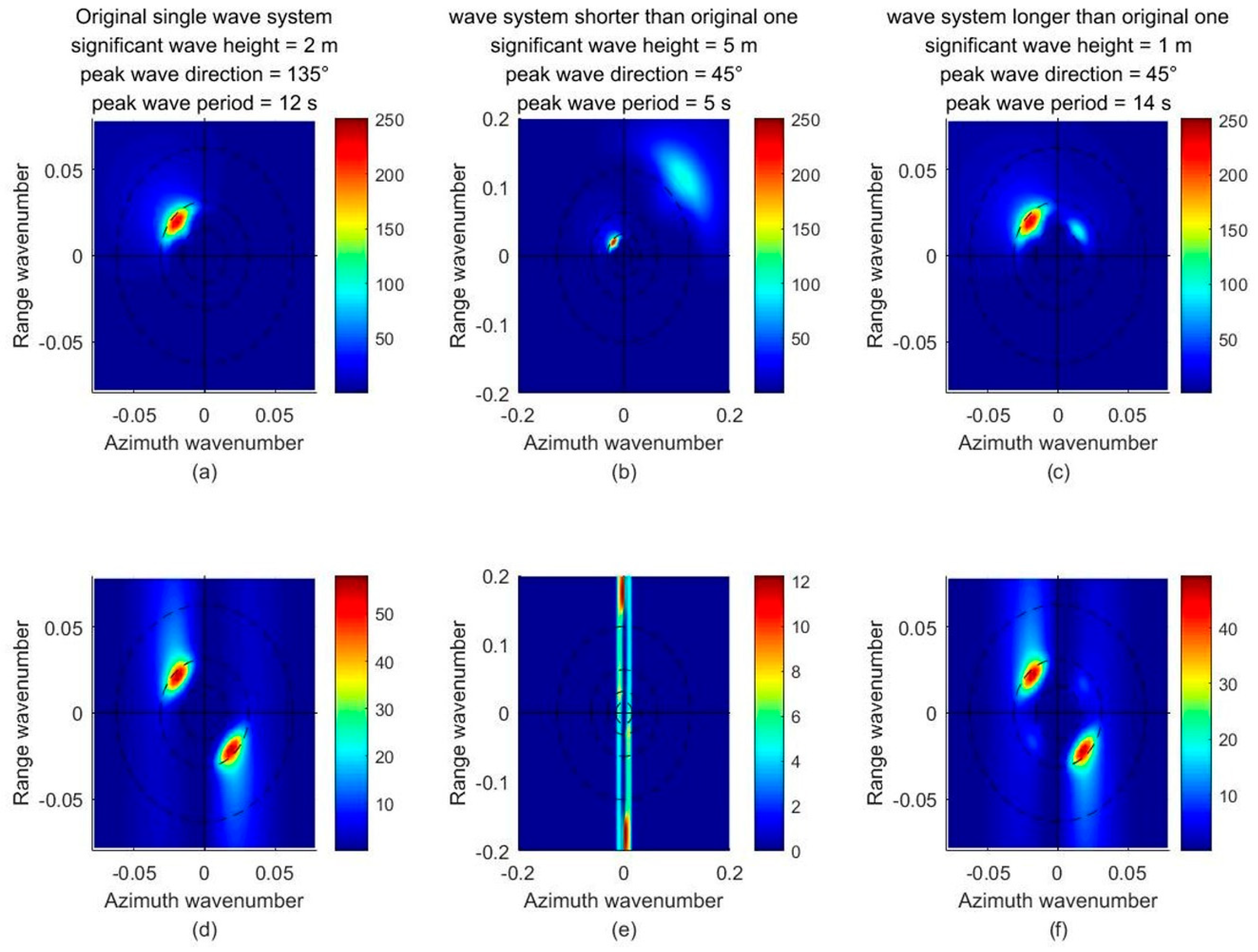
Figure 1. Buoy distribution and colors denote the matching-up Sentinel-1 data density.
Atmosphere 14 01272 g001
Figure 2. SAR images and spectra with different inhomogeneity parameters, significant wave heights, peak wave direction, and peak wave period. (ad) SAR VV-polarization sub-images with size 224 × 224. (eh) Corresponding SAR spectra.
Atmosphere 14 01272 g002
Figure 3. SAR spectra calculated by the nonlinear imaging function and the variation in peak magnitude in different significant wave heights, wave periods, and wave directions. (ad) Denote the results at different significant wave heights; (eh) denote the results at different wave periods; and (il) denote the results at different wave directions.
Atmosphere 14 01272 g003
Figure 4. Waves calculated by JONSWAP spectra and the sech2 angular spread function and SAR calculated by the nonlinear imaging function for (a,d) the original wave system, (b,e) adding another shorter wave, and (c,f) adding another longer wave. The titles describe information about the wave.
Atmosphere 14 01272 g004
Figure 5. Schematic diagram of how azimuth cutoff attenuates the original signal of ocean wave power density.
Atmosphere 14 01272 g005
Figure 6. Structures of ResNet: (a) residual block without pooling, (b) residual block with pooling, (c) complete ResNet34 with residual blocks.
Atmosphere 14 01272 g006
Figure 7. Flow diagram of the training process for the wind and wave parameters.
Atmosphere 14 01272 g007
Figure 8. Histograms of the wind and wave parameters for (ae) the training data set and (fj) the validation data set. The label on the x-axis shows the names of the wind and wave parameters.
Atmosphere 14 01272 g008
Figure 9. Comparison of buoy measurements and CNN results for different wind and wave parameters (ae) for the training data set and (fj) for the validation data set. The titles show the error parameters, and the axis label shows the parameters’ names.
Atmosphere 14 01272 g009
Figure 10. Histograms of the wind and wave parameters after the constrained homogeneity test for (ae) the training data set and (fj) the validation data set. The label on the x-axis shows the names of the wind and wave parameters.
Atmosphere 14 01272 g010
Figure 11. Comparison of buoy measurements and CNN results for different wind and wave parameters after the constrained homogeneity test (ae) for the training data set and (fj) for the validation data set. The titles show the error parameters, and the axis label shows the parameters’ names.
Atmosphere 14 01272 g011
Figure 12. Spatial distribution of (a) WaveWatch3 model significant wave heights and (b) significant wave heights retrieved from SAR by ResNet34 in the region near Hawaii on 16 March 2022.
Atmosphere 14 01272 g012
Figure 13. Comparison of annual temporal variation between ERA5 reanalysis data and ResNet34 inversion from SAR n 120.46° E 25.69° N in 2021 for (a) significant wave height, (b) mean wave period, and (c) wind speed.
Atmosphere 14 01272 g013
Figure 14. Spatial distribution of (a) significant wave height, (b) mean wave period, and (c) wind speed retrieved from SAR by ResNet34 on the west coast of North America on 20 December 2020. The solid circles are the CFOSAT measurements, and the circle’s color denotes the value of the corresponding parameter.
Atmosphere 14 01272 g014
Figure 15. Annual temporal variation comparisons between buoy measurements and ResNet34 inversion results for (a) significant wave height, (b) mean wave period, and (c) wind speed using SAR data pass the homogeneity test. (d) Shows a comparison of wind speed from buoy measurements and ResNet34 inversion results using all SAR data in 2020.
Atmosphere 14 01272 g015
Table 1. The wave parameters for different input waves.
Significant Wave Height (m)Wave Period (s)Wave Direction (°)
Original wave212135
Added long-wave11445
Added short-wave5545
Table 2. The validation results of error parameters for different parameters.
ParameterData NumberRMSEBiasSICOR
Significant wave height1190.58 m−0.01 m36%0.80
Mean wave period1190.92 s−0.14 s16%0.72
Mean wave direction11947°28%0.75
Wind speed1192.25 m/s−0.59 m/s51%0.22
Wind direction11969°72%0.17
Table 3. The validation results of error parameters for different parameters.
ParameterData NumberRMSEBiasSICOR
Significant wave height1220.45 m0.05 m24%0.90
Mean wave period1220.76 s−0.11 s12%0.88
Mean wave direction12239°−4°40%0.41
Wind speed1221.90 m/s0.01 m/s24%0.81
Wind direction12252°58%0.02
Table 4. The comparison of different wave parameter inversion methods using IW or SM mode data.
MethodData ModeCompared DataMatchingRMSE of Mean Wave Period (s)RMSE of Significant Wave Height (m)
Cutoff wavelengthSMBuoy20 m and 10 min1.860.69
CWAVE_S1-IWIWBuoy5–20 km and
interpolated in time
\0.55
CWAVE_EXIWWave model1/12–0.25° and
interpolated in time
0.910.57
Shallow CNNIWBuoy20 m and 1 h\0.32
This methodIWBuoy10 m and 1 h0.760.45
Disclaimer/Publisher’s Note: The statements, opinions and data contained in all publications are solely those of the individual author(s) and contributor(s) and not of MDPI and/or the editor(s). MDPI and/or the editor(s) disclaim responsibility for any injury to people or property resulting from any ideas, methods, instructions or products referred to in the content.

