Study on Seasonal Characteristics and Causes of Marine Heatwaves in the South China Sea over Nearly 30 Years

Abstract

Marine heatwaves (MHWs) are becoming more frequent and intense in many regions around the world, as well as in China’s marginal seas. However, the seasonal characteristics and associated physical drivers of MHWs are largely unknown. In this study, we analyze, based on multiple reanalysis and numerical model data, the seasonal characteristics and causes of MHWs in the South China Sea (SCS) over a near 30-year period (1991–2022). There exist significant seasonal variabilities in the spatiotemporal features and formation mechanisms of MHWs. MHWs in the SCS show significant increasing trends in terms of frequency, duration, and intensity. MHWs during the summer half-year are stronger than the winter half-year as a whole, with them being more likely to occur over the eastern SCS in the summer half-year and the western region in the winter half-year. However, the increasing trend of MHWs in the winter half-year exceed those in the summer. Additionally, we find that MHWs are associated with the unusually strong west Pacific subtropical high (WPSH) both in the summer and winter half-years. Nevertheless, the dominant factors for MHWs are different in the varied seasons. According to upper ocean temperature equation analysis, surface heat flux anomalies (especially shortwave radiation flux) are major effect factors in the summer half-year, while ocean dynamic processes play the main role in the winter half-year. An analysis of the typical MHWs also proves this conclusion. Moreover, MHWs occurring in winter are often accompanied by temperature anomalies within the mixed-layer depth. The findings imply that the formation mechanisms and space–time distribution of MHWs exist with a seasonal contrast in the SCS, rather than simply being due to large-scale circulation and flux anomalies. This may provide a useful reference for a deeper understanding and forecasting of MHWs under different seasons and weather.

1. Introduction

There has been a continuous warming of the global ocean and atmosphere since the Industrial Revolution [1], and it has significantly increased the frequency and intensity of extreme weather and climate events [2]. Compared with atmospheric heatwaves, marine heatwaves (MHWs) are extreme high-temperature events occurring in oceans at the weather or short–medium climate scale. In the last decade, as MHWs have become more common and widespread, people are starting to pay more attention to these newly discovered ocean phenomena.

MHWs are naturally occurring ocean phenomena that have been around for a long time. Events can persist for several months and span across thousands of kilometers. However, the discovery and definition of MHWs depend on high spatiotemporal resolution and long-time-scale observation data; thus, they have gradually attracted the attention of researchers in the recent decade [3,4,5]. From February to March 2011, the seawater temperature in the southwest coastal region of Western Australia rose to an unprecedented high value, and this high-temperature event was called by Pearce et al. a “marine heatwave” [5]. Since this concept was created, a great deal of research has been carried out on the definitions, spatiotemporal features, formation mechanisms, marine ecosystem impacts, and the variation trends in the MHWs of different regions and countries. For example, a continuous rise in sea temperature in the North Pacific Ocean from 2013 to 2015 (known as “Blob”) has severely affected local marine ecosystem and fishery resources [6]. In 2016, Australia’s Great Barrier Reef suffered a severe coral bleaching event due to the MHW that was driven by a strong El Niño event [7]. The duration and frequency of global MHWs have increased by 17% and 34% from 1925 to 2016, and there has also been a 54% increase in average occurrence days [8]. MHWs are also on the rise in the offshore area of China. In recent years, record-breaking MHWs have occurred in the Yellow Sea, Bohai Sea [9], East China Sea [10], and South China Sea [11,12]. In all of these cases, the global trend of frequent MHWs has attracted the attention of many scholars and government organizations.

MHWs are usually both affected by the internal variability in the global climate system and human activities, which lead to the complex formation mechanism and significant regional disparities. Holbrook et al. advise that long-duration MHWs mainly occur in the eastern equatorial Pacific Ocean and are always associated with El Niño events [13]. Oliver et al. also proved that MHWs in the eastern equatorial Pacific are significantly affected by ENSO, with the average duration being as long as 60 days [8]. On the other hand, the average duration of mid-latitude MHWs is 10–15 days. The occurrence of MHWs also exhibits certain seasonal characteristics [14]. MHWs are possible in all months, but there are significant disparities in the intensity, duration, and location between different seasons [15,16,17]. For certain species, the impact of MHWs during autumn and winter seasons is more pronounced. In addition, the mechanism of MHWs is highly intricate, and researchers have proposed factors such as atmospheric forcing (solar radiation and high-pressure systems) [11,12,18], ocean dynamic process (mixed-layer variation, upwelling, and mesoscale vortices) [19,20], etc. Li, Y. et al., through detailed analysis of the heat budget, show that the prediction of shortwave radiation flux and ocean dynamic term is an important factor affecting the accuracy of duration and intensity prediction [21]. Zhi, H. et al. show that early negative salinity anomalies at 100~150 m depth can make the mixing layer shallower, and the shallower mixing layer traps more heat in the upper water column, resulting in an increase in sea surface temperature (SST), thus enhancing the warm “Blob” [22]. However, the current understanding of the formation mechanism of MHWs in various sea areas remains limited, particularly in offshore regions where SST changes rapidly and is closely linked to anthropogenic activities.

The South China Sea (SCS) is a vast semi-enclosed marginal ocean basin situated in the southwest corner of the North Pacific Ocean (99°–125° E, 0°–25° N) with an average depth of 2000 m. The climate of the SCS is significantly influenced by monsoons, resulting in distinct seasonal variations [23]. The SCS boasts abundant fishery resources and coral reefs. However, in recent years, it has been impacted by MHWs, leading to severe damage to the ecosystem of the region. As a result, Chinese scholars have paid close attention to this phenomenon. Nevertheless, current research primarily focuses on summer months while placing greater emphasis on the mechanisms of atmospheric forcing and climate modes [11,12,24,25,26,27]. As mentioned above, it has been determined that the SCS is significantly impacted by monsoons in summer. However, there remains a lack of clarity regarding the potential differences in MHW characteristics across seasons and whether the importance of heatwave factors varies over time periods. To address these questions, this paper will conduct a diagnostic analysis that is based on the latest high-resolution observations and model data. In Section 2, we mainly introduce the diagnostic data and methods. The characteristics of MHWs in different seasons are detailed in Section 3. Next, the relationship between MHWs and the air–sea interaction flux is analyzed in Section 4. In Section 5, we separately select the typical cases of winter and summer half-year and then diagnose the factors with a mixed-layer temperature equation. Discussions and conclusions are included in Section 6.

2. Data and Methods

2.1. Definition and Index Calculation of MHWs

In terms of quality, MHWs are distinct and persistent anomalous warming events within the ocean. Generally, an extreme and high SST event is considered an MHW if the SST exceeds the ocean heatwave threshold for multiple consecutive days (as determined by Oliver et al. [3]). Currently, there are two widely accepted types of thresholds for MHWs in the academic community. The first type of threshold is a fixed temperature threshold, known as the absolute threshold. The second type involves selecting a threshold value that varies over time, referred to as the relative threshold. However, the detection capability of a fixed threshold and high-percentile temperature thresholds for ocean heatwave events during cold winters is limited. Therefore, the definition of MHWs proposed by Hobday et al. has been widely used in this research, which defines a marine heatwave as an event where the daily sea surface temperature in a specific region exceeds, for at least five consecutive days, the local seasonal threshold (i.e., the 90th percentile of SST during the same period in the climate reference period) [15]. If the interval between two events is less than 2 days, they are considered the same event. In this study, the climate reference period for MHWs spans from 1982 to 2011. The daily mean SST values within the same 11-day time window of the climate reference period were utilized to derive both the climate state value and the threshold value for each day, while a 31-day sliding average was computed. Marine heatwave calculations can be performed by using the Python program (Jupyter Notebook 6.4.12), which is available at http://github.com/ecjoliver/marineHeatWaves (accessed on 20 May 2022).

The MHW index is presented in

Table 1. Definition and calculation methodology of the MHW index [12,28].

Name of the Index	Definition	Calculation Methodology	Unit
HWN	Number of MHWs	$HWN=N$	Time
HWT	Total days of MHWs	$HWT={\sum }_{i=1}^N{D}_i$	Day
HWDU	Average duration of MHWs	$HWDU={\sum }_{i=1}^N{(D}_i)/N$	Day/Time
MHWI	MHWs intensity	$MHWI=T-\tilde{T}$	°C
HWI	Average intensity of MHWs	$HWI={\sum }_{i=1}^N{\sum }_{j=1}^{D_i}{(T}_{ij}-\widetilde{T_{ij}})/N$	°C/Time

, which encompasses frequency, duration, and intensity parameters [12,28]. The HWN is the number of times per year that the MHWs occur at each of the grid points. Similarly, HWT denotes the total duration of MHWs, HWDU indicates the average duration of each individual event, and HWI represents the average intensity of each MHW event. Here, we calculate the sum of the daily temperature anomalies exceeding the climatological mean intensity ($\tilde{T}$), which is represented by ${\sum }_{j=1}^{D_i}{(T}_{ij}-\widetilde{T_{ij}})$ and indicates cumulative intensity of an MHW event. Where i is the i-th event and j is the j-th day of an event, T_ij is the SST of the j-th day of the i-th event. The MHWI represents the daily intensity, which is calculated as the value of the SST for the day above the $\tilde{T}$.

2.2. Equation for the Temperature of the Upper Ocean

The variability of local SST was primarily influenced by thermal forcing and oceanic dynamic processes. The upper ocean temperature equation serves as an effective tool for quantitatively analyzing the impact of various factors on seawater temperature [29,30]. The upper ocean heat budget can be utilized to examine the process of MHWs from their onset and duration to their decline. The upper ocean refers to the water column above the mixed layer. The upper ocean temperature equation is derived from the conservation equations of heat and mass.

$$\frac{\partial T_H}{\partial t}=\frac{Q}{\rho C_{p}H}-\frac{1}{H}{\int }_{-H}^0\left(\mathbf{u}·{\nabla }_H{T}_H\right)dz-\left(w_H+\frac{dH}{dt}\right)\frac{T-T_H}{H}+\mathrm{r}\mathrm{e}\mathrm{s}\mathrm{i}\mathrm{d}\mathrm{u}\mathrm{a}\mathrm{l}$$

(1)

In this formula, the process of localizing the mixed-layer temperature represents the alteration of upper seawater. The subscript with an H indicates that the value is that of a physical quantity at the depth of the mixed layer. ρ denotes the mean density of seawater, Q is the net heat flux at the sea surface, Cp stands for specific heat capacity of seawater (usually 4096 J·kg⁻¹·°C⁻¹) [31], and H indicates the depth of the mixed layer. $w_H$ denotes the vertical velocity at the bottom of the mixed layer and T stands for the sea surface temperature. The depth of the mixed layer is the depth where the density increase compared to density at 10 m depth corresponds to a temperature decrease of 0.2 °C in local surface conditions. The first term on the right-hand side of the equation represents the contribution of net heat exchange between the atmosphere and ocean. The second term represents the contribution of horizontal advection to the heat balance of the mixed layer. This is calculated by vertically integrating the product of depth-dependent horizontal velocities and horizontal temperature gradients within the mixed layer. The third term represents the vertical transport. The residuals, which comprise smaller-scale processes such as heat diffusion and turbulent mixing, contribute to ocean temperature changes that fall below the resolution of the data. Reanalysis data will be utilized in this study to compute each component of the thermodynamic budget equation, with the aim of elucidating the physical mechanisms governing the temperature variations within the mixed layer and quantifying their respective contributions.

The definition of the latter two terms needs to be specifically elucidated here. In numerous prior studies on MHWs, these two terms have often been referred to as residual terms due to limitations in spatiotemporal data resolution [32,33]. However, subsequent research has prompted many scholars to argue that, under suitable conditions, the vertical terms should be considered separately, as there is intense turbulence below the surface mixed layer due to the strong shear and vertical mixing, or entrainment, which could still be important [34,35]. The vertical transport term in the equation represents vertical movement of seawater and entrainment effect caused by the wind field. When the wind blows across the ocean surface, it creates shear forces that cause the seawater to move and mix. To estimate vertical velocity, we assume that $w_H$ is zero at the surface and uniform at the base of the mixed layer. We will further explore the residual term in subsequent chapters.

2.3. EOF Analysis

In this paper, we use the Empirical Orthogonal Function (EOF) method to extract the principal model of MHWs and further correlation with other atmospheric factors. The basic idea of this method is to make orthogonal transformation of the initial data to separate the spatial modes and time coefficients that can cover the initial variable field information to the maximum extent. The spatial mode represents the basis function corresponding to the variance and reflects the spatial distribution of the element field. The time coefficient represents the time change characteristics corresponding to the spatial distribution mode. When the positive and negative signs are the same (or opposite) as the positive and negative signs of the corresponding mode, the change will be strengthened (or weakened), and the greater the absolute value of the coefficient, the more typical this type of mode is at this moment [36].

2.4. Data Sources

The daily mean SST data utilized in this study to examine the characteristics of MHWs were obtained from the National Oceanic and Atmospheric Administration (NOAA, Silver Spring, MD, USA), with a resolution of 1/4 degrees (https://psl.noaa.gov/data/gridded/data.noaa.oisst.v2.highres.html (accessed on 6 December 2023)). The dataset is derived from observations obtained via satellites, ships, and buoys. Following the adjustments for deviations, the optimal interpolation (OI) method was employed to interpolate the missing values [37]. The ocean reanalysis data employ the GLORYS12V1 product dataset provided by Copernicus Marine Services (Ramonville-Saint-Agne, France), featuring a spatial resolution of 1/12 degrees (https://data.marine.copernicus.eu/product/GLOBAL_MULTIYEAR_PHY_001_030/services (accessed on 6 December 2023)). The dataset comprises 50 layers of daily marine environmental variables, encompassing temperature, salinity, currents, sea surface height, and mixed-layer depth. Based on the real-time global prediction CMEMS system, the reduced order Kalman filter was utilized to assimilate the satellite altimeter data along the orbit, satellite sea surface temperature measurements, and thermohaline vertical profiles. Additionally, a 3D-Var scheme was employed to correct the large-scale deviations in the slow evolution of thermohaline properties. The data used for analyzing the heat flux and meteorological elements were derived from the ERA5 single-layer and multi-layer reanalysis data released by ECMWF, with a resolution of 1/4 degrees (https://cds.climate.copernicus.eu/cdsapp#!/dataset/reanalysis-era5-single-levels?tab=overview (accessed on 6 December 2023)). The dataset utilizes observations from more than 200 satellite instruments or conventional data, adopts the 4D-Var data assimilation method, and is reprocessed using several reprocessed satellite data-sets; thus, its accuracy is relatively high. The data utilized in the aforementioned analysis are gridded datasets with a regular latitude and longitude projection. The ETOPO2v2 global topographic data (with a resolution of 1/30°) used in this study were derived from the Global Relief Model developed by the National Geophysical Data Center (NGDC, Boulder, CO, USA), a subsidiary of NOAA, which includes both land and ocean topography (https://www.ngdc.noaa.gov/mgg/global/relief/ETOPO2/ETOPO2v2-2006/ETOPO2v2c/netCDF (accessed on 6 December 2023)).

3. Characteristics of MHWs in the SCS during Summer and Winter Half-Year

To investigate the seasonal disparities in the characteristics of MHWs between summer and winter in the SCS, we partitioned each year’s May to October as the summer half-year and November to April of the following year as the winter half-year. The SCS is strongly influenced by the monsoon, which further affects the mixed-layer seawater temperature by influencing the latent heat flux from the sea surface. When an event lasts from the previous half-year to the next, it will be divided into the longer half-year. If the two periods last the same number of days, they are divided into the previous half-year, mainly due to the concern about the event’s initiation. According to the calculation method presented in Table 1, we computed the average MHW Index (HWN, HWT, HWDU, and HWI) for each summer and winter half-year in the SCS from 1991 to 2022. The results are illustrated in Figure 1a–h, which is based on OISST datasets. Figure 1a–d represent the four indices of MHWs during the summer half-year, while Figure 1e–h correspond to those in the winter half-year. (1) From the perspective of occurrence frequency, the distribution of HWN in the South China Sea during the summer half-year was relatively homogeneous, with at least one occurrence of a severe MHW event observed annually throughout the entire sea area on average. During the winter half-year, the frequency of MHWs was lower than that in summer, and the average occurrence rate in the central-western region of SCS was less than once per winter half-year, which is significantly lower than other areas. (2) From the perspective of total occurrence days (HWT) and average duration (HWDU), significant spatial distribution differences also existed between summer and winter half-years. In the summer half-year, HWT and HWDU were primarily concentrated in the northern and central regions of the SCS, while, during the winter half-year, they were mainly found in the western region. The HWDU value at each grid point was obtained by dividing the HWT by HWN. In most sea areas, the average duration of MHW events during the summer half-year was approximately 15 days; meanwhile, in the areas surrounding the Xisha Islands and off the coast of Vietnam, it exceeded 20 days during the winter half-year. (3) According to the MHW intensity (HWI) index, the spatial distribution of HWI during the summer half-year is generally consistent with that of HWDU, with high values concentrated in the northern and central regions of the SCS at approximately 1.5 °C/time. The intensity of MHWs in the northern part of the SCS during the winter half-year exceeded that which was observed during the summer half-year, with maximum intensities occurring along the Beibu Gulf and Guangdong coastlines (where temperature anomalies can exceed 2 °C per event). Previous studies have shown that there are significant differences in the formation mechanisms of MHWs in different sea areas. However, there are certain differences in the characteristics of MHWs in different seasons in the SCS, which may be related to the seasonal basin-scale wind circulation in the SCS and the high-pressure weather system over the SCS.

Figure 2 illustrates the temporal evolution of the regional mean MHW magnitude and duration metrics, including HWN, HWT, HWDU, and HWI in the SCS from 1991 to 2022. Based on the chart analysis, it is evident that all stocks except for HWDU exhibit an upward trend, with HWN, HWT, and HWI showing particularly strong growth. This indicates that the occurrences of HMWs in the SCS have become more frequent and intense over the past three decades, regardless of season. According to the linear regression analysis of each index, with the exception of HWN, the upward trend (i.e., slope) of the other three indices during the winter half-year is greater than that observed during summer. This suggests that the upward trend in MHW intensity during the winter half-year is more pronounced than that observed during summer, which aligns with the recent changes in wintertime temperatures across the Northern Hemisphere.

4. Diagnostic Analysis of Factors Affecting MHWs in the SCS

Comparing the differences in the temperature change equation, based on contemporaneous thresholds, between periods with and without MHWs provides a more convincing analysis. We performed diagnostic analyses of the upper ocean temperature equations using the GLORYS12V1 and ERA5 datasets for the period 1993 to 2020 (this is the full period for which this ocean reanalysis dataset was published). As shown in Figure 3, daily averages were calculated for all variables in the equation under both MHWs and non-MHWs conditions. It can be found that the influence of the summer half-year on MHWs mainly depends on the heat forcing term. In the presence or absence of MHWs, the temperature changes are significantly different, i.e., about 0.03 °C/day. During the winter half-year, both the heat forcing term and residual term played equally important roles in influencing the sea surface temperature variability. The vertical entrainment term is positive both in summer and winter half-years, perhaps because of entrainment rate and mixing effect induced by the SCS monsoon. Due to the complexity of multi-scale ocean dynamic processes in the SCS and the resolution of the reanalysis data we used being only one twelfth of a degree, it is difficult to distinguish subtle processes below the vortex scale, whose contributions are likely to be contained in the residual term.

It is worth noting that despite the overall negative temperature trend during winter, the SCS as a whole is experiencing deheating. However, according to the definition of MHWs, this does not affect the delineation of events. Under the combined action of the atmosphere and the ocean, even during the period of temperature decline, it is still possible to rise above the threshold determined by the base period for 30 years, which will have an impact on the marine ecosystem. However, for a specific MHW event, different temperature tendencies can be used as an important reference for stage division.

4.1. The Identification of Representative Cases

According to previous research results, it is evident that, while MHWs during different seasons exhibit a correlation with atmospheric circulation anomalies, there exist distinct variations in their respective influence mechanisms. Hence, we opted for representative MHW occurrences and conducted a diagnostic analysis based on the upper ocean temperature equation. Referring to the methodology employed by Chen et al. in their investigation of the “Blob” phenomenon [32], the study area located in the central SCS has been selected for analysis, which is designated as R (refer to Figure 4a). The selection of region R is mainly based on the consideration that the SCS should be covered as much as possible, while the continental shelf should be covered as little as possible. The complex topography has a greater influence on the internal processes of the seawater and the results in the deep-water region are more representative. If we calculate MHWs based on the average SST of the whole SCS, many independent MHWs events occurring in local areas will be missed. According to the definition of an MHW, we have computed the threshold and incidence of MHW events from 2015 to 2020 (refer to Figure 4b). The green curve in these graphs represents the threshold, while the red area indicates the occurrences of the MHW events. The time period was chosen mainly because the more intense and persistent the MHWs are, the more robust they will be. And it is preferred that they are concentrated over a continuous period of time.

A total of six MHW events, denoted as S1–S3 and W1–W3, which occurred during the summer and winter halves, respectively, were selected. The corresponding occurrence time, maximum intensity, date of maximum occurrence, average intensity, and the duration of MHWs are presented in

Table 2. Refining the fundamental information of MHW incidents.

Half-Year of the Event	Name of the Event	Date of the Event	Maximum Intensity	Date of Maximum Intensity	Mean Intensity	Duration of Days
Summer half-year	S1	1 May 2016–28 May 2016	1.79 °C	19 May 2016	1.19 °C	28 days
	S2	17 May 2018–6 June 2018	1.45 °C	26 May 2018	1.10 °C	21 days
	S3	30 May 2020–27 September 2020	2.24 °C	17 September 2020	1.51 °C	121 days
Winter half-year	W1	25 October 2015–26 January 2016	2.04 °C	22 November 2015	1.35 °C	94 days
	W2	29 November 2016–12 January 2017	1.42 °C	16 December 2016	1.03 °C	45 days
	W3	20 November 2018–26 January 2019	1.87 °C	21 December 2018	1.34 °C	68 days

. Except for S3, which lasted 121 days, the winter MHWs exhibited a longer duration of events than that of the summer half-year. After analysis, the highest intensity of MHWs among the six events was recorded at 2.24 °C, while the lowest was at 1.42 °C. The average daily intensity remained above 1 °C throughout the event.

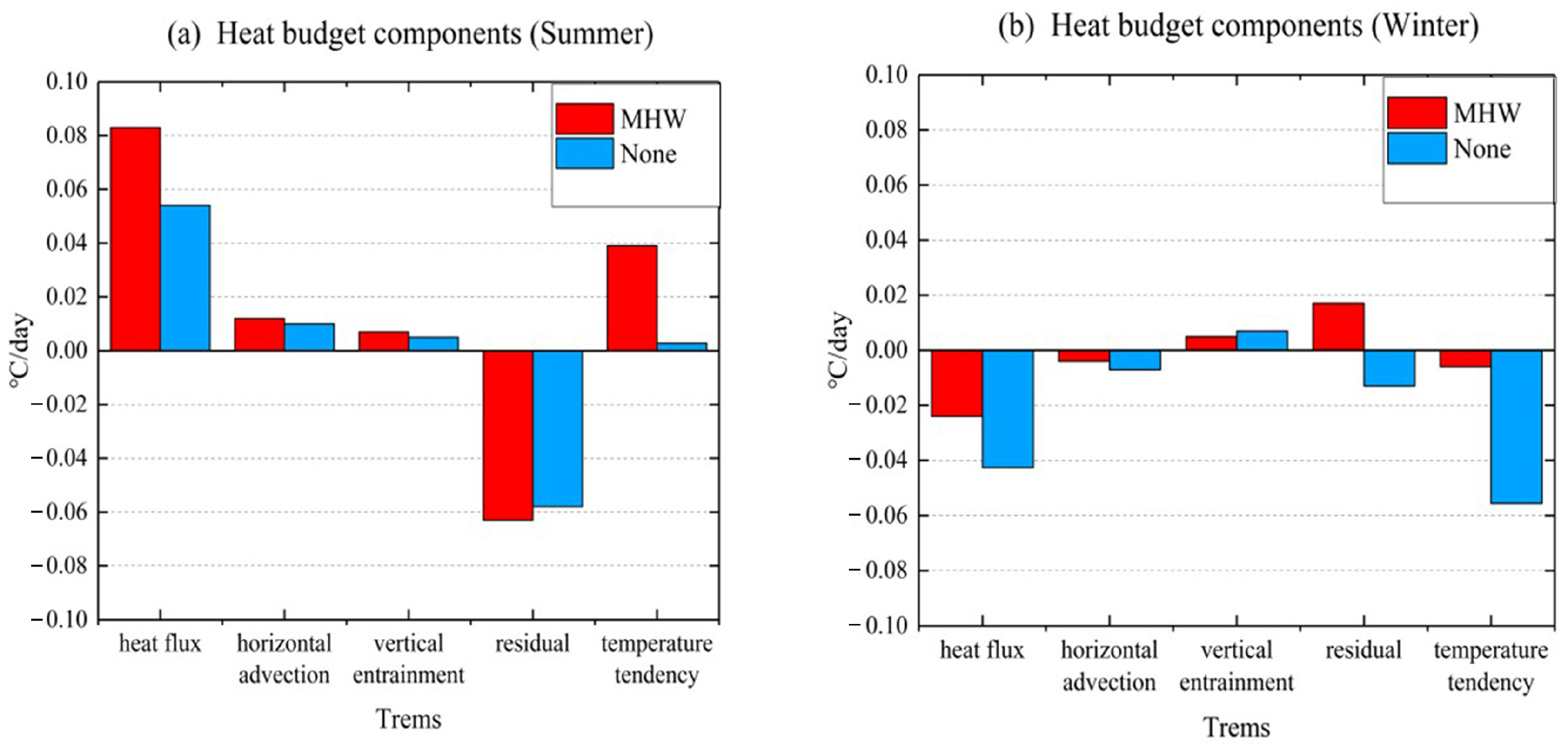
4.2. Diagnostic Analysis Based on the Heat Bugdet Equation of the Seawater Upper Ocean

According to the seawater temperature variation equation of the mixed layer, the local trend term of the mixed-layer temperature was decomposed into the sum of the net heat flux forcing term, advection term, vertical transport term, and residual term. We performed a time series analysis on the values of six marine heatwave events (S1–S3 and W1–W3), as depicted in Figure 5a,b. We then subsequently computed the cumulative average values for each event (refer to Figure 5c). The figure clearly illustrates the distinct role of each equation in the occurrence, development, maintenance, and extinction of every event. In the MHW events S1–S3, the heat flux term played a major role in the change in seawater temperature, and the mean heat flux can be as high as 0.13 °C/day, especially in S1. The net heat flux of the sea surface was primarily influenced by atmospheric forcing, thus leading us to conclude that the primary cause of the summer half-year MHWs in the SCS was due to atmospheric heat forcing. For the W1–W3 events during the winter half-year, there was minimal disparity in the magnitude of each term, indicating a certain degree of influence on SST fluctuations. The residual term exhibits a more pronounced negative value during the summer half-year, whereas the converse holds true in winter. In the W2 event, the residual term value of 0.07 °C/day significantly facilitated the increase in SST. This may be attributed to the heightened sub-mesoscale oceanic processes during winter, which induce reverse energy cascades and other conducive mechanisms for SST elevation. Insufficient data resolution precludes a detailed diagnostic analysis, but numerical simulation may provide further insight in the future. In conclusion, the combined influence of multi-scale ocean processes played a crucial role in determining the onset and cessation of that heatwave [38]. We can clearly observe that the factors influencing MHWs differ significantly between summer and winter half-years.

In addition, we conducted further analysis on the variations in temperature below the sea surface during MHWs. As depicted in Figure 6, these six MHWs occurrences were accompanied by anomalously high sea water temperatures near the mixed layer. Upon comparison, two significant characteristics have been identified: firstly, a positive correlation exists between the duration of MHWs and the magnitude of subsurface temperature anomalies, such as S3, W1, and W3 exhibiting stronger anomalies compared to the other three events; secondly, the sea subsurface temperature anomaly is notably stronger during winter than summer, with maximum amplitudes exceeding 3 °C in W1 and W3. Conversely, the subsurface temperature anomaly is relatively weak during the summer half-year. This indirectly supports the notion that dynamic oceanic processes are more vigorous during winter MHWs. In fact, the phenomenon of subsurface MHWs in the tropical western Pacific Ocean has been researched by S. Hu et al. [16]. The results of Figure 6 show that the continuous subsurface water warming anomaly in winter is accompanied by the gradual deepening of the depth of the mixed layer. This may be because there is a vertical upward heat transfer in the subsurface warm water, and the surface water continues to absorb heat, thus maintaining the persistence of MHW events. The thickness of the mixed layer has a certain influence on the diagnostic results, which is affected by the net heat flux term, which has been fully taken into account in the calculation formula. Here, we notice that the residual term is relatively large, nearly comparable to the temperature tendency. This will be discussed more in Section 6.2.

5. Influence of the Air–Sea Interaction on the MHWs in the SCS

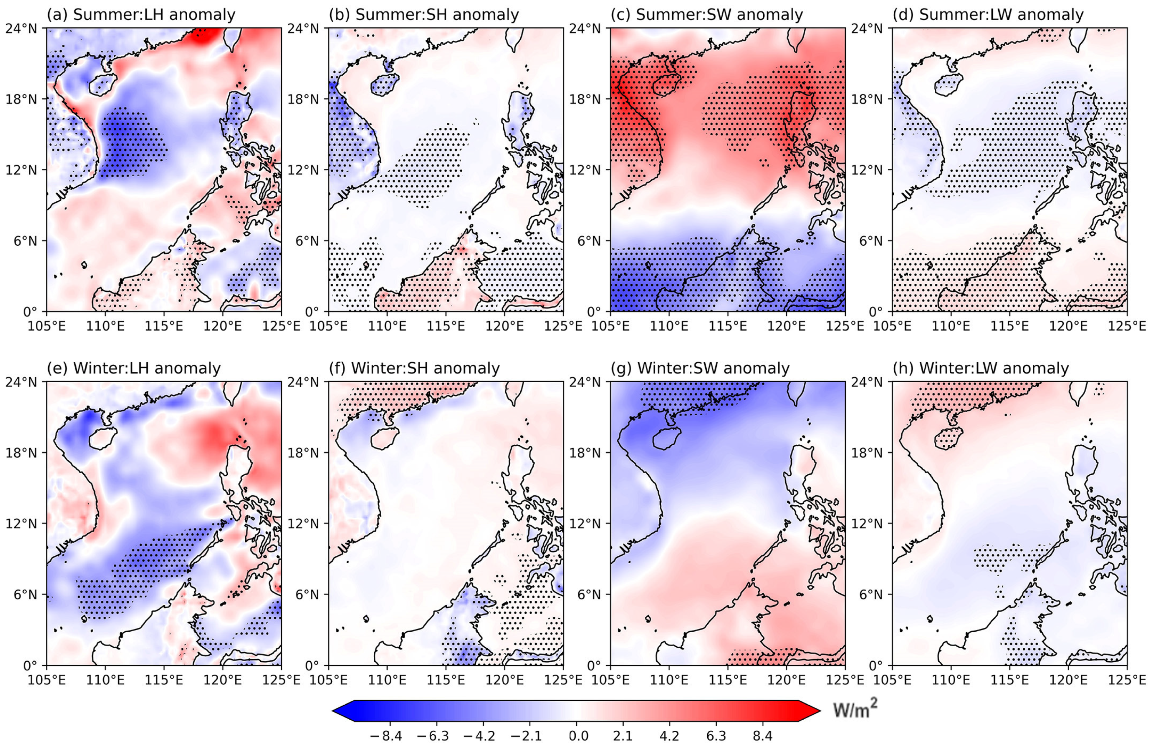
5.1. Diagnosis and Analysis of Ocean Surface Heat Flux

There exist intricate forcing and feedback mechanisms between the ocean and atmosphere, with the exchange in the air–sea heat flux serving as a crucial conduit. The net heat flux at the ocean surface is the summation of four factors: latent heat flux (LH), sensible heat flux (SH), shortwave radiation flux (SW), and longwave radiation flux (LW). It is considered positive when directed downwards. During the occurrence of six MHW events, the average anomalies in LH, SH, SW, and LW over the sea surface in R region were computed and summed up to derive the net heat flux anomalies (refer to Figure 7). It was observed that the outliers of shortwave radiation flux constitute the largest proportion among the outliers of net heat flux, followed by latent heat flux. In the summer half-year MHW events, there was a significant positive net heat flux, with shortwave radiation from the sun occupying a dominant position. According to the cumulative mean data, S1 exhibited significantly higher net heat flux anomalies than S2 and S3 during the summer half-year. This implies that short-term MHW events are primarily driven by a high contribution of shortwave radiation flux. During the winter half-year, both shortwave radiation and latent heat flux had a strong impact on the anomalous net heat flux. Additionally, the net heat flux exhibited a negative trend during the occurrences of MHWs. Coupled with the fluctuation in sea temperature, it can be deduced that the entire SCS is undergoing a process of cooling. Combined with the findings presented in Figure 7, a comprehensive analysis leads to the conclusion that the anomalous net heat flux of the sea surface (primarily shortwave radiation) played a significant role in driving the MHWs during the summer half-year in the SCS, particularly for brief events. Conversely, its impact on the winter half-year was relatively minor, because the increase in the depth of the mixed layer in winter (refer to Figure 6) made the cooling effect of heat flux on the sea water very limited.

5.2. The Correlation between MHWs and Sea Surface Heat Flux

To analyze the correlation between MHWs and meteorological elements, it is necessary to employ EOF technology for extracting their principal characteristics. According to the definition of MHWI, we utilized a daily OISST dataset for computation and reconstruction in order to produce daily sets of MHWI data. The main modes and corresponding time series of annual mean MHWI datasets were extracted by using the EOF decomposition method. Figure 8 depicts the spatial distribution of the primary modes of MHWI during summer and winter half-years, along with their corresponding time series (PCs). During the summer half-year, the first mode accounts for 71.2% of the total variance, while, during the winter half-year, it accounts for 61.97%, respectively. This suggests that the two modes are capable of effectively accounting for a majority of the variance and capturing the primary spatiotemporal features of MHWs.

The high-value region of the summer half-year Model 1 is primarily distributed in the eastern and southern regions of the SCS, including Zhongsha Islands, Nansha Islands, and their surrounding waters (refer to Figure 8a). The corresponding PC1 exhibits an increasing trend and significant decadal variability, with a clear inflection point around 2010 (Figure 8b). The winter half-year large value area of Model 1 is primarily distributed in the western waters of the SCS, encompassing the coast of Vietnam, Xisha Islands, Beibu Gulf, and their surrounding waters (Figure 8c). The interannual variation trend of the corresponding PC1 is similar to that of the summer half-year.

Then, we conducted a regression analysis on the winter and summer half-years’ MHWI first mode time series in order to investigate its correlation with the anomalies of LH, SH, SW, and LW flux (anomalies have been trended). As shown in Figure 9, overall, the MHWs during the summer half-year were strongly correlated with various heat fluxes, while, during the winter half-year, most of the ocean areas exhibited weak and insignificant correlations. During the summer half-year, there was a strong positive correlation between the shortwave flux from solar radiation (Figure 9c) and the MHWs in the northern and central SCS. This may be due to the enhancement of the west Pacific subtropical high (WPSH) anomaly and its westward extension, but further proof is needed. Under the control of the subtropical high, clear weather dominates with less cloud cover, resulting in more shortwave radiation received by the sea surface. The latent heat released by evaporation exhibits a negative correlation in the eastern waters of Vietnam (Figure 9a). Meanwhile, during MHWs, the elevated sea surface temperature leads to sensible and longwave radiative heat losses in the correlated areas, which also resulted in a negative correlation (Figure 9b,d). During the winter half-year, only the latent heat flux in the southern SCS showed a significant negative correlation, while the other factors were not significant. In the areas of boundary flow to the north and west of the SCS, there were particularly negative anomalies in the shortwave flux. This result indicated that the impact of heat flux on MHW events during the summer half-year is stronger than that during the winter.

5.3. The Association between MHWs and Large-Scale Atmospheric Circulation

According to prior research, the incidence of summer MHWs in the SCS is closely linked to anomalies in the large-scale atmospheric circulation. For instance, Yao et al. have indicated that the weakening of mid-western upwelling over the SCS during summer due to the influence of WPSH has facilitated the occurrence of MHWs [12]. Li et al. demonstrated a close relationship between the occurrence of MHWs and the near-surface stable anticyclone anomaly, which results in reduced cloud cover and increased solar radiation [11]. Is there a discrepancy in the impact of atmospheric circulation anomalies on the SCS’s MHWs during different seasons? To further analyze the issue, we conducted a regression analysis on the MHWI first mode time series of the summer and winter half-years, respectively, along with setting the meteorological elements at 500 hPa and 850 hPa. The significant grid points were marked with black dots through significance testing (Figure 10). Based on the data presented in Figure 10a,c, it can be inferred that the occurrence of MHWs during both summer and winter half-years was closely linked to the geopotential height at 500 hpa, as well as the anomaly strength of the WPSH. The position of the WPSH during the summer half-year deviated southward and westward from its climatological mean. Meanwhile, an anomalous strengthening and westward extension were observed in the winter half-year. According to the 850 hPa anomaly, an anticyclonic circulation anomaly was observed west of 130° E (corresponding to the WPSH), while, during the summer half-year, a cyclonic circulation anomaly was present east of 100° E and near the Tibetan Plateau. During the winter half-year, the cyclonic circulation remained anomalous, while there is no apparent anticyclonic circulation over the western Pacific. Additionally, notable disparities in wind direction were observed at lower altitudes during the months of the MHWs. The anomalies of the weather system have a profound impact on the occurrence of marine heatwave in the SCS. The weakening of the East Asian monsoon in winter will reduce the release of LH from the sea surface, and the strengthening of shortwave radiation caused by the high-pressure system in summer will increase the net heat flux of the ocean surface. The weakening of the southwest monsoon will affect the upwelling system along the coast of Vietnam, and the weakening of cold-water upwelling will further promote the generation of MHWs. Furthermore, the entrainment rate induced by the anomaly of wind stress may also affect the SST [35,39].

6. Conclusions and Discussions

6.1. Conclusions

Based on multi-source reanalysis and model data, the temporal and spatial characteristics of MHWs in different half-years over the SCS were computed. Through regression analysis, a correlation was identified between MHWs and anomalies in terms of atmospheric circulation and heat flux. Furthermore, we selected the individual cases of MHWs occurring during different months and conducted diagnostic analyses using the mixed layer temperature change equation to explore the factors influencing their occurrence and maintenance, as well as their seasonal variations. After comprehensive analysis, we obtained the spatiotemporal distribution characteristics and occurrence mechanisms of MHWs in the SCS over the past 30 years. The main conclusions of this study are summarized as follows:

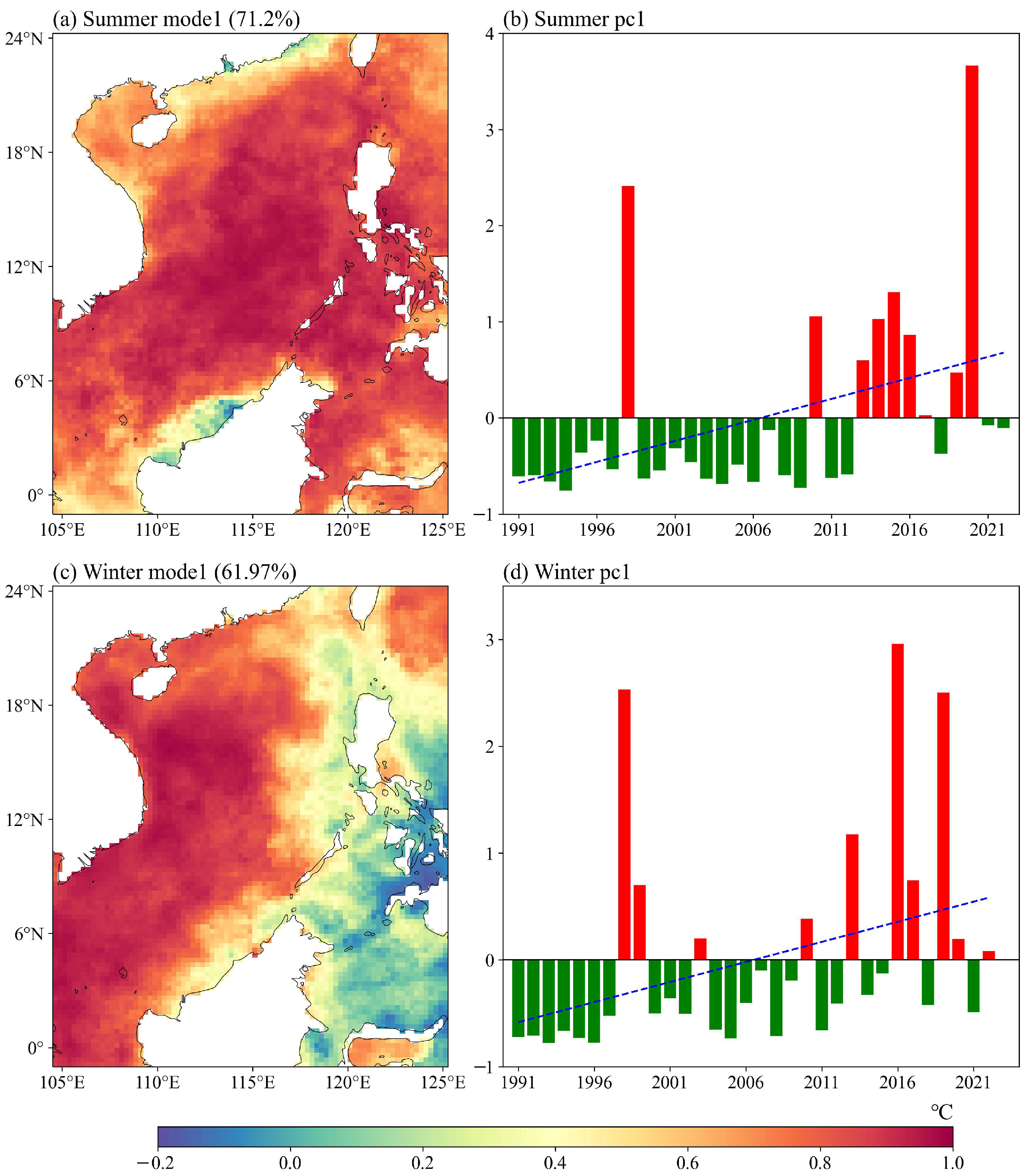
• The MHWs in the South China Sea exhibited distinct seasonal variations in both temporal and spatial characteristics. In general, the frequency and intensity of MHWs in the SCS have shown an increasing trend over the past 30 years. During the winter half-year, the frequency of MHWs was lower than that in summer, yet their intensity (mainly over the northern continental shelf) and duration (mainly over the western boundary currents) were higher than those in the summer. Furthermore, the trend of MHWs increasing in the SCS during the winter half-year is expected to surpass that of the summer. Through EOF decomposition of the daily MHWI dataset, we have identified that summer MHWs predominantly occur in the eastern and southern regions of the SCS, including the Zhongsha Islands, Nansha Islands, and their surrounding waters. Conversely, MHWs during the winter half-year are primarily concentrated in most western areas of the SCS, such as Vietnam’s coastlines, the Xisha Islands, Beibu Gulf, and the adjacent waters.
• From the perspective of air–sea interaction, MHWs in different seasons are closely linked to atmospheric circulation anomalies, particularly with respect to the impact of the WPSH pressure system. During MHW events, the subtropical high in the western Pacific exhibited abnormal westward extension and strengthening features. However, during the summer months, its large-scale circulation and wind field anomalies were even more pronounced. By means of regression analysis, it was found that the impact of sea surface heat flux on MHW events during the summer half-year was significantly more pronounced than that during winter. In most maritime regions, the correlation between anomalies in sea surface heat flux and MHWs during the winter half-year is weak and statistically insignificant. During summertime, when the ocean is heated, the low thermal inertia and shallow mixed-layer depth may cause the SST to respond rapidly.
• The diagnosis of individual cases and climate states, utilizing the mixed-layer temperature change equation, reveals significant differences in the factors influencing MHWs during the winter versus summer half-years. During the summer months, the primary factor influencing MHW occurrence remains the thermal forcing term. In contrast, during winter months, both thermal forcing and residual terms play equally important roles in affecting sea surface temperature variability. The atmospheric heat forcing was identified as the primary driver of MHWs in the SCS during summer months, while the internal dynamic processes were equally significant contributors to the events during winter. In addition, the prolonged heatwaves in the winter half-year are often accompanied by anomalies of elevated subsurface sea temperatures.

6.2. Discussions

MHWs have emerged as a significant challenge to the sustainable development of marine environments, ecosystems, and resources. In the context of global warming, MHWs are projected to increase in frequency, duration, and intensity across most regions of the world’s oceans. The MHWs in various sea regions across the globe exhibit significant differences, with distinct spatiotemporal characteristics and formation mechanisms. Despite ongoing research efforts, a comprehensive understanding of these features and mechanisms remains elusive. The research work presented in this article is a commendable attempt. However, the study area is limited and lacks comparative analysis with different datasets, thus exhibiting certain limitations. However, further research into the mechanisms of MHWs is imperative as it will facilitate a comprehensive understanding of this phenomenon and will enhance our ability to monitor, predict, and mitigate its impacts. Uncertainties in the heat budget estimate of the ocean arise from factors such as measurement errors, model representations, and the inherent complexity of the processes involved. Addressing these uncertainties requires improving observational capabilities, refining models, and accounting for the spatial and temporal variability of the different heat budget terms.

On the other hand, we must increase our focus on offshore MHWs. As a sensitive and vulnerable area of climate change in recent years, the offshore ocean will face greater risks and challenges. Therefore, it is crucial to attach great importance to and actively respond to MHW events and their impacts while establishing, as soon as possible, a systematic monitoring and forecasting mechanism for offshore warming water. Additionally, interdisciplinary collaboration is imperative in understanding the occurrence, impact, and adaptation of these events. Furthermore, it is required to alleviate the impact of extreme MHWs on offshore marine ecosystems, fishery resources, and socio-economic services, while providing support for climate change mitigation and for disaster prevention and reduction.

In addition, this paper also has certain limitations in terms of methodology and data. Firstly, the data used mainly consist of reanalysis and model data, which inherently have lower accuracy compared to observational data. Furthermore, we plan to compare our findings with data from Argo and Conductivity Temperature Depth (CTD) in order to discover new information. Secondly, the datasets we used to analyze heat budget are from different resources, which may lead to an imbalance between the different datasets. While it seems inevitable, as there are no complete reanalysis datasets that can cover all the atmosphere and oceans, judging from the results, the magnitude seems to be within a reasonable range. It is more convincing to use ocean–atmosphere coupled model data in the future. Additionally, the upper ocean temperature equation itself also has some limitations. For example, in this study, the residual terms calculated by this equation are relatively large. This is not an isolated incident, and it is common in other research [32,33,34]. The residual of the equation can be interpreted as being due to unresolved processes (e.g., diffusive mixing) and errors. For example, studies have shown that the inferred diffusivity at the base of the mixed layer is large (3 × 10⁻⁴ m²/s) and has a seasonal cycle [34]. The observations are examined for evidence of enhanced diapycnal mixing in the SCS, which reaches O (10⁻³ m²/s) in magnitude [40]. Therefore, the residual term is introduced to compensate for these unobserved or calculated energy terms, allowing conservation of energy to be satisfied. However, the larger values of the residual term may suggest that the accuracy of data needs to be improved or that we have not taken into account some important ocean dynamics and thermal processes. The active submesoscale process in the SCS in winter is also accompanied by the intensification of vertical heat flux, especially in late winter and early spring, which provides a considerable part of heat for the increase in mixed-layer temperature [41]. Unfortunately, it is hidden in the residual term and cannot be identified for the time being. Overall, uncertainties in the heat budget estimate of the ocean arise from factors such as measurement errors, model representations, and the inherent complexity of the processes involved. Addressing these uncertainties requires improving observational capabilities, refining models, and accounting for the spatial and temporal variability of the different heat budget terms.

References

1. Join, F. Climate Change 2022: Impacts, Adaptation and Vulnerability; Intergovernmental Panel on Climate Change: Geneva, Switzerland, 2022. [Google Scholar]
2. Robinson, A.; Lehmann, J.; Barriopedro, D.; Rahmstorf, S.; Coumou, D. Increasing heat and rainfall extremes now far outside the historical climate. NPJ Clim. Atmos. Sci. 2021, 4, 45. [Google Scholar] [CrossRef]
3. Oliver, E.C.; Benthuysen, J.A.; Darmaraki, S.; Donat, M.G.; Hobday, A.J.; Holbrook, N.J.; Schlegel, R.W.; Gupta, A.S. Marine heatwaves. Annu. Rev. Mar. Sci. 2021, 13, 313–342. [Google Scholar] [CrossRef] [PubMed]
4. Mills, K.E.; Pershing, A.J.; Brown, C.J.; Chen, Y.; Chiang, F.-S.; Holland, D.S.; Lehuta, S.; Nye, J.A.; Sun, J.C.; Thomas, A.C.; et al. Fisheries management in a changing climate: Lessons from the 2012 ocean heat wave in the Northwest Atlantic. Oceanography 2013, 26, 191–195. [Google Scholar] [CrossRef]
5. Pearce, A.F.; Lenanton, R.; Jackson, G.; Moore, J.; Feng, M.; Gaughan, D. The “Marine Heat Wave” off Western Australia during the Summer of 2010/11; Western Australian Fisheries and Marine Research Laboratories: Hillarys, WA, Australia, 2011. [Google Scholar]
6. Bond, N.A.; Cronin, M.F.; Freeland, H.; Mantua, N. Causes and impacts of the 2014 warm anomaly in the NE Pacific. Geophys. Res. Lett. 2015, 42, 3414–3420. [Google Scholar] [CrossRef]
7. Hughes, T.P.; Kerry, J.T.; Álvarez-Noriega, M.; Álvarez-Romero, J.G.; Anderson, K.D.; Baird, A.H.; Babcock, R.C.; Beger, M.; Bellwood, D.R.; Berkelmans, R.; et al. Global warming and recurrent mass bleaching of corals. Nature 2017, 543, 373–377. [Google Scholar] [CrossRef]
8. Oliver, E.C.; Donat, M.G.; Burrows, M.T.; Moore, P.J.; Smale, D.A.; Alexander, L.V.; Benthuysen, J.A.; Feng, M.; Gupta, A.S.; Hobday, A.J.; et al. Longer and more frequent marine heatwaves over the past century. Nat. Commun. 2018, 9, 1–12. [Google Scholar] [CrossRef]
9. Li, Y.; Ren, G.; Wang, Q.; You, Q. More extreme marine heatwaves in the China seas during the global warming hiatus. Environ. Res. Lett. 2019, 14, 104010. [Google Scholar] [CrossRef]
10. Oh, H.; Kim, G.-U.; Chu, J.-E.; Lee, K.; Jeong, J.-Y. The record-breaking 2022 long-lasting marine heatwaves in the East China Sea. Environ. Res. Lett. 2023, 18, 064015. [Google Scholar] [CrossRef]
11. Li, Y.; Ren, G.; Wang, Q.; Mu, L.; Niu, Q. Marine heatwaves in the South China Sea: Tempo-spatial pattern and its association with large-scale circulation. Remote Sens. 2022, 14, 5829. [Google Scholar] [CrossRef]
12. Yao, Y.; Wang, C. Variations in summer marine heatwaves in the South China Sea. J. Geophys. Res. Oceans 2021, 126, e2021JC017792. [Google Scholar] [CrossRef]
13. Holbrook, N.J.; Scannell, H.A.; Gupta, A.S.; Benthuysen, J.A.; Feng, M.; Oliver, E.C.; Alexander, L.V.; Burrows, M.T.; Donat, M.G.; Hobday, A.J.; et al. A global assessment of marine heatwaves and their drivers. Nat. Commun. 2019, 10, 2624. [Google Scholar] [CrossRef] [PubMed]
14. Hayashida, H.; Matear, R.J.; Strutton, P.G.; Zhang, X. Insights into projected changes in marine heatwaves from a high-resolution ocean circulation model. Nat. Commun. 2020, 11, 4352. [Google Scholar] [CrossRef] [PubMed]
15. Hobday, A.J.; Alexander, L.V.; Perkins, S.E.; Smale, D.A.; Straub, S.C.; Oliver, E.C.; Benthuysen, J.A.; Burrows, M.T.; Donat, M.G.; Feng, M.; et al. A hierarchical approach to defining marine heatwaves. Prog. Oceanogr. 2016, 141, 227–238. [Google Scholar] [CrossRef]
16. Hu, S.; Li, S.; Zhang, Y.; Guan, C.; Du, Y.; Feng, M.; Ando, K.; Wang, F.; Schiller, A.; Hu, D. Observed strong subsurface marine heatwaves in the tropical Western Pacific Ocean. Environ. Res. Lett. 2021, 16, 104024. [Google Scholar] [CrossRef]
17. Kuroda, H.; Setou, T. Extensive marine heatwaves at the sea surface in the Northwestern Pacific Ocean in summer 2021. Remote Sens. 2021, 13, 3989. [Google Scholar] [CrossRef]
18. Hamdeno, M.; Alvera-Azcarate, A. Marine heatwaves characteristics in the mediterranean sea: Case study the 2019 heatwave events. Front. Mar. Sci. 2023, 10, 366. [Google Scholar] [CrossRef]
19. Gao, G.; Marin, M.; Feng, M.; Yin, B.; Yang, D.; Feng, X.; Ding, Y.; Song, D. Drivers of marine heatwaves in the East China Sea and the south yellow sea in three consecutive summers during 2016–2018. J. Geophys. Res. Oceans 2020, 125, e2020JC016518. [Google Scholar] [CrossRef]
20. Xu, J.; Lowe, R.J.; Ivey, G.N.; Jones, N.L.; Zhang, Z. Contrasting heat budget dynamics during two La Nina marine heat wave events along northwestern australia. J. Geophys. Res. Oceans 2018, 123, 1563–1581. [Google Scholar] [CrossRef]
21. Li, Y.; Liu, J.; Lin, P.; Liu, H.; Yu, Z.; Zheng, W.; Chen, J. An Assessment of Marine Heatwaves in a Global Eddy-Resolving Ocean Forecast System: A Case Study around China. J. Mar. Sci. Eng. 2023, 11, 965. [Google Scholar] [CrossRef]
22. Zhi, H.; Lin, P.; Zhang, R.H.; Chai, F.; Liu, H. Salinity effects on the 2014 warm “Blob” in the Northeast Pacific. Acta Oceanol. Sin. 2019, 38, 24–34. [Google Scholar] [CrossRef]
23. Lau, K.; Yang, S. Climatology and interannual variability of the southeast asian summer monsoon. Adv. Atmos. Sci. 1997, 14, 141–162. [Google Scholar] [CrossRef]
24. Eakin, C.M.; Sweatman, H.P.; Brainard, R.E. The 2014–2017 global-scale coral bleaching event: Insights and impacts. Coral Reefs 2019, 38, 539–545. [Google Scholar] [CrossRef]
25. Tan, H.-J.; Cai, R.-S.; Wu, R.-G. Summer marine heatwaves in the South China Sea: Trend, variability and possible causes. Adv. Clim. Chang. Res. 2022, 13, 323–332. [Google Scholar] [CrossRef]
26. Liu, K.; Xu, K.; Zhu, C.; Liu, B. Diversity of marine heatwaves in the South China Sea regulated by enso phase. J. Clim. 2022, 35, 877–893. [Google Scholar] [CrossRef]
27. Wang, Y.; Zhang, C.; Tian, S.; Chen, Q.; Li, S.; Zeng, J.; Wei, Z.; Xie, S. Seasonal cycle of marine heatwaves in the northern South China Sea. Clim. Dyn. 2023, 61, 3367–3377. [Google Scholar] [CrossRef]
28. Wang, P.; Tang, J.; Sun, X.; Wang, S.; Wu, J.; Dong, X.; Fang, J. Heat waves in china: Definitions, leading patterns, and connections to large-scale atmospheric circulation and SSTs. J. Geophys. Res. Atmos. 2017, 122, 10679–10699. [Google Scholar] [CrossRef]
29. Stevenson, J.W.; Niiler, P.P. Upper ocean heat budget during the Hawaii-to-Tahiti shuttle experiment. J. Phys. Oceanogr. 1983, 13, 1894–1907. [Google Scholar] [CrossRef]
30. Huang, B.; Xue, Y.; Zhang, D.; Kumar, A.; McPhaden, M.J. The NCEP GODAS ocean analysis of the Tropical Pacific mixed layer heat budget on seasonal to interannual time scales. J. Clim. 2010, 23, 4901–4925. [Google Scholar] [CrossRef]
31. Yuchen, Z.; Zhang, X.; Zhang, J. Spatiotemporal characteristics and vertical heat transport of submesoscale processes in the South China Sea. Period. Ocean Univ. China 2020, 50, 1–11. (In Chinese) [Google Scholar]
32. Chen, Z.; Shi, J.; Liu, Q.; Chen, H.; Li, C. A persistent and intense marine heatwave in the northeast pacific during 2019–2020. Geophys. Res. Lett. 2021, 48, e2021GL093239. [Google Scholar] [CrossRef]
33. Schmeisser, L.; Bond, N.A.; Siedlecki, S.A.; Ackerman, T.P. The role of clouds and surface heat fluxes in the maintenance of the 2013–2016 northeast pacific marine heatwave. J. Geophys. Res. Atmos. 2019, 124, 10772–10783. [Google Scholar] [CrossRef]
34. Cronin, M.F.; Bond, N.A.; Farrar, J.T.; Ichikawa, H.; Jayne, S.R.; Kawai, Y.; Konda, M.; Qiu, B.; Rainville, L.; Tomita, H. Formation and erosion of the seasonal thermocline in the Kuroshio extension recirculation gyre. Deep.-Sea Res. Part II Top. Stud. Oceanogr. 2013, 85, 62–74. [Google Scholar] [CrossRef]
35. Jia, W.; Sun, J.; Zhang, W.; Wang, H. The effect of boreal summer intraseasonal oscillation on mixed layer and upper ocean temperature over the South China Sea. J. Ocean Univ. China 2023, 22, 285–296. [Google Scholar] [CrossRef]
36. Wilks, D.S. Principal component (EOF) analysis. In International Geophysics; Academic Press: Cambridge, MA, USA, 2011; Volume 100, pp. 519–562. [Google Scholar]
37. Reynolds, R.W.; Smith, T.M.; Liu, C.; Chelton, D.B.; Casey, K.S.; Schlax, M.G. Daily high-resolution-blended analyses for sea surface temperature. J. Clim. 2007, 20, 5473–5496. [Google Scholar] [CrossRef]
38. Dong, J.; Zhong, Y. The spatiotemporal features of submesoscale processes in the northeastern South China Sea. Acta Oceanol. Sin. 2018, 37, 8–18. [Google Scholar] [CrossRef]
39. Mao, J.; Wang, M. The 30–60-day intraseasonal variability of sea surface temperature in the South China Sea during May–September. Adv. Atmos. Sci. 2018, 35, 550–566. [Google Scholar] [CrossRef]
40. Tian, J.; Yang, Q.; Zhao, W. Enhanced Diapycnal Mixing in the South China Sea. J. Phys. Oceanogr. 2009, 39, 3191–3203. [Google Scholar] [CrossRef]
41. Zhang, Z.; Zhang, X.; Qiu, B.; Zhao, W.; Zhou, C.; Huang, X.; Tian, J. Submesoscale Currents in the Subtropical Upper Ocean Observed by Long-Term High-Resolution Mooring Arrays. J. Phys. Oceanogr. 2021, 51, 187–206. [Google Scholar] [CrossRef]
Figure 1. The annual mean distribution of the HMW index in the SCS over the past three decades (1991–2022) is depicted. (ad) illustrate the annual average distribution of HWN, HWT, HWDU, and HWI during the summer half-year, while (eh) present their corresponding annual average distribution during the winter half-year. The results are based on OISST datasets.
Atmosphere 14 01822 g001
Figure 2. Annual mean time series of the MHW index in the SCS over the last 30 years (1991–2022). (ad) illustrate the annual average trend of HWN, HWT, HWDU, and HWI during the summer half-year, while (eh) present their corresponding annual average trend during the winter half-year.
Atmosphere 14 01822 g002
Figure 3. The equation for the temperature change in the mixed layer of the SCS; the cumulative average value of MHWs and non-MHWs periods during summer (a) and winter (b) half-years from 1993 to 2020. The unit is °C/day.
Atmosphere 14 01822 g003
Figure 4. The R region was selected (a), and time series plots of the MHWs for the R region during 2015–2020 were generated (b). The base period average is shown as a blue line, with the SST indicated by a black line. The green curve represents the threshold, while the red shaded area indicates occurrences of the MHW events.
Atmosphere 14 01822 g004
Figure 5. Time series of each term in the mixed-layer temperature change equation during the six typical MHW events: (a) summer half-year and (b) winter half-year, as well as (c) their cumulative average values. The unit used is °C/day.
Atmosphere 14 01822 g005
Figure 6. The vertical profile of temperature anomaly during the six typical MHW events. Black line represents the mixed layer depth.
Atmosphere 14 01822 g006
Figure 7. Time series of the various heat fluxes during the six typical MHW events: (a) summer half-year and (b) winter half-year, as well as (c) their cumulative average values. The unit used is W/m2.
Atmosphere 14 01822 g007
Figure 8. The first mode of EOF decomposition for the intensity of the MHWs (shading: °C) over the SCS: (a,b) summer half-year and (c,d) winter half-year, along with their corresponding principal component time series.
Atmosphere 14 01822 g008
Figure 9. During the summer and winter half-years, a regression analysis was conducted on the anomalous heat flux of the sea surface and the main mode of marine heatwaves in the SCS. The columns from left to right represent the LH, SH, SW, and LW fluxes, respectively. The dotted area indicates regions with a confidence level exceeding 99%.
Atmosphere 14 01822 g009
Figure 10. Regression analysis of the dominant modes of atmospheric circulation anomalies and MHWs during the summer and winter half-year in the SCS. Figures (a,c) depict the 500 hPa geopotential altitude anomaly (shaded in gpm) and the characteristics of the WPSH. The green line represents the climatological isolines at 5870 and 5880 gpm, while the blue line shows the monthly mean isolines under similar PC1 conditions (i.e., during MHWs). The representation of the 850 hPa geopotential height (shadow: gpm) and wind field (vector: m/s) by (b,d), respectively, is anomalous. The dotted region corresponds to the area that has been tested with a confidence level of 99%.
Atmosphere 14 01822 g010