
Evaluation of the Performance of the WRF Model in a Hyper-Arid Environment: A Sensitivity Study

 , , ,
, , ,  , , ,
, , ,
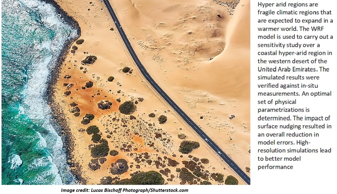
Abstract
:
1. Introduction
2. Materials and Methods
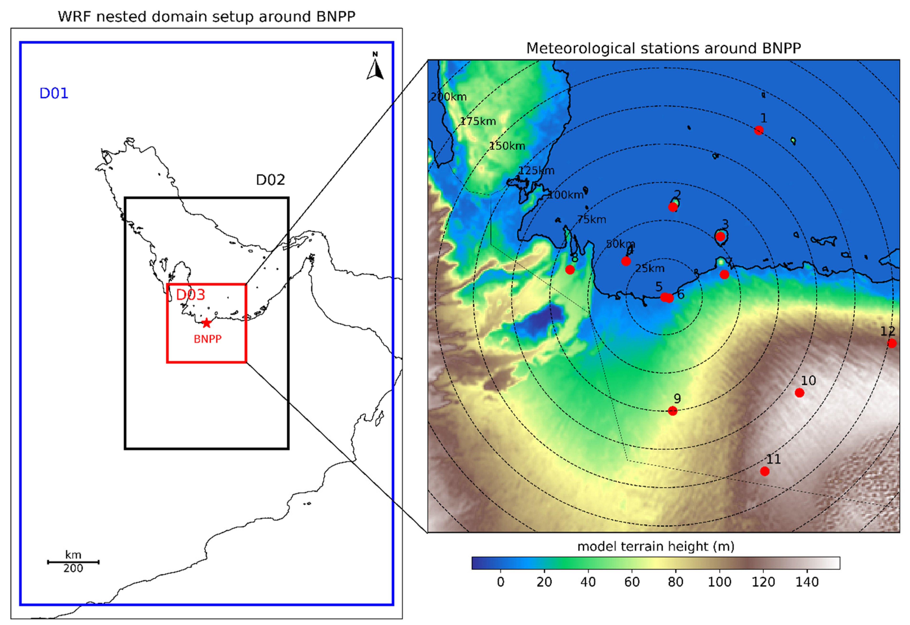
2.1. Study Area and In-Situ Measurements
2.2. Meteorological Model
2.3. Experimental Sensitivity Design
2.4. Error Metrics for Model Validation
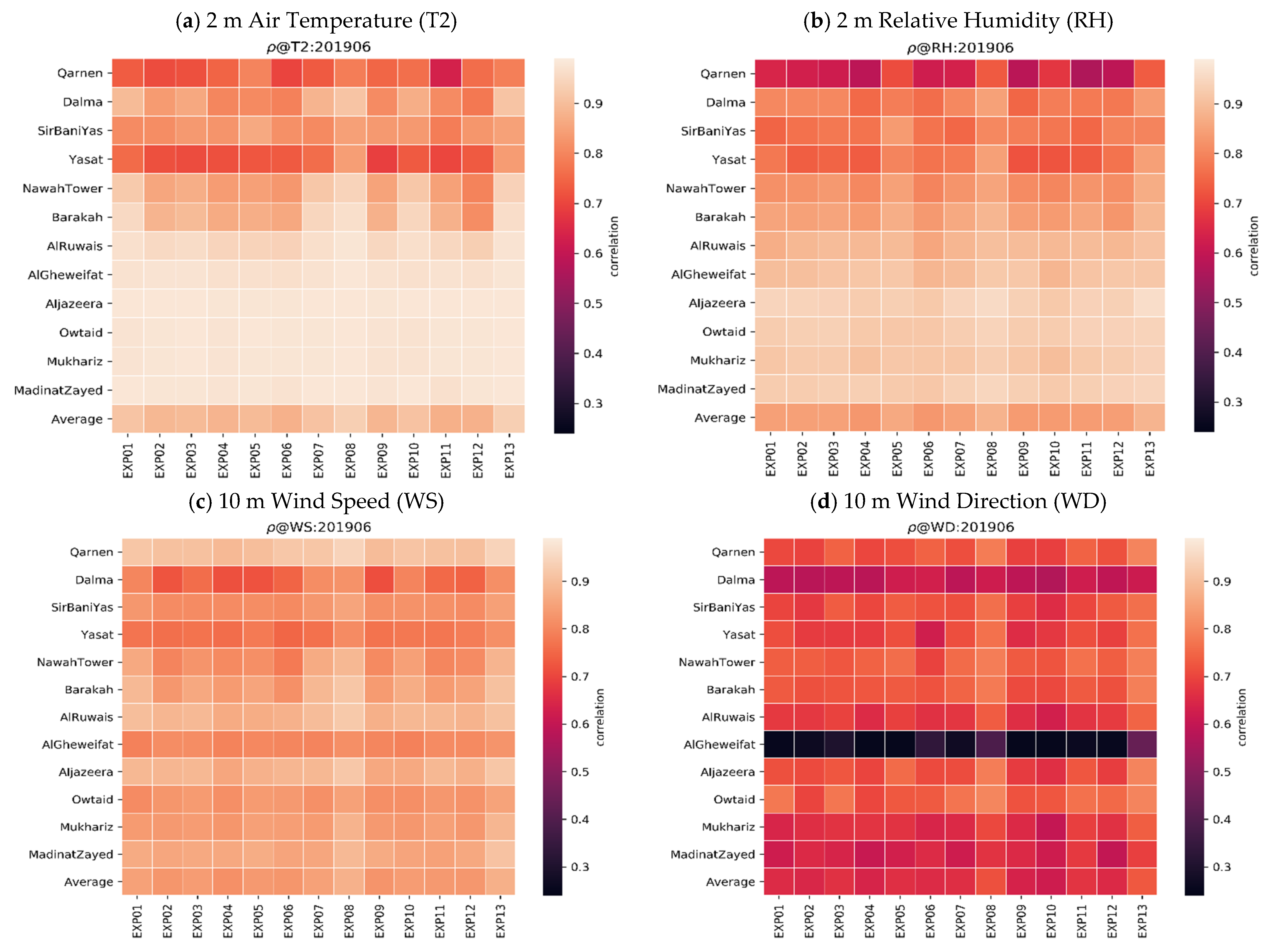
- the unbiased Pearson correlation coefficient (ρ)
- the Root Mean Square Error (RMSE)
- the Mean Absolute Error (MAE)
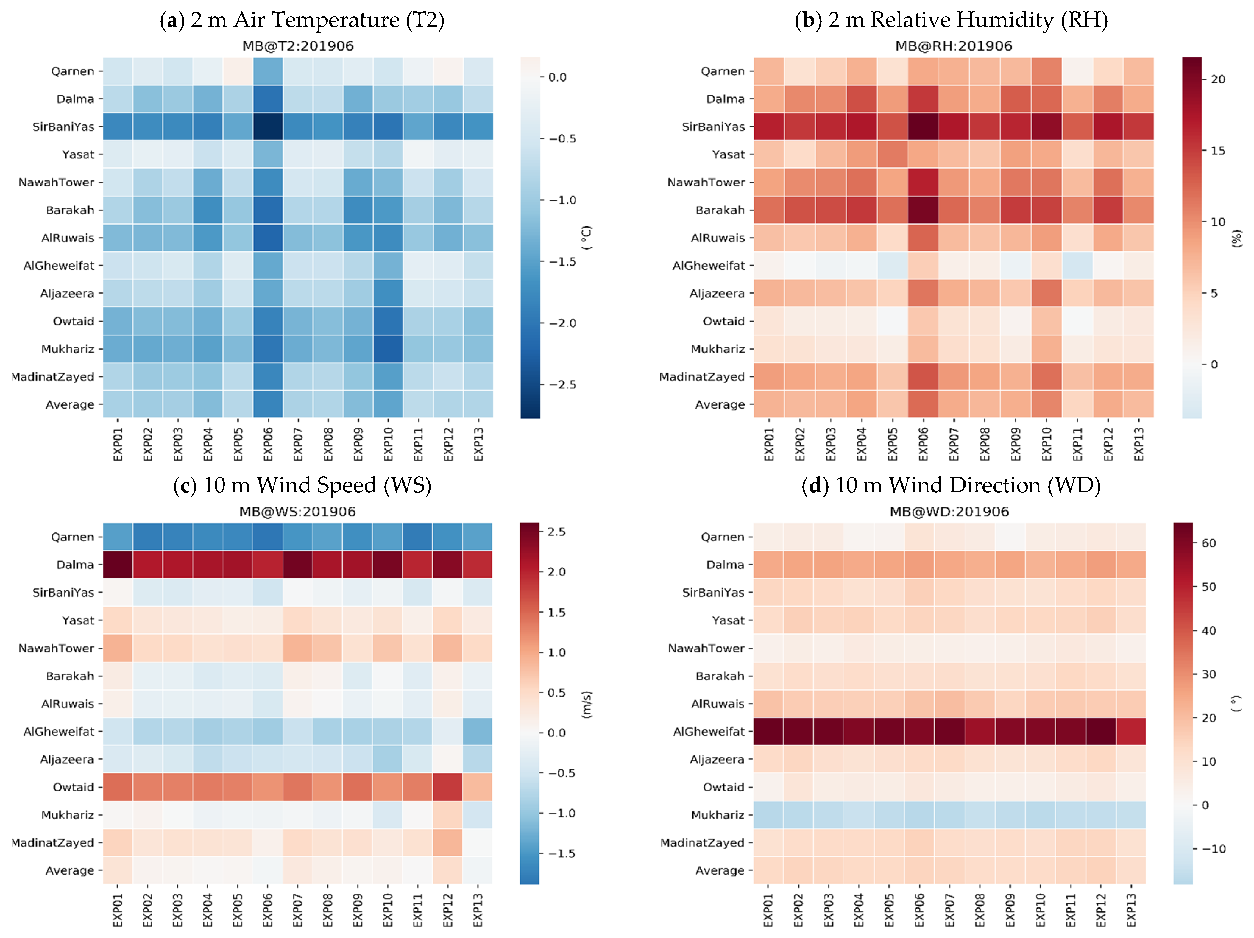
- the Mean Bias (MB)
- the Standard Error (STDE)
3. Results and Discussion
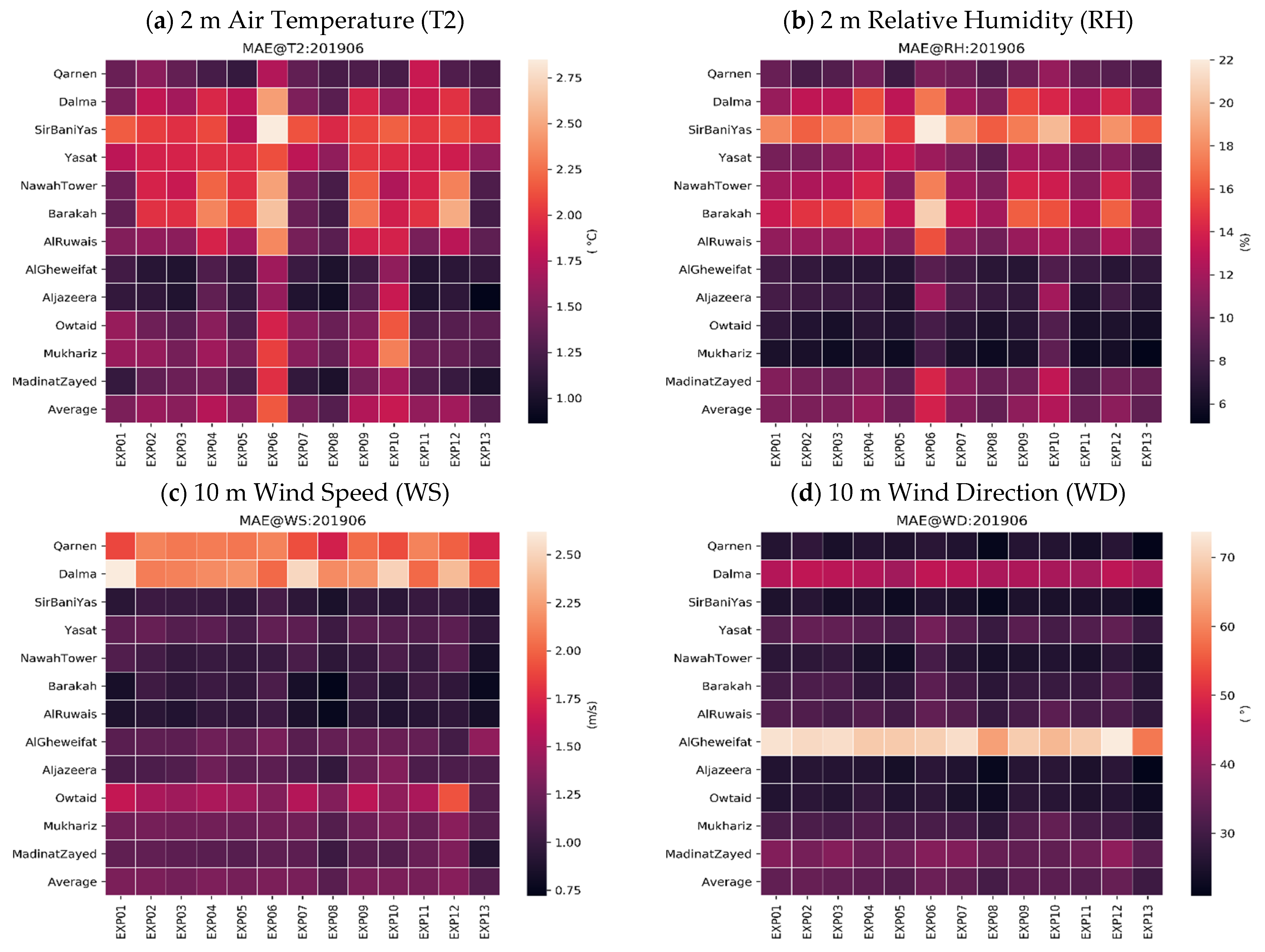
3.1. Overall Model Performance Assessment
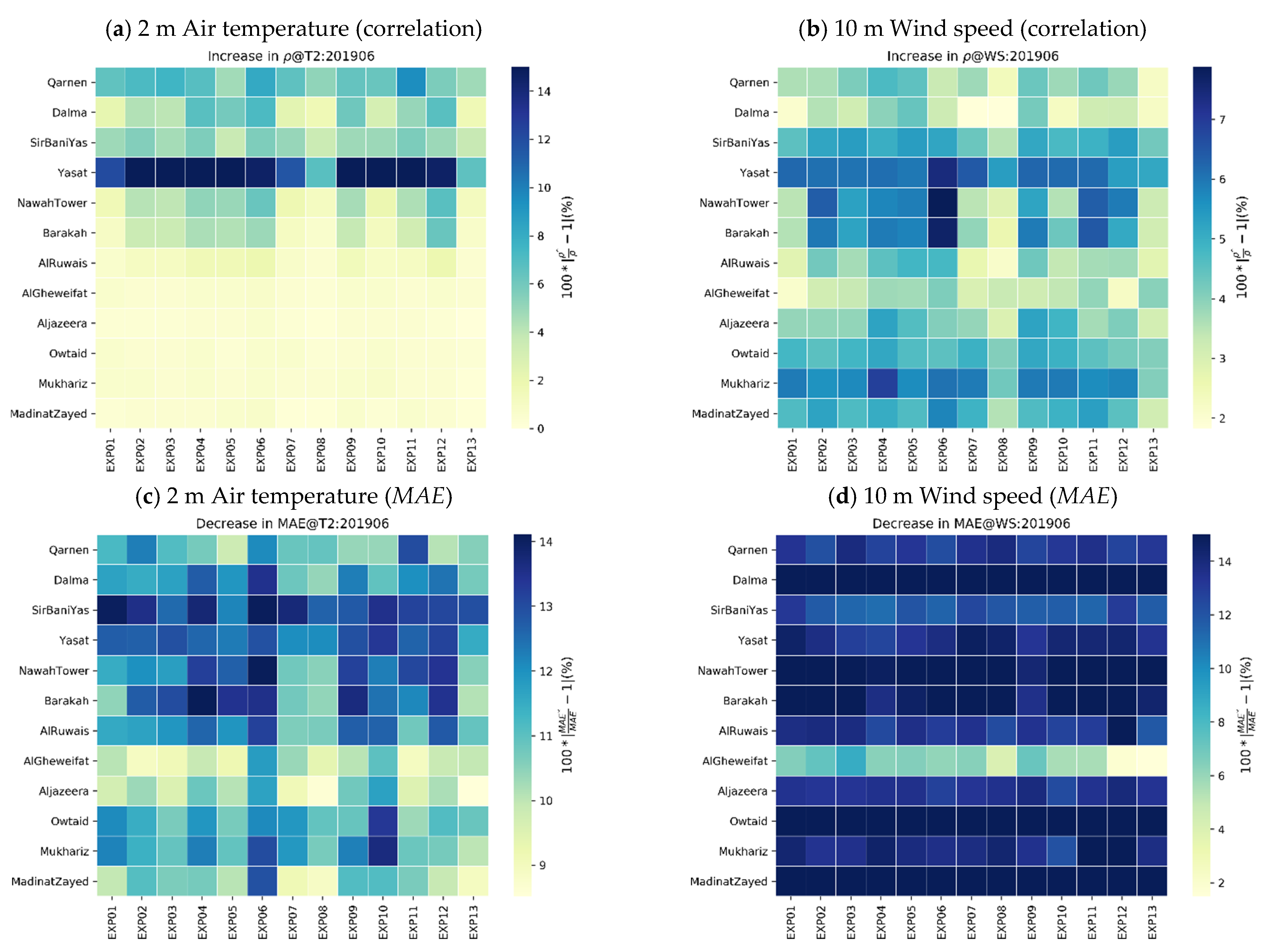
3.2. Impact of Station Nudging
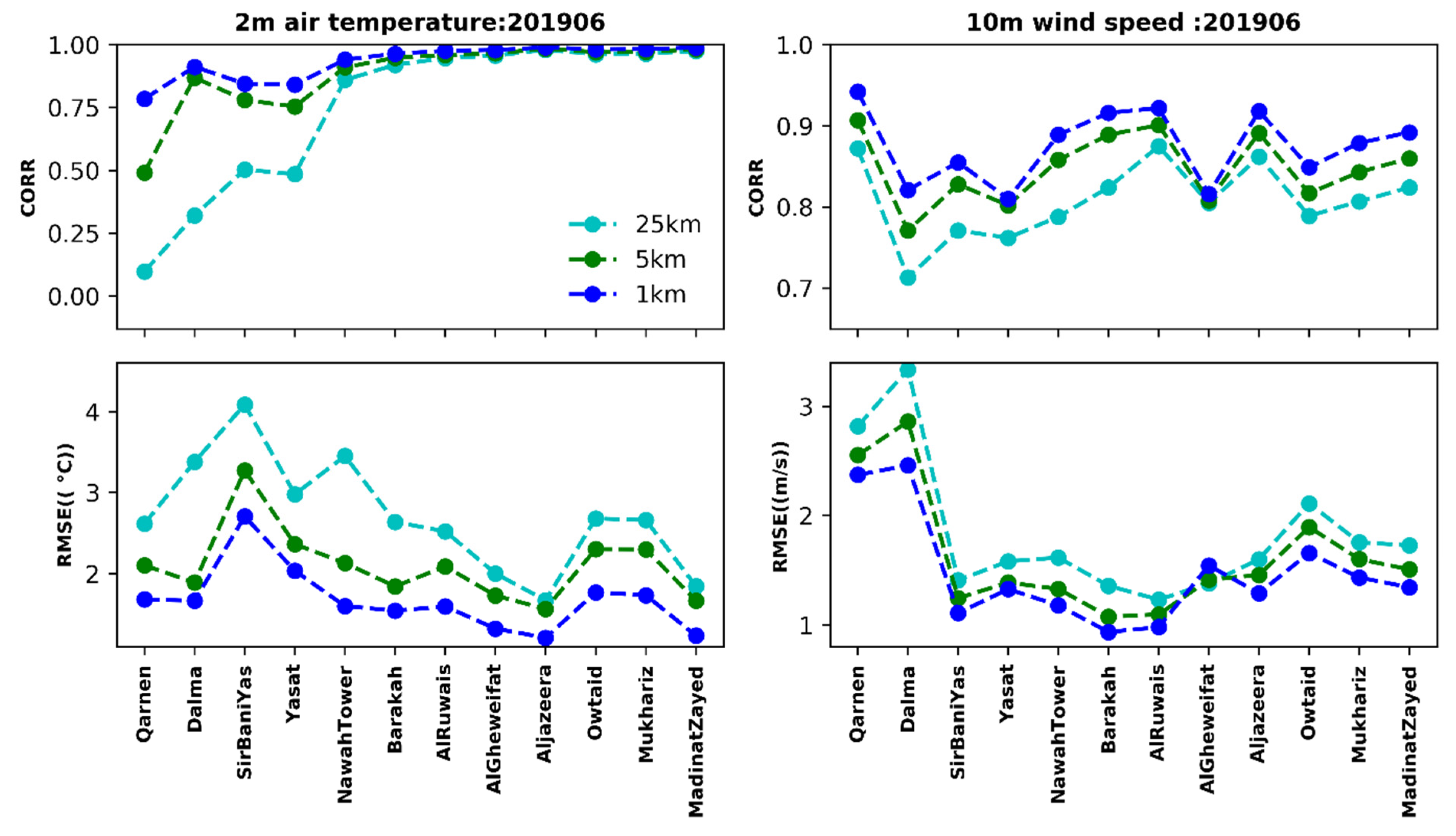
3.3. Sensitivity to Horizontal Resolution
3.4. Statistical Model Evaluation at Barakah Station
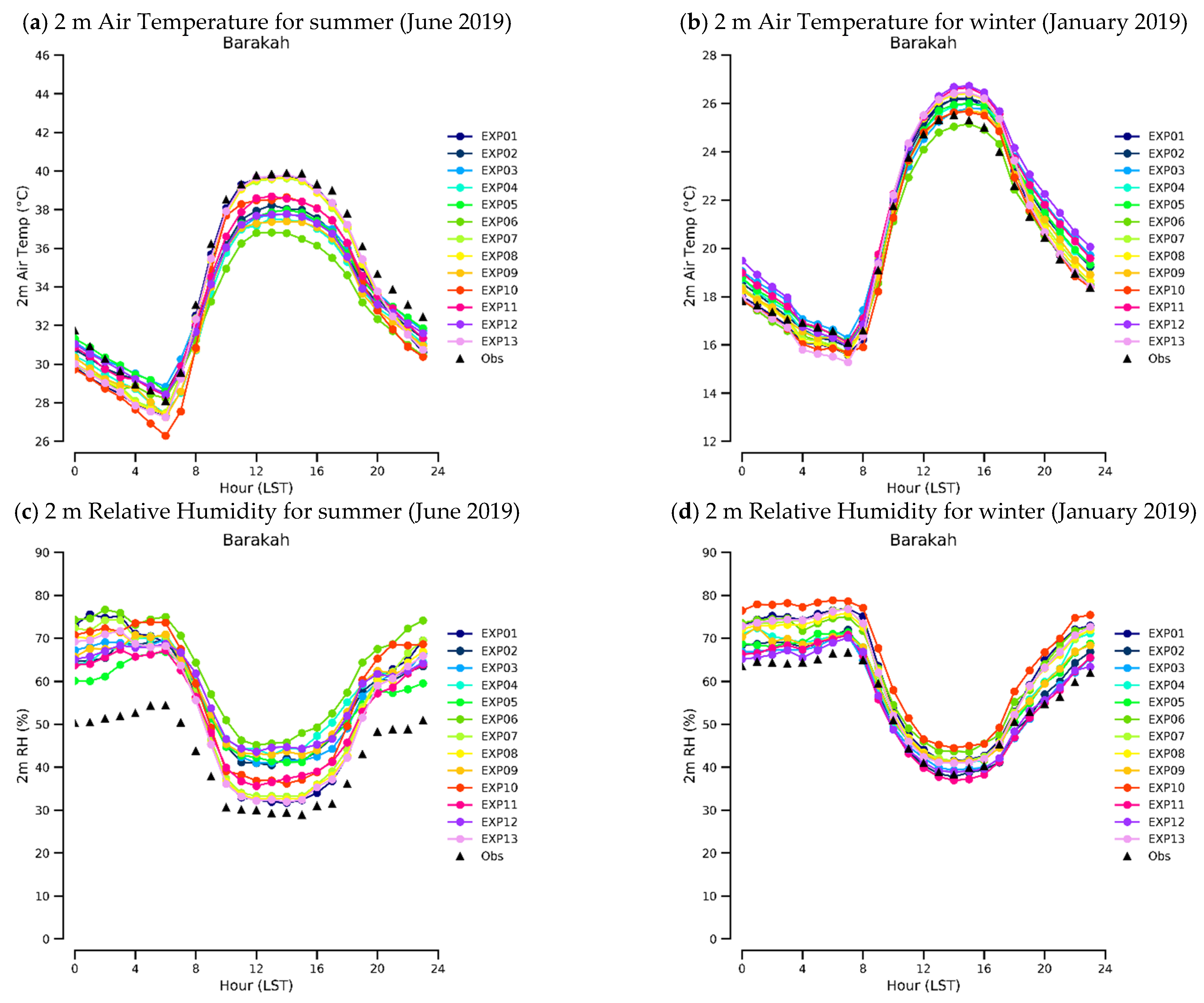
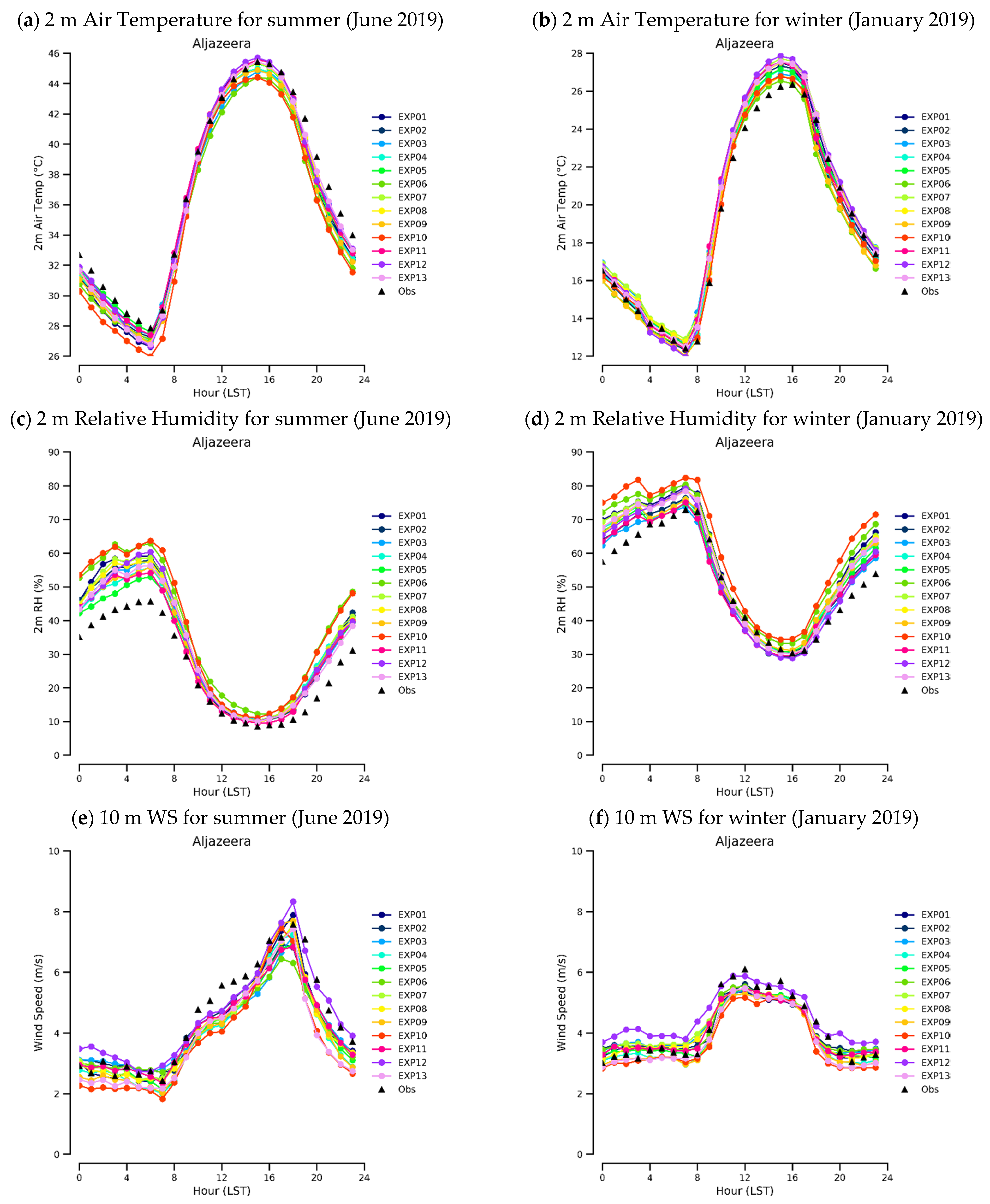
3.4.1. Air Temperature and Relative Humidity
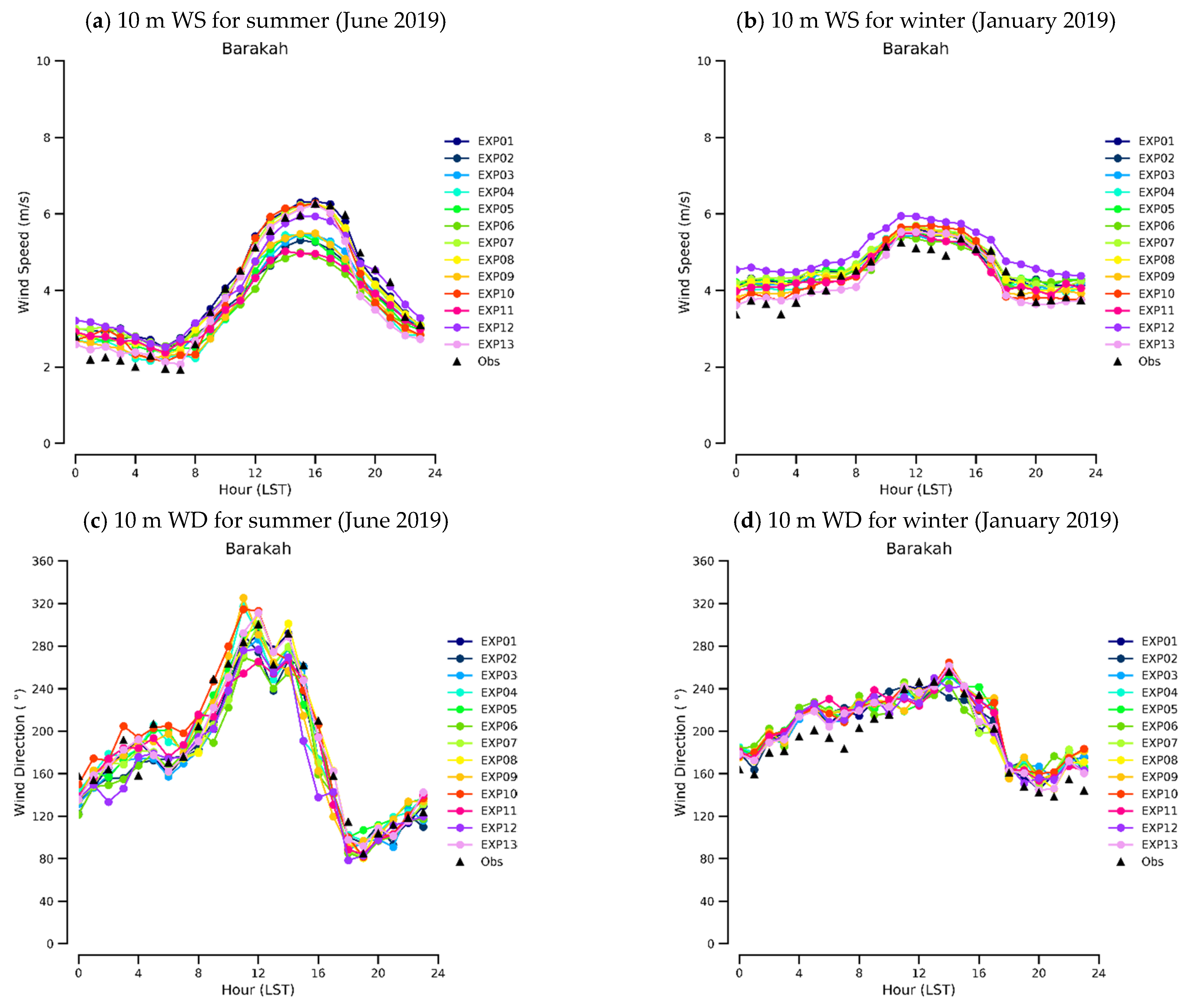
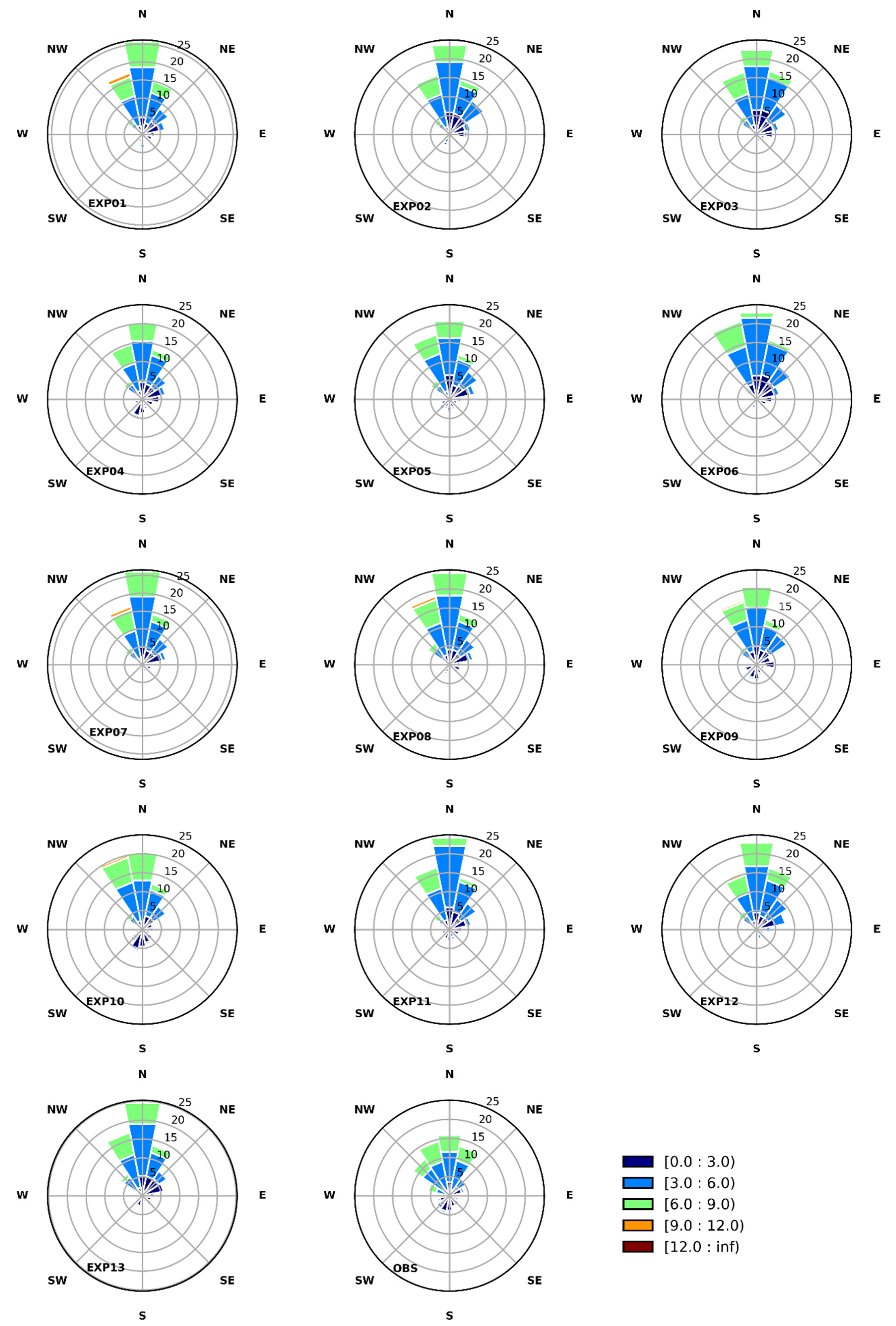
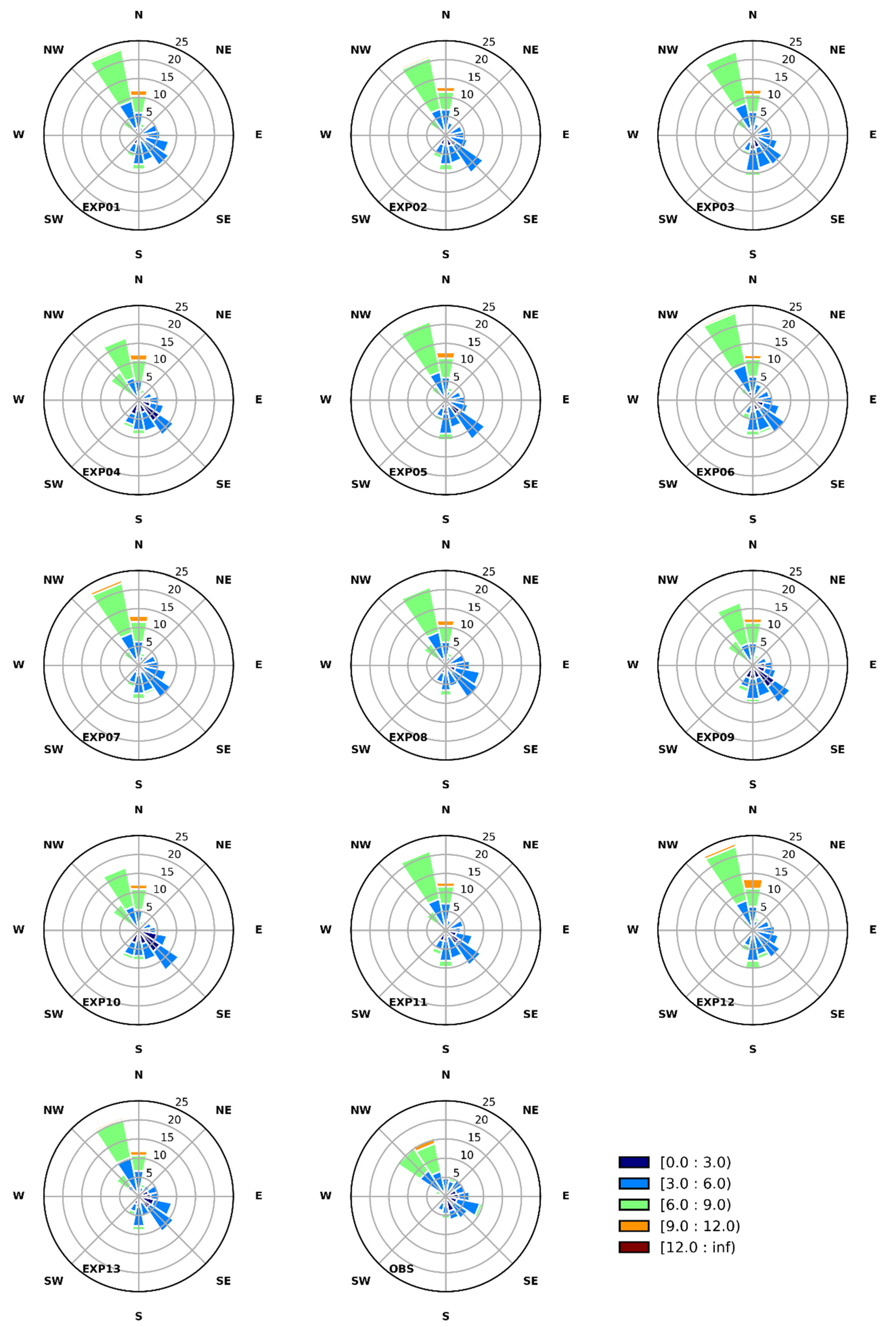
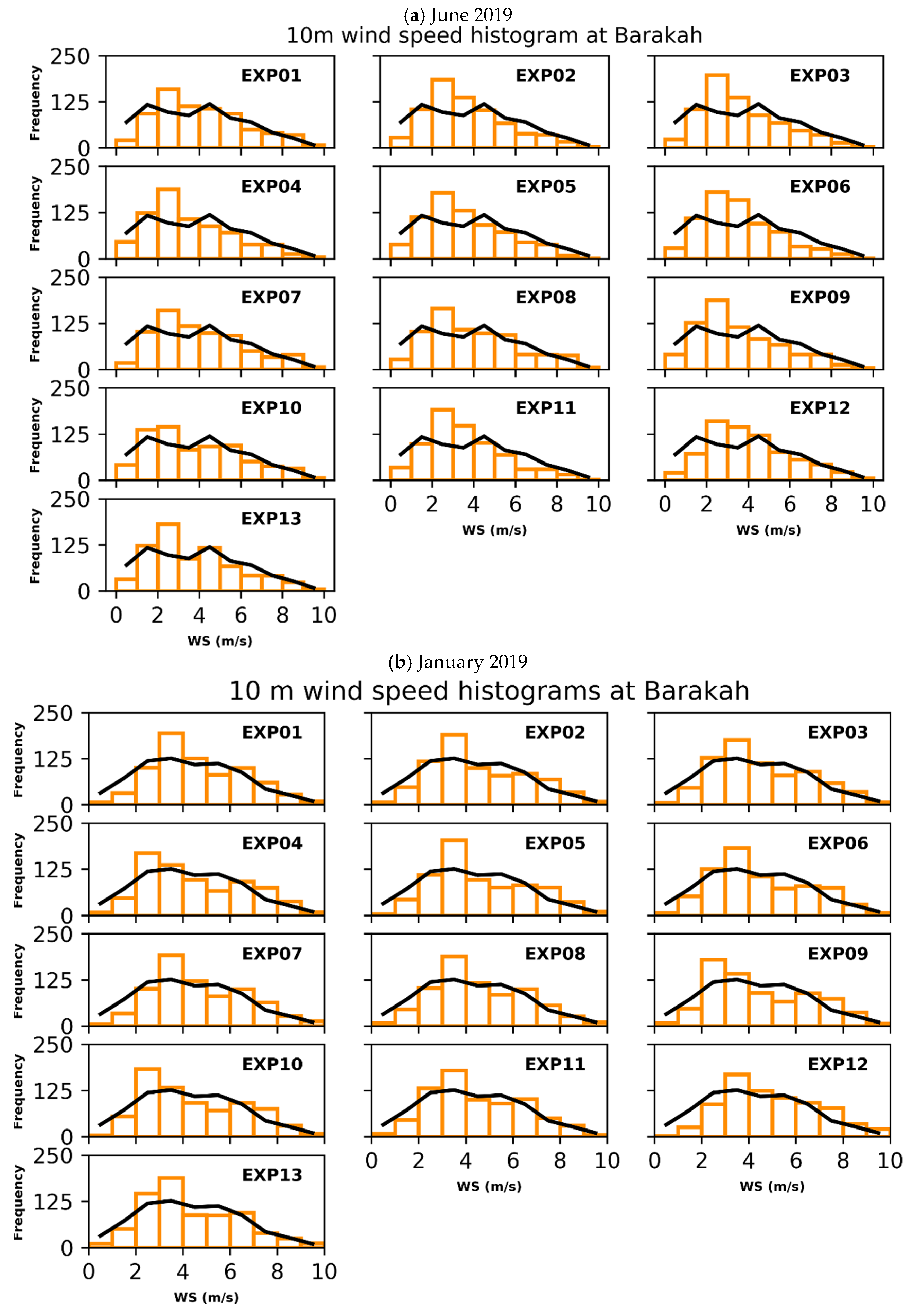
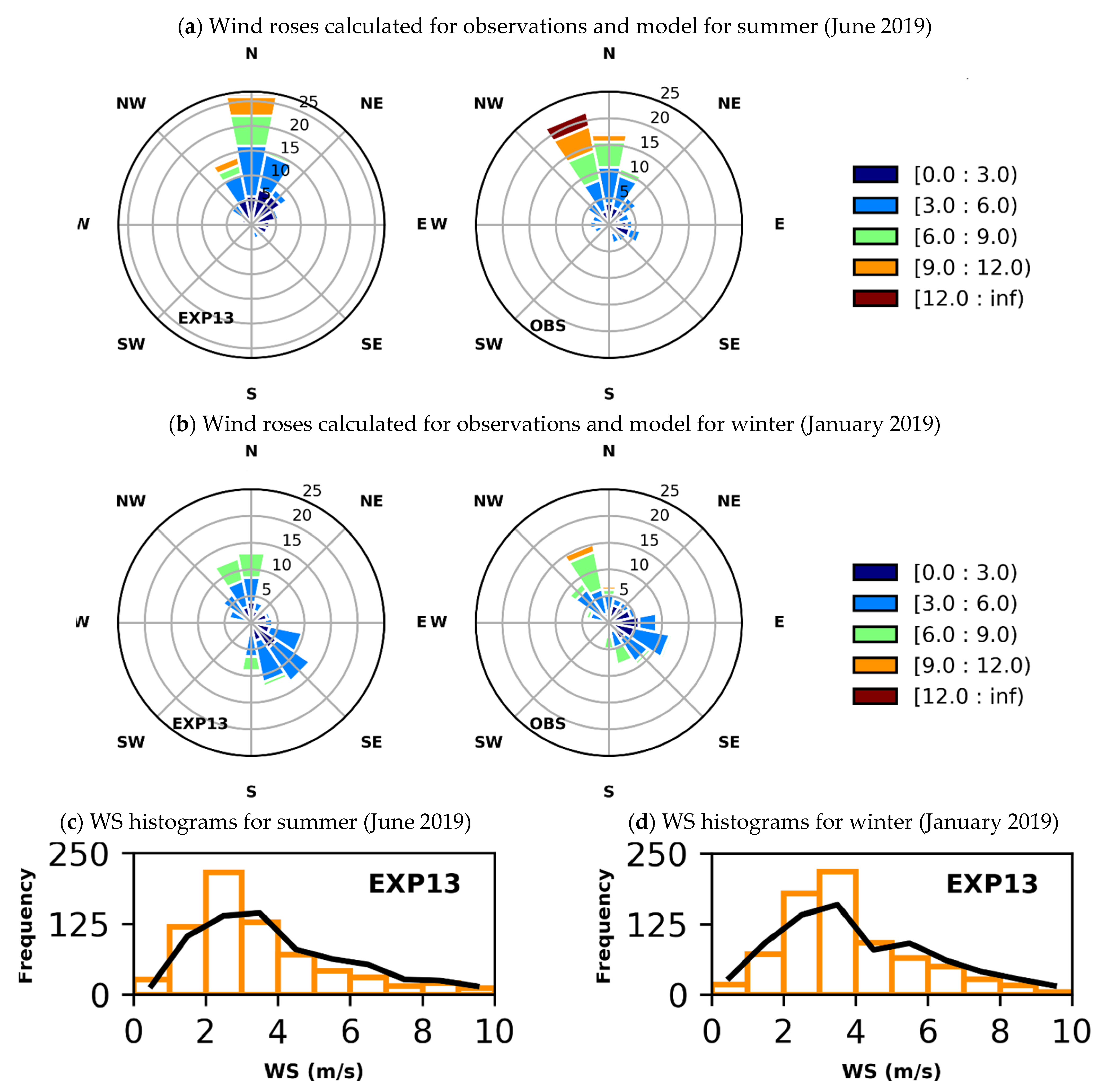
3.4.2. Wind Speed and Direction
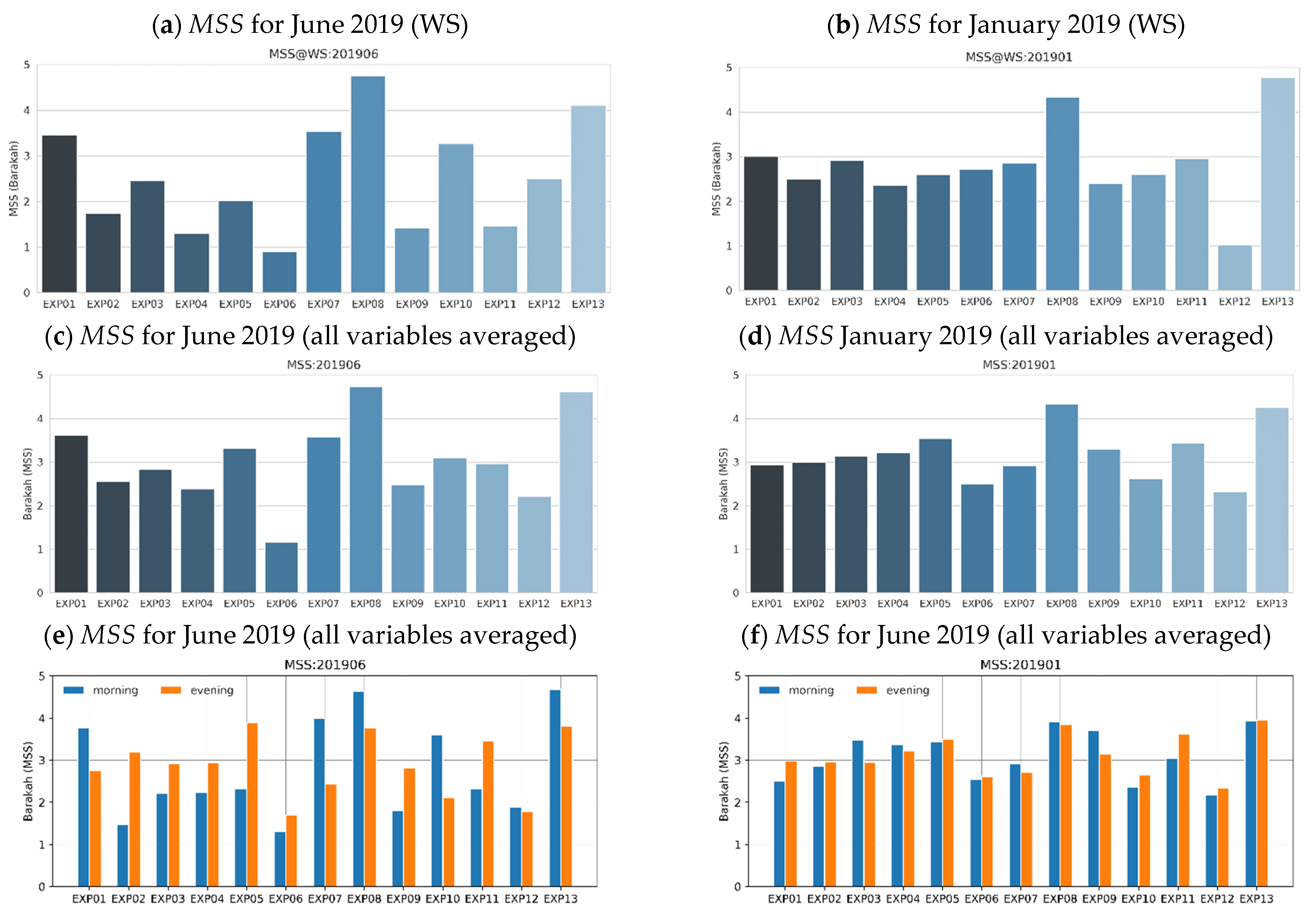
3.4.3. Model Simulations Ranking at Barakah
3.5. Statistical Model Evaluation at a Downwind Site
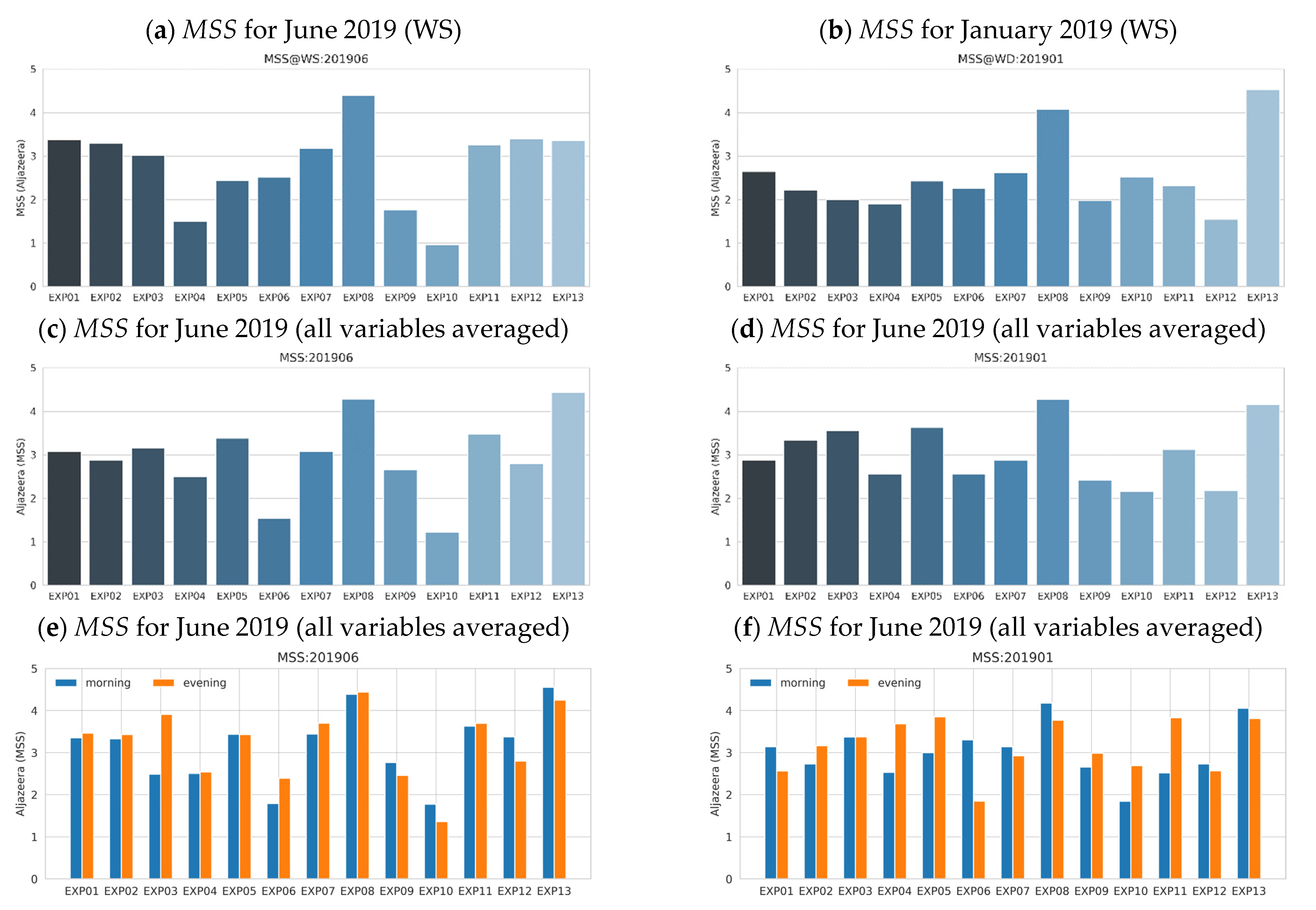
Model Simulations Ranking at Aljazeera
4. Summary and Conclusions
Author Contributions
Funding
Data Availability Statement
Acknowledgments
Conflicts of Interest
References
- Nesterov, O.; Temimi, M.; Fonseca, R.; Nelli, N.R.; Addad, Y.; Bosc, E.; Abida, R. Validation and Statistical Analysis of the Group for High Resolution Sea Surface Temperature Data in the Arabian Gulf. Oceanologia 2021, 63, 497–515. [Google Scholar] [CrossRef]
- Lelieveld, J.; Proestos, Y.; Hadjinicolaou, P.; Tanarhte, M.; Tyrlis, E.; Zittis, G. Strongly Increasing Heat Extremes in the Middle East and North Africa (MENA) in the 21st Century. Clim. Chang. 2016, 137, 245–260. [Google Scholar] [CrossRef] [Green Version]
- Feng, S.; Hu, Q.; Huang, W.; Ho, C.-H.; Li, R.; Tang, Z. Projected Climate Regime Shift under Future Global Warming from Multi-Model, Multi-Scenario CMIP5 Simulations. Glob. Planet. Chang. 2014, 112, 41–52. [Google Scholar] [CrossRef]
- Nelli, N.R.; Temimi, M.; Fonseca, R.M.; Weston, M.J.; Thota, M.S.; Valappil, V.K.; Branch, O.; Wizemann, H.D.; Wulfmeyer, V.; Wehbe, Y. Micrometeorological Measurements in an Arid Environment: Diurnal Characteristics and Surface Energy Balance Closure. Atmos. Res. 2020, 234, 104745. [Google Scholar] [CrossRef]
- Böer, B. An Introduction to the Climate of the United Arab Emirates. J. Arid Environ. 1997, 35, 3–16. [Google Scholar] [CrossRef]
- Francis, D.; Temimi, M.; Fonseca, R.; Nelli, N.R.; Abida, R.; Weston, M.; Whebe, Y. On the Analysis of a Summertime Convective Event in a Hyperarid Environment. Q. J. R. Meteorol. Soc. 2021, 147, 501–525. [Google Scholar] [CrossRef]
- Weston, M.J.; Temimi, M.; Burger, R.P.; Piketh, S.J. A Fog Climatology at Abu Dhabi International Airport. J. Appl. Meteorol. Climatol. 2021, 60, 223–236. [Google Scholar] [CrossRef]
- Weston, M.; Francis, D.; Nelli, N.; Fonseca, R.; Temimi, M.; Addad, Y. The First Characterisation of Fog Microphysics in the United Arab Emirates, an Arid Region on the Arabian Peninsula. Earth Space Sci. 2022, 9, 2021EA002032. [Google Scholar] [CrossRef]
- Fonseca, R.; Francis, D.; Weston, M.; Nelli, N.; Farah, S.; Wehbe, Y.; AlHosari, T.; Teixido, O.; Mohamed, R. Sensitivity of Summertime Convection to Aerosol Loading and Properties in the United Arab Emirates. Atmosphere 2021, 12, 1687. [Google Scholar] [CrossRef]
- Francis, D.; Chaboureau, J.-P.; Nelli, N.; Cuesta, J.; Alshamsi, N.; Temimi, M.; Pauluis, O.; Xue, L. Summertime Dust Storms over the Arabian Peninsula and Impacts on Radiation, Circulation, Cloud Development and Rain. Atmos. Res. 2021, 250, 105364. [Google Scholar] [CrossRef]
- Al Jallad, F.; Al Katheeri, E.; Al Omar, M. Levels of Particulate Matter in Western UAE Desert and Factors Affecting Their Distribution. Artif. Intell. Rev. 2013, 174, 111–122. [Google Scholar] [CrossRef] [Green Version]
- Abida, R.; Bocquet, M. Targeting of Observations for Accidental Atmospheric Release Monitoring. Atmos. Environ. 2009, 43, 6312–6327. [Google Scholar] [CrossRef]
- Abida, R.; Bocquet, M.; Vercauteren, N.; Isnard, O. Design of a Monitoring Network over France in Case of a Radiological Accidental Release. Atmos. Environ. 2008, 42, 5205–5219. [Google Scholar] [CrossRef]
- Korsakissok, I.; Mathieu, A.; Didier, D. Atmospheric Dispersion and Ground Deposition Induced by the Fukushima Nuclear Power Plant Accident: A Local-Scale Simulation and Sensitivity Study. Atmos. Environ. 2013, 70, 267–279. [Google Scholar] [CrossRef]
- Yoshikane, T.; Yoshimura, K. Dispersion Characteristics of Radioactive Materials Estimated by Wind Patterns. Sci. Rep. 2018, 8, 9926. [Google Scholar] [CrossRef]
- Yoshikane, T.; Yoshimura, K.; Chang, E.-C.; Saya, A.; Oki, T. Long-Distance Transport of Radioactive Plume by Nocturnal Local Winds. Sci. Rep. 2016, 6, 36584. [Google Scholar] [CrossRef] [Green Version]
- Aird, J.A.; Barthelmie, R.J.; Shepherd, T.J.; Pryor, S.C. WRF-Simulated Low-Level Jets over Iowa: Characterization and Sensitivity Studies. Wind Energy Sci. 2021, 6, 1015–1030. [Google Scholar] [CrossRef]
- Chaouch, N.; Temimi, M.; Weston, M.; Ghedira, H. Sensitivity of the Meteorological Model WRF-ARW to Planetary Boundary Layer Schemes during Fog Conditions in a Coastal Arid Region. Atmos. Res. 2017, 187, 106–127. [Google Scholar] [CrossRef]
- Fu, G.; Guo, J.; Xie, S.; Duan, Y.; Zhang, M. Analysis and High-Resolution Modeling of a Dense Sea Fog Event over the Yellow Sea. Atmos. Res. 2006, 81, 293–303. [Google Scholar] [CrossRef]
- Gao, S.; Lin, H.; Shen, B.; Fu, G. A Heavy Sea Fog Event over the Yellow Sea in March 2005: Analysis and Numerical Modeling. Adv. Atmos. Sci. 2007, 24, 65–81. [Google Scholar] [CrossRef]
- Hernández-Ceballos, M.A.; Adame, J.A.; Bolívar, J.P.; de la Morena, B.A. A Mesoscale Simulation of Coastal Circulation in the Guadalquivir Valley (Southwestern Iberian Peninsula) Using the WRF-ARW Model. Atmos. Res. 2013, 124, 1–20. [Google Scholar] [CrossRef]
- Steele, C.J.; Dorling, S.R.; von Glasow, R.; Bacon, J. Idealized WRF Model Sensitivity Simulations of Sea Breeze Types and Their Effects on Offshore Windfields. Atmos. Chem. Phys. 2013, 13, 443–461. [Google Scholar] [CrossRef] [Green Version]
- Tay, K.; Koh, T.-Y.; Skote, M. Characterizing Mesoscale Variability in Low-Level Jet Simulations for CBLAST-LOW 2001 Campaign. Meteorol. Atmos. Phys. 2021, 133, 163–179. [Google Scholar] [CrossRef]
- Yang, Y.; Hu, X.; Gao, S.; Wang, Y. Sensitivity of WRF Simulations with the YSU PBL Scheme to the Lowest Model Level Height for a Sea Fog Event over the Yellow Sea. Atmos. Res. 2019, 215, 253–267. [Google Scholar] [CrossRef]
- Powers, J.G.; Klemp, J.B.; Skamarock, W.C.; Davis, C.A.; Dudhia, J.; Gill, D.O.; Coen, J.L.; Gochis, D.J.; Ahmadov, R.; Peckham, S.E.; et al. The Weather Research and Forecasting Model: Overview, System Efforts, and Future Directions. Bull. Am. Meteorol. Soc. 2017, 98, 1717–1737. [Google Scholar] [CrossRef]
- Leelőssy, Á.; Molnár, F.; Izsák, F.; Havasi, Á.; Lagzi, I.; Mészáros, R. Dispersion Modeling of Air Pollutants in the Atmosphere: A Review. Cent. Eur. J. Geosci. 2014, 6, 257–278. [Google Scholar] [CrossRef]
- Storm, B.A.; Dudhia, J.; Basu, S.; Swift, A.J.; Giammanco, I.M. Evaluation of the Weather Research and Forecasting Model on Forecasting Low level Jets: Implications for Wind Energy. Wind Energy 2009, 12, 81–90. [Google Scholar] [CrossRef]
- Hu, X.; Nielsen-Gammon, J.W.; Zhang, F. Evaluation of Three Planetary Boundary Layer Schemes in the WRF Model. J. Appl. Meteorol. Climatol. 2010, 49, 1831–1844. [Google Scholar] [CrossRef] [Green Version]
- Kleczek, M.A.; Steeneveld, G.-J.; Holtslag, A.A.M. Evaluation of the Weather Research and Forecasting Mesoscale Model for GABLS3: Impact of Boundary-Layer Schemes, Boundary Conditions and Spin-Up. Bound. Layer Meteorol. 2014, 152, 213–243. [Google Scholar] [CrossRef]
- Rajeevan, M.; Kesarkar, A.P.; Thampi, S.B.; Rao, T.N.; Radhakrishna, B.P.; Rajasekhar, M. Sensitivity of WRF Cloud Microphysics to Simulations of a Severe Thunderstorm Event over Southeast India. Ann. Geophys. 2010, 28, 603–619. [Google Scholar] [CrossRef]
- Floors, R.; Vincent, C.L.; Gryning, S.-E.; Peña, A.; Batchvarova, E. The Wind Profile in the Coastal Boundary Layer: Wind Lidar Measurements and Numerical Modelling. Bound. Layer Meteorol. 2013, 147, 469–491. [Google Scholar] [CrossRef]
- Yang, Q.; Berg, L.K.; Pekour, M.S.; Fast, J.D.; Newsom, R.; Stoelinga, M.T.; Finley, C.A. Evaluation of WRF-Predicted Near-Hub-Height Winds and Ramp Events over a Pacific Northwest Site with Complex Terrain. J. Appl. Meteorol. Climatol. 2013, 52, 1753–1763. [Google Scholar] [CrossRef]
- Soni, M.; Payra, S.; Sinha, P.; Verma, S. A Performance Evaluation of WRF Model Using Different Physical Parameterization Scheme during Winter Season over a Semi-Arid Region, India. Inter. J. Earth Atmos. Sci. 2014, 1, 104–114. [Google Scholar]
- Carvalho, D.; Rocha, A.; Gómez-Gesteira, M.; Santos, C. A Sensitivity Study of the WRF Model in Wind Simulation for an Area of High Wind Energy. Environ. Model. Softw. 2012, 33, 23–34. [Google Scholar] [CrossRef] [Green Version]
- Dzebre, D.E.; Acheampong, A.A.; Ampofo, J.; Adaramola, M.S. A Sensitivity Study of Surface Wind Simulations over Coastal Ghana to Selected Time Control and Nudging Options in the Weather Research and Forecasting Model. Heliyon 2019, 5, e01385. [Google Scholar] [CrossRef] [Green Version]
- Chadee, X.T.; Seegobin, N.R.; Clarke, R.M. Optimizing the Weather Research and Forecasting (WRF) Model for Mapping the Near-Surface Wind Resources over the Southernmost Caribbean Islands of Trinidad and Tobago. Energies 2017, 10, 931. [Google Scholar] [CrossRef] [Green Version]
- Tyagi, B.; Magliulo, V.; Finardi, S.; Gasbarra, D.; Carlucci, P.; Toscano, P.; Zaldei, A.; Riccio, A.; Calori, G.; D’Allura, A.; et al. Performance Analysis of Planetary Boundary Layer Parameterization Schemes in WRF Modeling Set Up over Southern Italy. Atmosphere 2018, 9, 272. [Google Scholar] [CrossRef] [Green Version]
- Boadh, R.; Satyanarayana, A.N.V.; Rama Krishna, T.V.B.P.S.; Madala, S. Sensitivity of PBL Schemes of the WRF-ARW Model in Simulating the Boundary Layer Flow Parameters for Their Application to Air Pollution Dispersion Modeling over a Tropical Station. Atmósfera 2016, 29, 61–81. [Google Scholar] [CrossRef] [Green Version]
- Taraphdar, S.; Pauluis, O.M.; Xue, L.; Liu, C.; Rasmussen, R.; Ajayamohan, R.S.; Tessendorf, S.; Jing, X.; Chen, S.; Grabowski, W.W. WRF Gray-Zone Simulations of Precipitation Over the Middle-East and the UAE: Impacts of Physical Parameterizations and Resolution. J. Geophys. Res. Atmos. 2021, 126, e2021JD034648. [Google Scholar] [CrossRef]
- Yu, N.; Barthe, C.; Plu, M. Evaluating Intense Precipitation in High-Resolution Numerical Model over a Tropical Island: Impact of Model Horizontal Resolution. Nat. Hazards Earth Syst. Sci. Discuss 2014, 2, 999–1032. [Google Scholar] [CrossRef]
- Pokhrel, R.; Lee, H. Estimation of the Effective Zone of Sea/Land Breeze in a Coastal Area. Atmos. Pollut. Res. 2011, 2, 106–115. [Google Scholar] [CrossRef] [Green Version]
- Skamarock, C.; Klemp, B.; Dudhia, J.; Gill, O.; Barker, D.M.; Duda, G.; Huang, X.; Wang, W.; Powers, G. A Description of the Advanced Research WRF Version 3; University Corporation for Atmospheric Research: Boulder, CO, USA, 2008. [Google Scholar] [CrossRef]
- Di, Z.; Gong, W.; Gan, Y.; Shen, C.; Duan, Q. Combinatorial Optimization for WRF Physical Parameterization Schemes: A Case Study of Three-Day Typhoon Simulations over the Northwest Pacific Ocean. Atmosphere 2019, 10, 233. [Google Scholar] [CrossRef] [Green Version]
- Krieger, J.R.; Zhang, J.; Atkinson, D.E.; Zhang, X. Sensitivity of WRF Model Forecasts to Different Physical Parameterizations in the Beaufort Sea Region. In Proceedings of the 8th Conference on Coastal Atmospheric and Oceanic Prediction and Processes, San Diego, CA, USA, 10–15 January 2009. [Google Scholar]
- Zhang, Y.; Sartelet, K.; Zhu, S.; Wang, W.; Wu, S.-Y.; Zhang, X.; Wang, K.; Tran, P.; Seigneur, C.; Wang, Z.-F. Application of WRF/Chem-MADRID and WRF/Polyphemus in Europe—Part 2: Evaluation of Chemical Concentrations and Sensitivity Simulations. Atmos. Chem. Phys. 2013, 13, 6845–6875. [Google Scholar] [CrossRef] [Green Version]
- Nakanishi, M.; Niino, H. An Improved Mellor–Yamada Level-3 Model: Its Numerical Stability and Application to a Regional Prediction of Advection Fog. Bound. Layer Meteorol. 2006, 119, 397–407. [Google Scholar] [CrossRef]
- Mellor, G.L.; Yamada, T. Development of a Turbulence Closure Model for Geophysical Fluid Problems. Rev. Geophys. 1982, 20, 851–875. [Google Scholar] [CrossRef] [Green Version]
- Sukoriansky, S.; Galperin, B.; Perov, V. A Quasi-Normal Scale Elimination Model of Turbulence and Its Application to Stably Stratified Flows. Nonlinear Process. Geophys. 2006, 13, 9–22. [Google Scholar] [CrossRef]
- Hong, S.-Y.; Noh, Y.; Dudhia, J. A New Vertical Diffusion Package with an Explicit Treatment of Entrainment Processes. Mon. Weather Rev. 2006, 134, 2318–2341. [Google Scholar] [CrossRef] [Green Version]
- Pleim, J.E. A Combined Local and Nonlocal Closure Model for the Atmospheric Boundary Layer. Part I: Model Description and Testing. J. Appl. Meteorol. Climatol. 2007, 46, 1383–1395. [Google Scholar] [CrossRef]
- Dudhia, J. Numerical Study of Convection Observed during the Winter Monsoon Experiment Using a Mesoscale Two-Dimensional Model. J. Atmos. Sci. 1989, 46, 3077–3107. [Google Scholar] [CrossRef]
- Iacono, M.J.; Delamere, J.S.; Mlawer, E.J.; Shephard, M.W.; Clough, S.A.; Collins, W.D. Radiative Forcing by Longlived Greenhouse Gases: Calculations with the AER Radiative Transfer Models. J. Geophys. Res. 2008, 113, D13. [Google Scholar] [CrossRef]
- Mlawer, E.J.; Taubman, S.J.; Brown, P.D.; Iacono, M.J.; Clough, S.A. Radiative Transfer for Inhomogeneous Atmospheres: RRTM, a Validated Correlated-k Model for the Longwave. J. Geophys. Res. 1997, 102, 16663–16682. [Google Scholar] [CrossRef] [Green Version]
- Jiménez, P.A.; Dudhia, J.; Navarro, J. A Revised Scheme for the WRF Surface Layer Formulation. Mon. Weather Rev. 2012, 140, 898–918. [Google Scholar] [CrossRef] [Green Version]
- Skamarock, W.C. Evaluating Mesoscale NWP Models Using Kinetic Energy Spectra. Mon. Weather Rev. 2004, 132, 3019–3032. [Google Scholar] [CrossRef]
- Abida, R.; Attié, J.-L.; el Amraoui, L.; Ricaud, P.; Lahoz, W.; Eskes, H.; Segers, A.; Curier, L.; de Haan, J.; Kujanpää, J.; et al. Impact of Spaceborne Carbon Monoxide Observations from the S-5P Platform on tropospheric Composition Analyses and Forecasts. Atmos. Chem. Phys. 2017, 17, 1081–1103. [Google Scholar] [CrossRef] [Green Version]
- Surussavadee, C. Evaluation of WRF Near-Surface Wind Simulations in Tropics Employing Different Planetary Boundary Layer Schemes. In Proceedings of the 2017 8th International Renewable Energy Congress (IREC), Amman, Jordan, 21–23 March 2017; pp. 1–4. [Google Scholar] [CrossRef]
- Agostinelli, C.; Lund, U. R Package:Circular Statistics (Version 0.4-93). 2017. Available online: https://R-Forge.r-Project.Org/Projects/Circular/ (accessed on 15 May 2022).
- Gbode, I.E.; Dudhia, J.; Ogunjobi, K.O.; Ajayi, V.O. Sensitivity of Different Physics Schemes in the WRF Model during a West African Monsoon Regime. Theor. Appl. Climatol. 2018, 136, 733–751. [Google Scholar] [CrossRef] [Green Version]
- Charnock, H. Wind Stress on a Water Surface. Q. J. R. Meteorol. Soc. 1955, 81, 639–640. [Google Scholar] [CrossRef]
- Lee, J.A.; Hacker, J.P.; Monache, L.D.; Kosović, B.; Clifton, A.; Vandenberghe, F.; Rodrigo, J.S. Improving Wind Predictions in the Marine Atmospheric Boundary Layer Through Parameter Estimation in a Single Column Model. Mon. Weather Rev. 2017, 145, 5–24. [Google Scholar] [CrossRef]
- Fonseca, R.; Temimi, M.; Thota, M.S.; Nelli, N.R.; Weston, M.J.; Suzuki, K.; Uchida, J.; Kumar, K.N.; Branch, O.; Wehbe, Y.; et al. On the Analysis of the Performance of WRF and NICAM in a Hyperarid Environment. Weather Forecast. 2020, 35, 891–919. [Google Scholar] [CrossRef] [Green Version]
- Fonseca, R.; Francis, D.; Nelli, N.; Thota, M. Climatology of the Heat Low and the Intertropical Discontinuity in the Arabian Peninsula. Int. J. Climatol. 2022, 42, 1092–1117. [Google Scholar] [CrossRef]
- Dumka, U.C.; Kaskaoutis, D.G.; Francis, D.; Chaboureau, J.-P.; Rashki, A.; Tiwari, S.; Singh, S.; Liakakou, E.; Mihalopoulos, N. The Role of the Intertropical Discontinuity Region and the Heat Low in Dust Emission and Transport Over the Thar Desert, India: A Premonsoon Case Study. J. Geophys. Res. Atmos. 2019, 124, 13197–13219. [Google Scholar] [CrossRef]
- Nelli, N.; Fissehaye, S.; Francis, D.; Fonseca, R.; Temimi, M.; Weston, M.; Abida, R.; Nesterov, O. Characteristics of Atmospheric Aerosols over the UAE Inferred from CALIPSO and Sun Photometer Aerosol Optical Depth. Earth Space Sci. Open Arch. 2020, 37, e2020EA001360. [Google Scholar] [CrossRef]
- Branch, O.; Schwitalla, T.; Temimi, M.; Fonseca, R.; Nelli, N.; Weston, M.; Milovac, J.; Wulfmeyer, V. Seasonal and Diurnal Performance of Daily Forecasts with WRF V3.8.1 over the United Arab Emirates. Geosci. Model Dev. 2021, 14, 1615–1637. [Google Scholar] [CrossRef]
- Borge, R.; Alexandrov, V.N.; del Vas, J.J.; Lumbreras, J.; Rodríguez, E. A Comprehensive Sensitivity Analysis of the WRF Model for Air Quality Applications over the Iberian Peninsula. Atmos. Environ. 2008, 42, 8560–8574. [Google Scholar] [CrossRef]
- Kwun, J.; Kim, Y.-K.; Seo, J.-W.; Jeong, J.-H.; You, S.H. Sensitivity of MM5 and WRF Mesoscale Model Predictions of Surface Winds in a Typhoon to Planetary Boundary Layer Parameterizations. Nat. Hazards 2009, 51, 63–77. [Google Scholar] [CrossRef]
- Ruiz, J.; Saulo, C.; Nogués-Paegle, J. WRF Model Sensitivity to Choice of Parameterization over South America: Validation against Surface Variables. Mon. Weather Rev. 2010, 138, 3342–3355. [Google Scholar] [CrossRef]
- García-Díez, M.; Fernández, J.; Fita, L.; Yagüe, C. Seasonal Dependence of WRF Model Biases and Sensitivity to PBL Schemes over Europe. Q. J. R. Meteorol. Soc. 2013, 139, 501–514. [Google Scholar] [CrossRef] [Green Version]
- Weston, M.; Chaouch, N.; Valappil, V.; Temimi, M.; Ek, M.; Zheng, W. Assessment of the Sensitivity to the Thermal Roughness Length in Noah and Noah-MP Land Surface Model Using WRF in an Arid Region. Pure Appl. Geophys. 2019, 176, 2121–2137. [Google Scholar] [CrossRef]


| Station ID | Station Name | Latitude | Longitude | Elevation (m) | Station Type | Distance from BNPP | Cardinal Direction from BNPP | Provider |
|---|---|---|---|---|---|---|---|---|
| 1 | Qarnen | 24.9416 | 52.8497 | 32 | offshore | 125 | NE | NCM |
| 2 | Dalma | 24.4908 | 52.2913 | 25 | offshore | 58 | NNE | NCM |
| 3 | SirBaniYas | 24.3169 | 52.5977 | 14 | offshore | 54 | NE | NCM |
| 4 | Yasat | 24.1722 | 51.9883 | 12 | offshore | 34 | NW | NCM |
| 5 | Nawah Tower | 23.9599 | 52.2387 | 4 | nearshore | 1.2 | ESE | NCM |
| 6 | Barakah | 23.9552 | 52.2663 | 5 | nearshore | 3.8 | ESE | Nawah |
| 7 | AlRuwais | 24.0933 | 52.6227 | 32 | nearshore | 42 | ENE | NCM |
| 8 | AlGheweifat | 24.1211 | 51.6269 | 69 | nearshore | 64 | WNW | NCM |
| 9 | Aljazeera | 23.2911 | 52.2888 | 70 | inland | 75 | S | NCM |
| 10 | Owtaid | 23.3955 | 53.1027 | 180 | inland | 109 | SE | NCM |
| 11 | Mukhariz | 22.9347 | 52.8777 | 145 | inland | 132 | SSE | NCM |
| 12 | MadinatZayed | 23.6816 | 53.6986 | 118 | inland | 152 | ESE | NCM |
| Non-Hydrostatic Model | Advanced Research WRF v4.2 | ||
|---|---|---|---|
| Driving data | NCEP GFS at 0.25° spatial and 6-hourly temporal resolution, and 32 pressure vertical levels. Time-varying analyzed GFS SST. Held constant during the model integration time period | ||
| Land use data | 20-category MODIS at 30 arc-seconds | ||
| Geographical projection scheme | Mercator | ||
| Horizontal grid system | Arakawa-C grid | ||
| Horizontal resolution (km) | 25 | 5 | 1 |
| Domain size (grid-points) | 61 × 91 | 131 × 201 | 311 × 311 |
| Vertical resolution | 45 terrain-following sigma-pressure vertical levels | ||
| Integration time step | 120 s | ||
| Time integration scheme | 3rd order Runge-Kutta scheme | ||
| Spatial differencing scheme | 6th order center differencing | ||
| Spin-up time period | 12 h | ||
| Integration time period | 36 h | ||
| Simulation ID | Microphysics | LW RAD | SW RAD | Surface Layer | Land Surface | PBL | Cumulus |
|---|---|---|---|---|---|---|---|
| EXP01 | WSM 3-class | RRTM | Dudhia | Revised MM5 | Thermal Diffusion | YSU | BMJ |
| EXP02 | Thompson graupel | RRTMG | RRTMG | MYNN | Unified Noah Model | MYNN 2.5 | BMJ |
| EXP03 | Thompson graupel | RRTMG | RRTMG | Revised MM5 | Unified Noah Model | YSU | Kain-Fritsch |
| EXP04 | Thompson graupel | RRTM | RRTMG | QNSE | Unified Noah Model | QNSE-EDMF | Kain-Fritsch |
| EXP05 | Thompson graupel | RRTM | RRTMG | Monin-Obukhov | Unified Noah Model | MYJ | Kain-Fritsch |
| EXP06 | Thompson graupel | RRTM | RRTMG | MYNN | Unified Noah Model | MYNN3 | Kain-Fritsch |
| EXP07 | Thompson graupel | RRTM | RRTMG | Revised MM5 | Thermal Diffusion | YSU | Kain-Fritsch |
| EXP08 | WSM 3-class | RRTM | RRTMG | Revised MM5 | Thermal Diffusion | YSU | Kain-Fritsch |
| EXP09 | Perdue Line | RRTM | Dudhia | QNSE | Unified Noah Model | QNSE-EDMF | Kain-Fritsch |
| EXP10 | Perdue Line | RRTM | Dudhia | QNSE | Thermal Diffusion | QNSE-EDMF | Kain-Fritsch |
| EXP11 | Thompson graupel | RRTM | RRTMG | Pleim Xiu | Unified Noah Model | ACM2 | Kain-Fritsch |
| EXP12 | Thompson graupel | RRTM | RTTMG | Revised MM5 | Noah-MP Model | YSU | Kain-Fritsch |
| EXP13 | WSM 3-class | RRTM | RRTMG | Revised MM5 | Thermal Diffusion | YSU with topo_wind option enabled | Kain-Fritsch |
| EXP01 | EXP02 | EXP03 | EXP04 | EXP05 | EXP06 | EXP07 | EXP08 | EXP09 | EXP10 | EXP11 | EXP12 | EXP13 | |
|---|---|---|---|---|---|---|---|---|---|---|---|---|---|
| 2 m Air Temperature (°C) | |||||||||||||
| ρ | 0.954 | 0.883 | 0.895 | 0.865 | 0.871 | 0.861 | 0.947 | 0.964 | 0.878 | 0.948 | 0.878 | 0.813 | 0.962 |
| MB | −0.836 | −1.185 | −1.037 | −1.730 | −1.076 | −2.113 | −0.816 | −0.821 | −1.754 | −1.597 | −0.935 | −1.255 | −0.802 |
| MAE | 1.363 | 1.988 | 1.973 | 2.339 | 2.096 | 2.629 | 1.396 | 1.208 | 2.273 | 1.880 | 1.991 | 2.519 | 1.219 |
| RMSE | 1.723 | 2.544 | 2.428 | 2.952 | 2.592 | 3.243 | 1.759 | 1.545 | 2.880 | 2.236 | 2.472 | 3.057 | 1.575 |
| STDE | 1.507 | 2.251 | 2.196 | 2.392 | 2.358 | 2.460 | 1.559 | 1.309 | 2.284 | 1.564 | 2.289 | 2.788 | 1.355 |
| 2 m Relative Humidity (%) | |||||||||||||
| ρ | 0.854 | 0.848 | 0.854 | 0.836 | 0.870 | 0.832 | 0.863 | 0.887 | 0.843 | 0.837 | 0.858 | 0.828 | 0.890 |
| MB | 11.846 | 13.721 | 14.068 | 15.302 | 11.938 | 20.411 | 12.330 | 10.917 | 14.987 | 14.771 | 10.739 | 15.011 | 10.444 |
| MAE | 13.481 | 14.755 | 15.158 | 16.658 | 13.309 | 20.690 | 13.512 | 11.942 | 16.266 | 15.829 | 12.613 | 16.398 | 11.730 |
| RMSE | 17.424 | 17.712 | 17.994 | 19.614 | 15.952 | 23.614 | 17.301 | 15.276 | 19.249 | 19.578 | 15.668 | 19.444 | 15.040 |
| STDE | 12.778 | 11.201 | 11.218 | 12.271 | 10.580 | 11.875 | 12.136 | 10.684 | 12.080 | 12.850 | 11.409 | 12.360 | 10.823 |
| 10 m wind speed (m/s) | |||||||||||||
| ρ | 0.891 | 0.829 | 0.860 | 0.836 | 0.854 | 0.820 | 0.888 | 0.916 | 0.836 | 0.869 | 0.836 | 0.850 | 0.906 |
| MB | 0.207 | −0.208 | −0.212 | −0.375 | −0.298 | −0.347 | 0.162 | 0.09 | −0.347 | −0.031 | −0.319 | 0.143 | −0.17 |
| MAE | 0.840 | 1.033 | 0.960 | 1.024 | 0.974 | 1.097 | 0.844 | 0.721 | 1.016 | 0.915 | 1.033 | 0.963 | 0.771 |
| RMSE | 1.074 | 1.313 | 1.208 | 1.329 | 1.246 | 1.380 | 1.078 | 0.935 | 1.321 | 1.164 | 1.315 | 1.231 | 0.997 |
| STDE | 1.054 | 1.297 | 1.190 | 1.275 | 1.209 | 1.336 | 1.066 | 0.931 | 1.274 | 1.164 | 1.276 | 1.222 | 0.983 |
| 10 m wind direction (°) | |||||||||||||
| ρ | 0.732 | 0.715 | 0.723 | 0.725 | 0.731 | 0.720 | 0.744 | 0.781 | 0.706 | 0.704 | 0.732 | 0.715 | 0.790 |
| MB | 10.028 | 11.989 | 11.080 | 11.983 | 10.522 | 10.909 | 11.483 | 9.624 | 10.253 | 10.581 | 13.394 | 12.331 | 9.787 |
| MAE | 30.293 | 31.569 | 31.459 | 27.635 | 27.559 | 33.349 | 30.198 | 26.950 | 28.781 | 28.858 | 28.568 | 31.763 | 26.379 |
| RMSE | 47.542 | 49.677 | 49.508 | 43.151 | 44.245 | 53.065 | 47.803 | 44.141 | 44.837 | 46.331 | 45.050 | 48.756 | 43.173 |
| STDE | 46.472 | 48.209 | 48.252 | 41.454 | 42.976 | 51.932 | 46.403 | 43.078 | 43.649 | 45.106 | 43.013 | 47.171 | 42.049 |
| EXP01 | EXP02 | EXP03 | EXP04 | EXP05 | EXP06 | EXP07 | EXP08 | EXP09 | EXP10 | EXP11 | EXP12 | EXP13 | |
|---|---|---|---|---|---|---|---|---|---|---|---|---|---|
| 2 m Air Temperature (°C) | |||||||||||||
| ρ | 0.952 | 0.951 | 0.952 | 0.945 | 0.959 | 0.960 | 0.958 | 0.965 | 0.944 | 0.940 | 0.952 | 0.943 | 0.962 |
| MB | 0.138 | 0.488 | 0.680 | 0.444 | 0.501 | -0.250 | 0.443 | 0.304 | 0.217 | -0.120 | 0.836 | 0.977 | 0.179 |
| MAE | 1.050 | 1.140 | 1.193 | 1.247 | 1.042 | 0.942 | 1.084 | 0.949 | 1.202 | 1.211 | 1.315 | 1.475 | 1.003 |
| RMSE | 1.418 | 1.452 | 1.503 | 1.521 | 1.344 | 1.264 | 1.401 | 1.240 | 1.484 | 1.557 | 1.595 | 1.798 | 1.296 |
| STDE | 1.411 | 1.367 | 1.337 | 1.455 | 1.247 | 1.239 | 1.328 | 1.202 | 1.468 | 1.552 | 1.359 | 1.510 | 1.284 |
| 2 m Relative Humidity (%) | |||||||||||||
| ρ | 0.896 | 0.890 | 0.901 | 0.908 | 0.904 | 0.883 | 0.901 | 0.919 | 0.906 | 0.893 | 0.907 | 0.902 | 0.913 |
| MB | 7.133 | 1.545 | 0.997 | 3.772 | 3.302 | 7.140 | 6.295 | 5.929 | 3.539 | 10.083 | 0.487 | 0.644 | 6.230 |
| MAE | 8.796 | 6.051 | 5.543 | 6.371 | 6.537 | 9.435 | 8.154 | 7.433 | 6.372 | 10.797 | 5.501 | 5.320 | 7.853 |
| RMSE | 11.201 | 8.486 | 7.775 | 8.757 | 8.470 | 11.441 | 10.418 | 9.498 | 8.637 | 13.207 | 7.595 | 7.538 | 10.014 |
| STDE | 8.636 | 8.344 | 7.711 | 7.903 | 7.801 | 8.940 | 8.302 | 7.419 | 7.879 | 8.530 | 7.579 | 7.510 | 7.840 |
| 10 m wind speed (m/s) | |||||||||||||
| ρ | 0.840 | 0.822 | 0.829 | 0.823 | 0.831 | 0.823 | 0.839 | 0.867 | 0.815 | 0.819 | 0.823 | 0.822 | 0.863 |
| MB | 0.353 | 0.289 | 0.255 | 0.248 | 0.335 | 0.210 | 0.395 | 0.283 | 0.177 | 0.144 | 0.180 | 0.674 | 0.003 |
| MAE | 0.941 | 0.965 | 0.939 | 0.994 | 0.974 | 0.952 | 0.950 | 0.834 | 0.975 | 0.970 | 0.928 | 1.127 | 0.813 |
| RMSE | 1.254 | 1.309 | 1.268 | 1.318 | 1.292 | 1.292 | 1.269 | 1.135 | 1.326 | 1.305 | 1.274 | 1.439 | 1.117 |
| STDE | 1.203 | 1.277 | 1.243 | 1.294 | 1.248 | 1.275 | 1.206 | 1.099 | 1.314 | 1.297 | 1.261 | 1.271 | 1.117 |
| 10 m wind direction (°) | |||||||||||||
| ρ | 0.862 | 0.863 | 0.868 | 0.879 | 0.886 | 0.841 | 0.867 | 0.894 | 0.880 | 0.876 | 0.891 | 0.850 | 0.896 |
| MB | 14.298 | 15.017 | 16.288 | 15.853 | 16.461 | 17.127 | 15.373 | 12.789 | 16.075 | 15.516 | 14.939 | 15.553 | 12.878 |
| MAE | 25.197 | 25.892 | 25.639 | 23.810 | 24.240 | 27.830 | 25.444 | 22.559 | 24.211 | 24.210 | 23.762 | 26.116 | 22.167 |
| RMSE | 39.332 | 40.075 | 40.480 | 36.092 | 36.415 | 42.514 | 39.745 | 36.067 | 36.090 | 36.097 | 37.143 | 39.670 | 36.129 |
| STDE | 36.641 | 37.155 | 37.058 | 32.424 | 32.483 | 38.912 | 36.651 | 33.724 | 32.313 | 32.593 | 34.006 | 36.494 | 33.756 |
| EXP01 | EXP02 | EXP03 | EXP04 | EXP05 | EXP06 | EXP07 | EXP08 | EXP09 | EXP10 | EXP11 | EXP12 | EXP13 | |
|---|---|---|---|---|---|---|---|---|---|---|---|---|---|
| 2 m Air Temperature (K) | |||||||||||||
| ρ | 0.986 | 0.982 | 0.985 | 0.977 | 0.977 | 0.977 | 0.986 | 0.990 | 0.978 | 0.980 | 0.980 | 0.981 | 0.992 |
| MB | −0.785 | −0.724 | −0.703 | −0.978 | −0.567 | −1.426 | −0.739 | −0.738 | −0.981 | −1.687 | −0.443 | −0.497 | −0.643 |
| MAE | 1.129 | 1.116 | 1.037 | 1.355 | 1.147 | 1.604 | 1.039 | 0.957 | 1.337 | 1.845 | 1.040 | 1.104 | 0.863 |
| RMSE | 1.424 | 1.483 | 1.323 | 1.740 | 1.516 | 1.987 | 1.342 | 1.212 | 1.708 | 2.172 | 1.398 | 1.464 | 1.115 |
| STDE | 1.189 | 1.294 | 1.121 | 1.439 | 1.406 | 1.384 | 1.121 | 0.961 | 1.398 | 1.369 | 1.326 | 1.377 | 0.911 |
| 2 m Relative Humidity (%) | |||||||||||||
| ρ | 0.946 | 0.943 | 0.938 | 0.928 | 0.934 | 0.922 | 0.944 | 0.956 | 0.936 | 0.920 | 0.939 | 0.936 | 0.961 |
| MB | 7.549 | 6.990 | 6.624 | 6.148 | 4.898 | 11.595 | 7.867 | 7.167 | 5.718 | 11.476 | 5.060 | 7.050 | 6.167 |
| MAE | 8.175 | 7.817 | 7.694 | 7.589 | 6.536 | 11.820 | 8.418 | 7.598 | 7.324 | 11.929 | 6.556 | 8.131 | 6.737 |
| RMSE | 11.423 | 11.026 | 10.666 | 10.945 | 9.681 | 15.644 | 11.456 | 10.266 | 10.522 | 15.216 | 9.611 | 11.317 | 9.297 |
| STDE | 8.573 | 8.527 | 8.360 | 9.055 | 8.351 | 10.502 | 8.329 | 7.350 | 8.833 | 9.991 | 8.171 | 8.853 | 6.956 |
| 10 m wind speed (m/s) | |||||||||||||
| ρ | 0.89 | 0.887 | 0.888 | 0.858 | 0.877 | 0.885 | 0.890 | 0.918 | 0.859 | 0.864 | 0.890 | 0.875 | 0.914 |
| MB | −0.408 | −0.336 | −0.429 | −0.648 | −0.553 | −0.510 | −0.458 | −0.469 | −0.560 | −0.852 | −0.420 | 0.058 | −0.727 |
| MAE | 1.084 | 1.103 | 1.128 | 1.256 | 1.162 | 1.177 | 1.105 | 0.977 | 1.238 | 1.344 | 1.103 | 1.102 | 1.101 |
| RMSE | 1.426 | 1.439 | 1.469 | 1.673 | 1.551 | 1.534 | 1.449 | 1.290 | 1.634 | 1.735 | 1.438 | 1.461 | 1.427 |
| STDE | 1.366 | 1.401 | 1.405 | 1.542 | 1.449 | 1.446 | 1.374 | 1.202 | 1.535 | 1.511 | 1.376 | 1.460 | 1.228 |
| 10 m wind direction (°) | |||||||||||||
| ρ | 0.715 | 0.707 | 0.726 | 0.698 | 0.757 | 0.707 | 0.711 | 0.787 | 0.685 | 0.662 | 0.724 | 0.687 | 0.799 |
| MB | 12.528 | 13.661 | 11.115 | 9.316 | 10.763 | 12.385 | 12.741 | 10.266 | 8.971 | 9.181 | 11.716 | 13.459 | 8.492 |
| MAE | 25.759 | 26.374 | 26.231 | 25.998 | 24.109 | 26.999 | 25.499 | 22.068 | 26.306 | 26.774 | 24.981 | 27.048 | 20.942 |
| RMSE | 39.262 | 40.873 | 40.187 | 39.104 | 35.788 | 41.818 | 39.668 | 34.604 | 39.153 | 41.015 | 38.138 | 41.570 | 33.733 |
| STDE | 37.210 | 38.522 | 38.619 | 37.978 | 34.131 | 39.942 | 37.566 | 33.046 | 38.111 | 39.975 | 36.294 | 39.331 | 32.646 |
| EXP01 | EXP02 | EXP03 | EXP04 | EXP05 | EXP06 | EXP07 | EXP08 | EXP09 | EXP10 | EXP11 | EXP12 | EXP13 | |
|---|---|---|---|---|---|---|---|---|---|---|---|---|---|
| 2 m Air Temperature (K) | |||||||||||||
| ρ | 0.981 | 0.978 | 0.984 | 0.973 | 0.983 | 0.979 | 0.982 | 0.986 | 0.970 | 0.976 | 0.976 | 0.978 | 0.986 |
| MB | 0.482 | 0.263 | 0.433 | 0.117 | 0.417 | −0.170 | 0.771 | 0.604 | −0.183 | 0.032 | 0.525 | 0.606 | 0.543 |
| MAE | 0.947 | 0.968 | 0.887 | 1.091 | 0.890 | 0.920 | 1.082 | 0.901 | 1.101 | 0.978 | 1.112 | 1.151 | 0.892 |
| RMSE | 1.223 | 1.244 | 1.119 | 1.343 | 1.145 | 1.179 | 1.330 | 1.129 | 1.409 | 1.262 | 1.375 | 1.409 | 1.125 |
| STDE | 1.124 | 1.216 | 1.032 | 1.338 | 1.067 | 1.166 | 1.084 | 0.953 | 1.397 | 1.261 | 1.271 | 1.272 | 0.985 |
| 2 m Relative Humidity (%) | |||||||||||||
| ρ | 0.915 | 0.924 | 0.929 | 0.920 | 0.921 | 0.893 | 0.920 | 0.935 | 0.923 | 0.913 | 0.927 | 0.926 | 0.935 |
| MB | 5.127 | 1.700 | 1.046 | 3.186 | 2.605 | 7.138 | 4.422 | 4.098 | 3.541 | 9.846 | 1.180 | 2.158 | 3.991 |
| MAE | 7.416 | 5.922 | 5.355 | 6.363 | 6.410 | 9.136 | 7.026 | 6.321 | 6.418 | 10.609 | 5.821 | 6.068 | 6.320 |
| RMSE | 10.221 | 8.193 | 7.629 | 8.898 | 8.631 | 12.429 | 9.651 | 8.703 | 8.802 | 13.115 | 7.893 | 8.581 | 8.601 |
| STDE | 8.842 | 8.014 | 7.557 | 8.308 | 8.228 | 10.176 | 8.579 | 7.677 | 8.058 | 8.663 | 7.804 | 8.305 | 7.618 |
| 10 m wind speed (m/s) | |||||||||||||
| ρ | 0.841 | 0.868 | 0.857 | 0.845 | 0.876 | 0.854 | 0.853 | 0.885 | 0.845 | 0.844 | 0.870 | 0.853 | 0.886 |
| MB | −0.090 | −0.045 | −0.032 | −0.291 | −0.155 | −0.054 | −0.026 | −0.092 | −0.338 | −0.438 | −0.086 | 0.377 | −0.332 |
| MAE | 0.878 | 0.891 | 0.867 | 0.879 | 0.818 | 0.944 | 0.853 | 0.768 | 0.891 | 0.913 | 0.832 | 0.960 | 0.801 |
| RMSE | 1.242 | 1.161 | 1.200 | 1.260 | 1.125 | 1.215 | 1.196 | 1.080 | 1.271 | 1.302 | 1.151 | 1.253 | 1.133 |
| STDE | 1.239 | 1.160 | 1.200 | 1.226 | 1.114 | 1.214 | 1.196 | 1.076 | 1.225 | 1.226 | 1.148 | 1.195 | 1.083 |
| 10 m wind direction (°) | |||||||||||||
| ρ | 0.871 | 0.870 | 0.867 | 0.833 | 0.864 | 0.878 | 0.875 | 0.906 | 0.837 | 0.847 | 0.865 | 0.846 | 0.915 |
| MB | 13.465 | 13.323 | 12.718 | 8.788 | 11.687 | 15.240 | 13.305 | 11.929 | 7.900 | 8.980 | 11.983 | 14.440 | 10.784 |
| MAE | 21.983 | 22.759 | 23.041 | 23.013 | 22.087 | 23.335 | 22.079 | 19.218 | 23.329 | 22.023 | 22.068 | 23.988 | 18.370 |
| RMSE | 32.489 | 33.940 | 34.995 | 37.305 | 34.217 | 32.511 | 32.595 | 28.930 | 37.167 | 35.095 | 34.573 | 35.415 | 28.104 |
| STDE | 29.568 | 31.216 | 32.602 | 36.255 | 32.159 | 28.718 | 29.756 | 26.356 | 36.318 | 33.927 | 32.430 | 32.337 | 25.952 |
Publisher’s Note: MDPI stays neutral with regard to jurisdictional claims in published maps and institutional affiliations. |
© 2022 by the authors. Licensee MDPI, Basel, Switzerland. This article is an open access article distributed under the terms and conditions of the Creative Commons Attribution (CC BY) license (https://creativecommons.org/licenses/by/4.0/).
Share and Cite
Abida, R.; Addad, Y.; Francis, D.; Temimi, M.; Nelli, N.; Fonseca, R.; Nesterov, O.; Bosc, E. Evaluation of the Performance of the WRF Model in a Hyper-Arid Environment: A Sensitivity Study. Atmosphere 2022, 13, 985. https://doi.org/10.3390/atmos13060985
Abida R, Addad Y, Francis D, Temimi M, Nelli N, Fonseca R, Nesterov O, Bosc E. Evaluation of the Performance of the WRF Model in a Hyper-Arid Environment: A Sensitivity Study. Atmosphere. 2022; 13(6):985. https://doi.org/10.3390/atmos13060985
Chicago/Turabian StyleAbida, Rachid, Yacine Addad, Diana Francis, Marouane Temimi, Narendra Nelli, Ricardo Fonseca, Oleksandr Nesterov, and Emmanuel Bosc. 2022. "Evaluation of the Performance of the WRF Model in a Hyper-Arid Environment: A Sensitivity Study" Atmosphere 13, no. 6: 985. https://doi.org/10.3390/atmos13060985