Article

Development of a CNN+LSTM Hybrid Neural Network for Daily PM2.5 Prediction

School of Earth Science and Environmental Engineering, Gwangju Institute of Science and Technology (GIST), Gwangju 61005, Republic of Korea
*
Author to whom correspondence should be addressed.
Atmosphere 2022, 13(12), 2124; https://doi.org/10.3390/atmos13122124
Submission received: 23 November 2022 / Revised: 8 December 2022 / Accepted: 14 December 2022 / Published: 17 December 2022
(This article belongs to the Special Issue Machine Learning in Air Pollution)

Abstract

:
A CNN+LSTM (Convolutional Neural Network + Long Short-Term Memory) based deep hybrid neural network was established for the citywide daily PM2.5 prediction in South Korea. The structural hyperparameters of the CNN+LSTM model were determined through comprehensive sensitivity tests. The input features were obtained from the ground observations and GFS forecast. The performance of CNN+LSTM was evaluated by comparison with PM2.5 observations and with the 3-D CTM (three-dimensional chemistry transport model)-predicted PM2.5. The newly developed hybrid model estimated more accurate ambient levels of PM2.5 compared to the 3-D CTM. For example, the error and bias of the CNN+LSTM prediction were 1.51 and 6.46 times smaller than those by 3D-CTM simulation. In addition, based on IOA (Index of Agreement), the accuracy of CNN+LSTM prediction was 1.10–1.18 times higher than the 3-D CTM-based prediction. The importance of input features was indirectly investigated by sequential perturbing input variables. The most important meteorological and atmospheric environmental features were geopotential height and previous day PM2.5. The obstacles of the current CNN+LSTM-based PM2.5 prediction were also discussed. The promising result of this study indicates that DNN-based models can be utilized as an effective tool for air quality prediction.

1. Introduction

PM2.5 (particulate matter with an aerodynamic diameter of ≤2.5 μm) is a very harmful air pollutant. Several epidemiological studies have evaluated the harmfulness of this pollutant [1,2]. In South Korea, PM2.5 is one of the most concerning air pollutants. During the cold seasons, high PM2.5 events frequently occur. To prevent public damage caused by high PM2.5, the National Institute of Environmental Research (NIER) of South Korea has conducted air quality forecasts using a three-dimensional chemistry transport model (3-D CTM) based ensemble system since 2014.
However, the accuracy of current CTM-based air quality prediction is known to be relatively low for PM2.5. The CTM estimations have several sources of uncertainty: emission inventories, meteorological fields, initial and boundary conditions, and physico-chemical mechanisms. Great efforts have been made to enhance the predictive performance of 3-D CTMs [3,4,5,6]. Nevertheless, it is not yet clear when the air quality predictions will be sufficiently accurate. Therefore, in order to estimate more accurate ambient levels of PM2.5, it is necessary to develop a new model that makes predictions with a different operating principle from traditional CTMs.
Recently, artificial intelligence (AI) algorithms such as decision tree (DT)-based ensembles and deep neural networks have been utilized in air quality prediction [7,8,9,10,11,12,13,14,15,16,17,18,19]. For the optimal algorithm for PM2.5 prediction, several previous studies have performed comprehensive performance comparisons between AI algorithms [7,8,9,10]. As shown in Table 1, in general, it is well known that artificial neural network (ANN) algorithms tend to predict PM2.5 more accurately than the DT-based ensemble algorithms. Because of the advantages of predictive performance, ANN algorithms have shown a wide range of applications in the field of air quality prediction. For example, general deep neural network (DNNs)-based air quality models have been established to estimate the ground levels of O3 [11,12]. In addition, recurrent neural networks (RNNs), an ANN specialized in time-series prediction, have been used in PM2.5 predictions [13,14,15,16]. Moreover, convolutional neural network (CNN)-based DNNs have been developed to estimate ambient levels of air pollutants by considering the spatial distribution of meteorological and atmospheric environmental variables together [17,18,19]. Unlike the traditional CTMs, these ANNs make predictions in a data-driven manner (i.e., without consideration of sophisticated atmospheric processes). Because of their operation principles, ANN-based prediction is known to be more cost-effective than the CTM-based estimation. In this study, for more accurate daily PM2.5 prediction, a CNN+LSTM hybrid model was established.
ANNs have their own specialized functions depending on the type or structure. For example, RNNs have a unique structure that allows past experiences to be stored in their internal pinholes (or memory cells). Because of this capability, RNNs have shown superior performance in time-series prediction [20,21]. In particular, among the RNNs, long short-term memory (LSTM) cells have shown a wide range of applications because of their low probability of gradient exploding and vanishing [22,23,24]. In addition, CNN is the most specialized ANN for finding the latent information in multi-dimensional data (e.g., language, voice, and image). To analyze multi-dimensional data, general DNNs require the construction of hidden nodes with extremely complex and deep structures. In contrast, CNNs can significantly reduce computation costs by sharing the convolutional kernels (or filters), and this type of ANN has also shown superior analytical capabilities for high-dimensional datasets compared to other ANNs [25,26,27]. For accuracy improvement of air quality prediction, recent studies have proposed the development of hybrid DNNs utilizing both special functions of CNN and LSTM [9,10,19].
It is well known that the concentration of PM2.5 in South Korea is under the great influence of domestic and international emission sources [28]. The East Asian atmospheric pressure pattern determines the degree of the said influences. For example, in stagnant conditions, PM2.5 emitted from domestic sources accumulates, and the concentration of PM2.5 increases. In addition, if the intensity of the westerly wind increases, air pollutants originating from China move to South Korea and the ambient levels follow suit—the levels increase. Therefore, for more accurate DNN-based PM2.5 prediction, it is necessary to utilize ANNs that can effectively analyze atmospheric pressure patterns over East Asia. Furthermore, the possibility of gradient exploding and vanishing caused by using a long-term training dataset should be minimized. For these reasons, we propose a CNN+LSTM hybrid system for daily PM2.5 prediction.
In this study, the CNN+LSTM model was optimized through comprehensive sensitivity tests. The details of the model development are described in Section 2. This section also provides detailed information on the configuration of the input features and the structure of the CNN+LSTM. Evaluation of the newly developed hybrid system is conducted through the comparisons between the CNN+LSTM-based predictions, the observations, and 3-D CTM estimations in Section 3. The discussions of the advantages and limitations of the current CNN+LSTM model are in Section 4.

2. Model Development
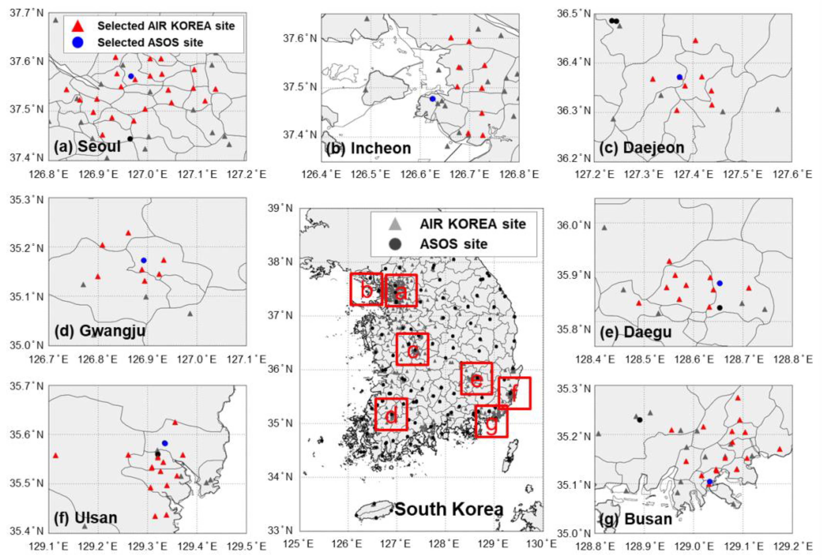
2.1. Dataset

We constructed 3.1-year big data for model development (May 2017 to December 2019) and prediction (November 2016 to April 2017). In this study, the data produced after 2019 were not included in the construction of the big data because of COVID-19 (coronavirus disease 2019)-induced anomalies in air quality patterns. As input variables, NCEP (National Center for Environmental Prediction) GFS (Global Forecast System) forecast, KMA (Korea Meteorological Administration), ASOS (Automated Surface Observing System) observations, and NIER AIR KOREA observations were obtained from their official websites (https://rda.ucar.edu/datasets/ds084.1/, last accessed: 11 November 2022; https://rda.ucar.edu/datasets/ds084.1/, last accessed: 11 November 2022; https://www.airkorea.or.kr/web/, last accessed: 11 November 2022). In order to represent the pressure pattern over East Asia, the latitudinal and longitudinal boundaries of GFS were set from 20° N to 52° N and 96° E to 144° E. The forecast product of GFS has a resolution of 0.25° × 0.25°, respectively (i.e., the dimension of the GFS forecast was 128 × 192). Since the time interval of the GFS forecast is three hours, we performed linear interpolation to estimate the hourly forecast dataset.
Figure 1 presents locational information of ASOS and AIR KOREA ground monitoring stations, which consist of 103 and 494 monitoring sites throughout South Korea, respectively. ASOS network provides hourly observed meteorological variables, and the AIR KOREA network provides hourly concentrations of air pollutants (refer to Table 2). Among the monitoring sites, the urban observation sites located in seven major cities (with a population of more than one million) in South Korea were selected for daily PM2.5 predictions (refer to Figure 1a–g). For the prediction of citywide PM2.5, the observations of the selected sites located in each city were averaged. Table 2 is the detailed information on input variables.
Similar to this study, several previous studies have proposed the use of the integration of input features of both observation-based meteorological and air quality information for more accurate DNN-based PM2.5 predictions [13,29]. The selected input variables are closely related to the concentrations of PM2.5. For example, wind speed and amount of precipitation can directly represent the intensity of atmospheric turbulent dispersions and wet scavenging processes, and the concentrations of primary pollutants such as CO and SO2 can denote the degree of domestic anthropogenic emissions. In addition, combining input features allows DNN-based models to consider more diverse atmospheric environmental properties. Among the meteorological variables, wind speed, wind direction, pressure, and geopotential height can represent the possibility of long-range transport of air pollutants. Moreover, by co-considering meteorological and air quality variables such as O3, NO2, temperature, and relative humidity, the intensity of atmospheric oxidation processes can be reflected in the DNN-based prediction.
The input variables were normalized before feeding into the CNN+LSTM hybrid model to prevent overestimating the effect of the variables with large-scale values.
x n o r m a l ,   i = x i x m i n , i x m a x , i x m i n , i
here x n o r m a l ,   i is the normalized value of variable i; x i is the value of variable i; x m a x , i and x m i n , i are maximum and minimum values of variable i, respectively. The previous day’s observations and the next day’s geopotential height forecasts were normalized and merged with the next day’s PM2.5-observations.

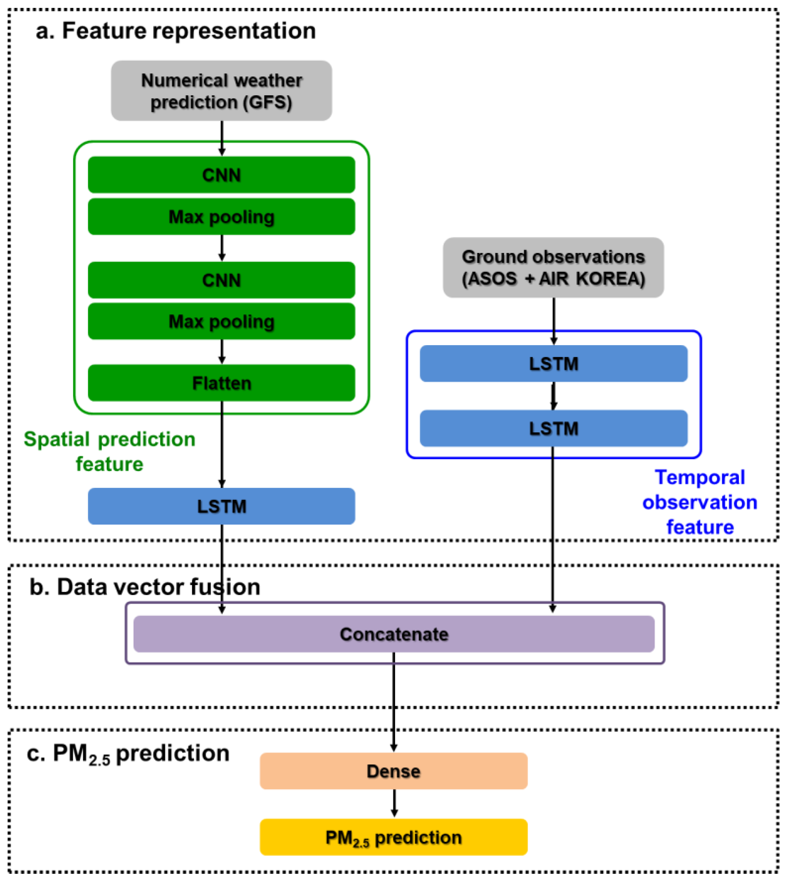
2.2. Model Construction

The procedure of the CNN+LSTM-based daily PM2.5 prediction is summarized in Figure 2. The proposed model consists of three parts: i) feature representation, ii) data vector fusion, and iii) PM2.5 prediction. As shown in the figure, we extracted the spatial feature of the GFS forecast and temporal features of ground observations in the feature representation step. In order to represent the spatial latent features, two CNN layers were embedded. Comprehensive sensitivity tests have been made to determine the number and structure of deep hidden layers. For example, CNN-based autoencoders have been constructed en masse. We elected the type of CNN layers and their structural hyperparameters (the size and number of convolutional filters) based on the reproduction accuracy of the constructed autoencoders. Based on the result, we decided to embed two three-dimensional CNN (3-D CNN) layers to represent the spatial features. The kernel size of CNN layers was set to 3 × 3 × 3. The number of kernels for the first and second CNN layers were 32 and 24. The input dimension of the first 3-D CNN layer was set to 24 × 128 × 192 × 1 for daily PM2.5 prediction. We embedded two 3-D max pooling layers for downscaling the vector matrices extracted from the CNN layers. The pooling size was set to 2 × 2 × 2.
Latent features extracted through convolutional operations were subjected to the next flatten and LSTM layers for data fusion with temporal features. We injected observation-based input features (i.e., ASOS and AIR KOREA observations) into two LSTM-based hidden layers to extract the characteristic of temporal input features. The input dimension of the first LSTM layer was 24 × 14. Additionally, we determined the number of hidden nodes of the entire LSTM layers through sensitive tests. The number of the LSTM hidden nodes was 512. In the second step, the vectors of temporal and spatial latent information extracted through the first step were fused as they passed the concatenate layer. Since the number of LSTM hidden nodes was set to 512, the concatenate layer generates 1024 output vectors. The concatenate layer was connected to the final dense layer. This dense layer identifies the relationship between the outputs of concatenate layer and the true values (observed PM2.5). Table 3 shows the summary of detailed configuration information of the CNN+LSTM hybrid model.
To identify this complicated and non-linear relationship, we need to utilize an activation function for the final dense layer. There are several functions for the activation of DNNs. Among them, rectified linear unit (ReLU) is the most versatile because of its low computation cost [30]. As the output of ReLU ranges from 0 to ∞, its derivative is 0 or 1. Therefore, this function is free from the gradient vanishing and exploding during the back propagations. However, when the hidden node outputs a negative value, the gradient of ReLU is zero, and thus the learnable parameters (weights and biases) associated with the node cannot be adjusted or updated during the model training. In addition, if a huge number of hidden nodes output negative values, training loss can no longer be reduced (i.e., dying ReLU). To prevent the said problem, we used the leaky rectified linear unit (Leaky-ReLU) as the activation function [31]. The Leaky-ReLU expressed by
f ( x ) = { α x                   w h e n   x < 0 x                       w h e n   x 0  
as shown in the equation, the derivative of Leaky-ReLU is α or 1. In this study, we set the value of α as 0.3.

2.3. CNN+LSTM Optimization

Model optimization is a process of finding the optimal combination of weight and bias matrices (learnable parameters). As mentioned previously, the structural hyperparameters of the CNN+LSTM model were determined from the massive amounts of sensitivity tests. There are two main components in DNN optimization: (i) cost function and (ii) optimizer. Their respective roles are to evaluate the accuracy of the updated learnable parameters and to discover efficient and/or stable reduction paths for the cost (or loss). Several cost functions have been utilized in the optimization of DNNs. For better predictive performance, it is very important to select an appropriate objective function corresponding to the purpose of the DNN model. Since the proposed hybrid model was the regression model, the mean squared error (MSE) was utilized as a cost function in this study. The MSE expressed as
J M S E ( θ ) = 1 N i = 1 N ( y i h θ ( x i ) ) 2  
here y i is the true value for i th training; x i is input for i th training; h θ ( x i ) is the predicted value by the given model θ . In this study, adaptive moment estimation (ADAM) was used as an optimizer [32]. The ADAM is an extended stochastic gradient descent algorithm. This algorithm determines the individual adaptive learning rates for different learnable parameters by computing the first and second moments of their gradients.
To train the CNN+LSTM hybrid model, the 2.7-year data (May 2017 to December 2019) were used, as mentioned previously. We divided this dataset into two groups with ratios of 80% for model training and 20% for validation. To confirm the suitability of model optimization, the variations of MSE for model training and validation were monitored during the model training. In the early stage of model optimization, the MSEs of the training and validation decrease together by updating weights and biases. Because training data are only considered in the adjustment of weight and bias matrices, the training cost continuously decreases with the iterative update of learnable parameters. However, the validation MSE decreases until the specific update, and then it stagnates or starts to increase. The optimization of DNNs is to update the learnable parameters until this stagnant or inflection point [33]. If the DNN is properly optimized, the validation MSE at this point should be slightly higher than the training MSE. When the validation MSE is much higher than the training MSE, this represents that the learnable parameters are overturned (i.e., overfitting). On the contrary, if the training cost is bigger than the validation cost, it is called underfitting. From the perspective of improving the predictive performance and generalization of DNNs, it is crucial to minimize the possibility of overfitting and underfitting. To achieve this goal, iterative model training was performed, and then the models with the smallest gap between the training and validation cost were selected for daily PM2.5 prediction. In addition, we also compared the training and validation MSEs and root mean squared errors (RMSEs) to re-evaluate the suitability of model training. The results of this evaluation are summarized in Table 4. Based on this, we confirmed that the CNN+LSTM model was suitably trained.

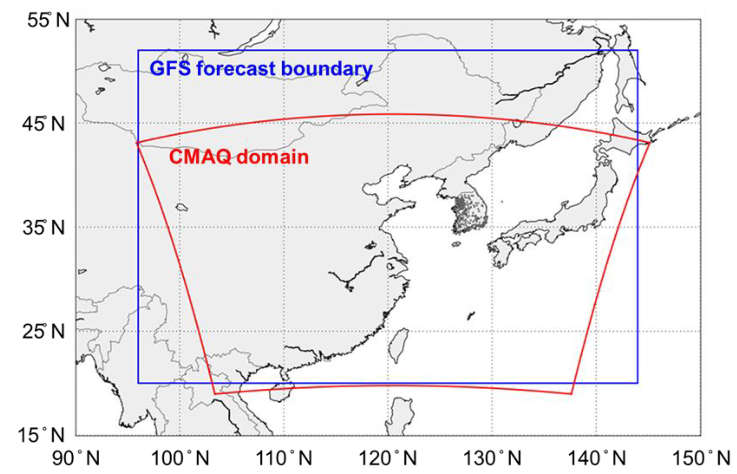
2.4. 3-D CTM-Based PM2.5 Prediction

We made the comparison between the CNN+LSTM-based PM2.5 prediction and the CTM-predicted PM2.5 to evaluate the predictive performance of the CNN+LSTM hybrid neural network model. In this study, we utilized the community multiscale air quality (CMAQ) model v5.2.1 for the 3-D CTM prediction. The meteorological fields for CMAQ prediction were estimated from weather research and forecasting (WRF) v3.8.1 model simulation. Figure 3 presents the boundary of the CMAQ prediction. As shown in the figure, the CMAQ boundary covers northeast Asia. The horizontal resolution of the CMAQ simulation was set to 15 × 15 km2. The KORUS v5.0 emission inventory was used for anthropogenic emissions [34]. The biogenic emissions were acquired from the MEGAN (Model of Emissions of Gases and Aerosols from Nature) v2.1 simulation [35]. The emissions for biomass burning were acquired from FINN (Fire Inventory from National Center for Atmospheric Research, https://www.acom.ucar.edu/Data/fire/, last accesses: 11 November 2022) v1.5 [36]. The lateral boundary conditions were obtained from the official data archive of MOZART-4 (Model for Ozone and Related Chemical Tracers version 4, https://www2.acom.ucar.edu/gcm/mozart-4, last accessed: 11 November 2022), respectively [37].

2.5. Evaluation Metric

In this study, to evaluate the prediction performance of the CNN+LSTM and 3-D CTM, we introduced the following six scientific performance metrics, such as IOA (Index or Agreement), R (Pearson correlation coefficient), RMSE, MB (Mean Bias), MNGE (Mean Normalized Gross Error), and MNB (Mean Normalized Bias). These evaluation metrics were estimated as below:
IOA = 1 i = 1 N ( C M o d e l C O b s ) 2 i = 1 N ( | C M o d e l C O b s ¯ | + | C O b s C O b s ¯ | ) 2
R = i = 1 N ( C M o d e l C M o d e l ¯ ) ( C O b s C O b s ¯ ) i = 1 N ( C M o d e l C M o d e l ¯ ) 2 i = 1 N ( C i , O b s C O b s ¯ ) 2
RMSE = 1 N i = 1 N ( C M o d e l C O b s ) 2  
MB = 1 N   i = 1 N ( C M o d e l C O b s )
MNGE = 1 N   i = 1 N ( | C M o d e l C O b s | C O b s ) × 100
MNB = 1 N   i = 1 N ( C M o d e l C O b s C O b s ) × 100
here C M o d e l and C O b s represent the modeled and observed PM2.5, C M o d e l ¯ and C O b s ¯ are the averaged C M o d e l and C O b s .

3. Results

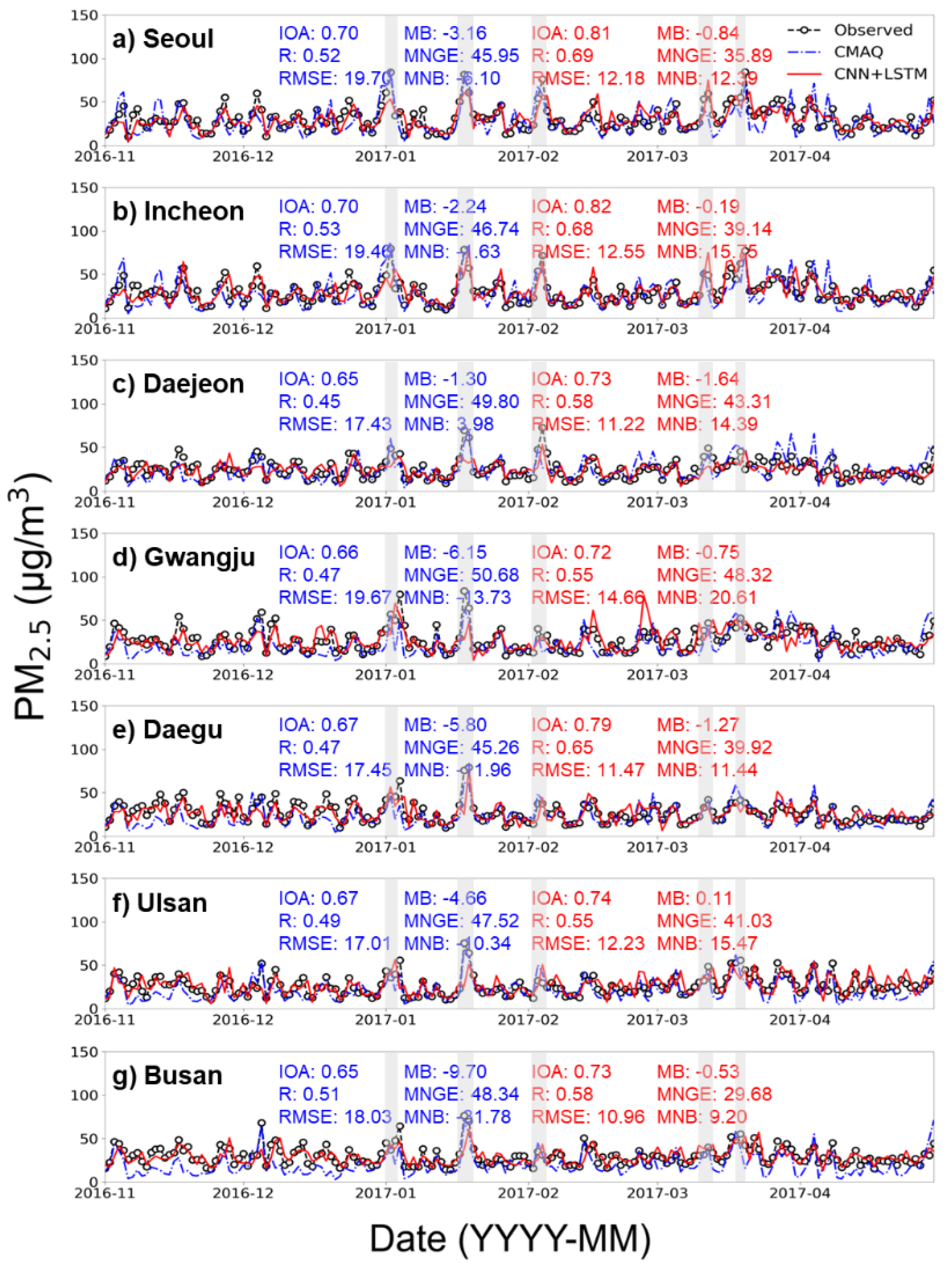
3.1. Model Evaluation

We performed the daily PM2.5 prediction from November 2016 to April 2017. In order to evaluate the accuracy of the newly developed hybrid model, the CNN+LSTM-based PM2.5 was compared to the observed PM2.5. The CNN+LSTM-predicted PM2.5 was also compared with that by CMAQ prediction. The results of this comparison are summarized in Table 5 and also shown in Figure 4. In the figure, the black-dashed line with an open circle represents the observed daily PM2.5; blue-dashed and red lines represent the CMAQ- and CNN+LSTM-predicted daily PM2.5; the grey shade represents the period with relatively high concentration among nationwide high PM2.5 episodes, respectively. As shown in the figure, the CNN+LSTM predictions showed better agreements with the observations compared to the CMAQ-based predictions.
As shown in Figure 4 and Table 5, the CNN+LSTM predicted PM2.5 more accurately than the CMAQ. The IOA for the CNN+LSTM-based PM2.5 prediction ranged from 0.72 to 0.82. On the other hand, the CMAQ-based IOA ranged from 0.65 to 0.70. These differences in IOA demonstrate that the CNN+LSTM can produce 1.10–1.18 times better air quality information than the CMAQ. Based on the statistic metric, among seven cities, the CNN+LSTM predictions (0.81 ≤ IOA ≤ 0.82) at Seoul and Incheon showed the best agreements with the observations. The CMAQ-based predictions in these cities also showed better correlations with the observed PM2.5 (IOA = 0.70). However, the accuracies of the CNN+LSTM at Daejeon, Gwangju, and Busan (0.72 ≤ IOA ≤ 0.73) were relatively low. The CMAQ predictions showed similar trends to the CNN+LSTM-based predictions (0.65 ≤ IOA ≤ 0.66).
In addition, the CNN+LSTM-based predictions showed fewer errors and lower biases. The RMSE for CNN+LSTM predictions ranged from 10.96 μg/m3 to 14.66 μg/m3, and those by CMAQ ranged from 17.01 μg/m3 to 19.70 μg/m3. The CNN+LSTM generated 1.51 times smaller deviation compared to the CMAQ. The prediction errors made by the CNN+LSTM showed significant improvement in Seoul and Busan; the improved rates in these cities were 38.17% and 39.21%. The CNN+LSTM-based predictions also showed lower biases than the CMAQ-based estimations. The MBs for the CMAQ predictions ranged from −9.70 μg/m3 to −1.30 μg/m3. These negative MBs indicate that the CMAQ model significantly underestimates ambient levels of PM2.5. Although the CNN+LSTM-based predictions also showed negative biases (−1.64 μg/m3 ≤ MB ≤ 0.11 μg/m3), their values were 6.46 times smaller than those predicted by CMAQ.
As mentioned above, the PM2.5 prediction was conducted from November 2016 to April 2017. During this cold season, high PM2.5 events (PM2.5 ≥ 40 μg/m3) occur frequently in South Korea. There were seventeen nationwide high PM2.5 episodes. These high episodes are mainly attributable to the long-range transport of air pollutants by highly enhanced westerly wind and increased consumption of fossil fuels for domestic heating [22]. In particular, the daily PM2.5 in Seoul increased up to 85 μg/m3 on January 1 and March 20, respectively. As shown in Figure 4, the CNN+LSTM model generated relatively high errors and biases during the nationwide high-PM events. Since DNNs optimize their weight and bias matrices in a data-driven manner, the corresponding errors and biases arise from the quality of the optimization dataset. Because DNNs are black box models, accurate investigation of data quality is practically impossible.
In this study, to indirectly present the data quality, we evaluated the data imbalance. The datasets used for the optimization of the CNN+LSTM model were highly imbalanced (i.e., the majority class of the training data consisted of the data samples with a relatively low concentration of PM2.5). Since DNNs make predictions based on statistically generalized non-linear relationships between input features, it is difficult for the influence of minority-class data samples to be reflected in their estimations. The data samples with high PM2.5 contributed just 11.30% on average. Among the seven training datasets, the training data for Seoul and Gwangju included the highest number of high-PM2.5 incident samples; their contribution was 12.32% and 12.10%, respectively. In addition, Daejeon showed the lowest frequency of high-PM2.5 incident samples (9.14%). However, as mentioned above, data imbalance is only an indirect indicator of data quality. Therefore, it is logically flawed to conclude that the cause of the performance degradation of the CNN+LSTM is entirely due to the said indicator.

3.2. Importance of Input Features

It is impossible to directly comprehend the relationship between input features and predictions of the DNNs due to the complex non-linearity between the outputs of the deeply structured hidden layers. In this study, we indirectly evaluated the influence of the input variables by sequential perturbing each feature. The main idea of this method is that: if the perturbed feature is “important” (i.e., an input feature has a larger influence on performance), the accuracy of the model predictions will be greatly reduced by the perturbation. In contrast, if the perturbed input feature is unnecessary, the predictive performance of the model will be rather improved. In this estimation, IOA was used as a basis for feature importance investigation because it can represent the overall accuracy of model prediction, as the statistical metric includes an error, bias, and correlation. The feature importance was estimated as below:
F I i = ( IOA w / o     p u r t b IOA i ,     p u r t b ) IOA w / o     p u r t b × 100
here F I i is the importance of feature i ; IOA i ,   p u r t b and IOA w / o   p u r t b are accuracies of the CNN+LSTM model with and without perturbation of feature i , respectively. The results of this estimation are summarized in Table 6.
As shown in Table 6, the importance of all input variables was positive. These positive values indicate that all input variables are necessary for daily PM2.5 prediction (i.e., the appropriateness of variable selection). Among the atmospheric environmental variables, the previous day’s PM2.5 and O3 showed a great influence on the next day’s PM2.5. Their importance ranged from 31.67% to 41.82% and from 3.33% to 15.73%, respectively. In particular, the previous-day-PM2.5 was the most important input variable. Among the meteorological variables, PM2.5 prediction was greatly influenced by geopotential height (from 7.92% to 25.29%) and temperature (from 3.10% to 12.87%). In particular, the importance of atmospheric pressure-related features was relatively higher compared to other meteorological variables. This result represents the importance of pressure patterns over East Asia and inside cities in the daily PM2.5 prediction in South Korea. Therefore, the spatial and temporal pressure features should be included as the input variables in the construction of the DNN-based PM2.5 model, and it is essential to embed CNN and LSTM together to extract their inherent information.

4. Conclusions

In this study, we developed a new CNN+LSTM hybrid neural network for daily PM2.5 prediction. The performance of the CNN+LSTM model was precisely evaluated by comparing the CNN+LSTM-based PM2.5 with the ground observations. In addition, the accuracy of the CNN+LSTM was compared with that of CMAQ to prove its usefulness as an air quality prediction tool. The CNN+LSTM hybrid model generated 1.51 and 6.46 times less error and lower bias on average than the CMAQ. In particular, based on IOA, the CNN+LSTM predictions were 1.10–1.18 times more accurate than the CMAQ estimations. This promising result clearly demonstrates that the DNN-based prediction model can be utilized as an effective tool for air quality prediction. In addition, a similar CNN+LSTM model can also be used in the prediction of other harmful air pollutants (e.g., NO2, SO2, and O3).
In particular, the newly developed CNN+LSTM model is more cost-effective than the 3-D CTMs. Several pre-processing steps are required to generate a 3-D CTM-based air quality forecast: simulation of the numerical weather prediction model, preparation of biogenic and anthropogenic emission inventories, acquisition of initial and boundary conditions, and chemical speciation of air pollutants. Despite the efforts of these sophisticated pre-processings, the current 3-D CTM showed lower predictive power than the CNN+LSTM (refer to Section 3.1). On the other hand, the pre-processing of the CNN+LSTM-based prediction is very simple. For PM2.5 predictions, it is only necessary to acquire the observational and forecast-based datasets from their official archives and configure input features. Nevertheless, the current CNN+LSTM model is superior to the 3-D CTM. Because of these advantages, for developing countries where it is impossible to establish and operate their own 3-D CTM-based forecast system due to financial limitations, the CNN+LSTM model developed through this study can be used as a more economical and efficient air quality forecast tool.
Although the current hybrid model can accurately predict PM2.5, its performance can be deteriorated by two obstacles: i) the amount of available data and ii) an imbalance in training data. As shown in Section 3.1, the prediction accuracy of the CNN+LSTM model was very high for medium and relatively low concentrations (PM2.5 < 40 μg/m3). In contrast, the CNN+LSTM tends to generate relatively high errors and biases for high PM2.5 episodes. This inaccuracy originates from the amount and quality of the training data. The NIER of South Korea has officially conducted ground-based PM2.5 monitoring since 2016. Although the PM2.5 observations have been accumulated for seven years up to date, the amount of useful data for the CNN+LSTM development is less than four years, excluding the COVID-19 period. In addition, the data samples with high PM2.5 only contributed 11.30% of the total available observations. Since DNNs statistically determine their predictions, it is very difficult to reflect the influence of these minority classes in the model estimation. In other words, from the perspective of the DNN generalization, the high PM2.5 samples are likely to be recognized as noise signals during the model training. We believe that the current CNN+LSTM hybrid model can be more accurate by acquiring more data samples of minority classes through more observations.

Author Contributions

Conceptualization, H.S.K.; methodology, H.S.K., K.M.H. and J.Y.; software, H.S.K. and J.K.; validation, K.K. and H.K.; writing—original draft preparation, H.S.K. All authors have read and agreed to the published version of the manuscript.

Funding

This research was supported by Basic Science Research Program through the National Research Foundation of Korea (NRF) funded by the Ministry of Education (2022R1I1A1A01066083).

Institutional Review Board Statement

Not applicable.

Informed Consent Statement

Not applicable.

Data Availability Statement

Not applicable.

Acknowledgments

We obtained KMA ASOS, NIER AIR KOREA, and NCEP GFS datasets from respective official data archives. This work appreciates the said institutions for the provision of useful data.

Conflicts of Interest

The authors declare no conflict of interest.

References

  1. Dorkery, D.W.; Schwartz, J.; Spengler, J.D. Air pollution and daily mortality: Associations with particles and acid aerosols. Environ. Res. 1992, 59, 362–373. [Google Scholar] [CrossRef] [PubMed]
  2. Pope III, C.A.; Dorkey, D.W. Health effects of fine particulate air pollution: Lines that connect. J. Air Waste Manag. Assoc. 2006, 56, 709–742. [Google Scholar] [CrossRef] [PubMed]
  3. Berge, E.; Huang, H.-C.; Chang, J.; Liu, T.-H. A study of the importance of initial conditions for photochemical oxidant modeling. J. Geophys. Res.-Atmos. 2001, 106, 1347–1363. [Google Scholar] [CrossRef]
  4. Liu, T.-H.; Jeng, F.-T.; Huang, H.-C.; Berger, E.; Chang, J.S. Influences of initial conditions and boundary conditions on regional and urban scale Eulerian air quality transport model simulations. Chem.-Glob. Change Sci. 2001, 3, 175–183. [Google Scholar] [CrossRef]
  5. Holloway, T.; Spak, S.N.; Barker, D.; Bretl, M.; Moberg, C.; Hayhoe, K.; van Dorn, J.; Wuebbles, D. Change in ozone air pollution over Chicago associated with global climate change. J. Geophys. Res.-Atmos. 2008, 113, D22306. [Google Scholar] [CrossRef] [Green Version]
  6. Han, K.M.; Lee, C.K.; Lee, J.; Kim, J.; Song, C.H. A comparison study between model-predicted and OMI-retrieved tropospheric NO2 columns over the Korean peninsula. Atmos. Environ. 2011, 45, 2962–2971. [Google Scholar] [CrossRef]
  7. Joharestani, Z.M.; Cao, C.; Ni, X.; Bashir, B.; Talebiesfandarani, S. PM2.5 prediction based on random forest, XGBoost, and deep learning using multisource remote sensing data. Atmosphere 2019, 10, 373. [Google Scholar] [CrossRef] [Green Version]
  8. Karimian, H.; Li, Q.; Wu, C.; Qi, Y.; Mo, Y.; Chen, G.; Zhang, X.; Sachdeva, S. Evaluation of different machine learning approaches to forecasting PM2.5 mass concentrations. Aerosol Air Qual. Res. 2019, 19, 1400–1410. [Google Scholar] [CrossRef] [Green Version]
  9. Li, T.; Hua, M.; Wu, X. A hybrid CNN-LSTM model for forecasting particulate matter (PM2.5). IEEE Access 2020, 8, 26933–26940. [Google Scholar] [CrossRef]
  10. Park, U.; Ma, J.; Ryu, U.; Ryom, K.; Juhyok, U.; Park, K.; Park, C. Deep learning-based PM2.5 prediction considering the spatiotemporal correlations: A case study of Beijing, China. Sci. Total Environ. 2020, 699, 133561. [Google Scholar] [CrossRef]
  11. Al-Alawi, S.M.; Abdul-Wahab, S.A.; Bakheit, C.S. Combining principal component regression and artificial neural networks for more accurate predictions of ground-level ozone. Environ. Model. Softw. 2008, 23, 396–403. [Google Scholar] [CrossRef]
  12. Feng, y.; Zhang, W.; Sun, D.; Zhang, L. Ozone concentration forecast method based on genetic algorithm optimized back propagation neural networks and support vector machine data classification. Atmos. Environ. 2011, 45, 1979–1985. [Google Scholar] [CrossRef]
  13. Kim, H.S.; Park, I.; Song, C.H.; Lee, K.; Yun, J.W.; Kim, H.K.; Jeon, M.; Lee, J.; Han, K.M. Development of a daily PM10 and PM2.5 prediction system using a deep long short-term memory neural network model. Atmos. Chem. Phys. 2019, 19, 12935–12951. [Google Scholar] [CrossRef] [Green Version]
  14. Zhao, j.; Deng, F.; Cai, Y.; Chen, J. Long short-term memory—Fully connected (LSTM-FC) neural network for PM2.5 concentration prediction. Chemosphere 2019, 220, 486–492. [Google Scholar] [CrossRef] [PubMed]
  15. Chang-Hoi, H.; Park, I.; Oh, H.-R.; Gim, H.J.; Hur, S.K.; Kim, J.; Choi, D.-R. Development of a PM2.5 prediction model using a recurrent neural network algorithm for the Seoul metropolitan area, Republic of Korea. Atmos. Environ. 2021, 245, 118021. [Google Scholar] [CrossRef]
  16. Muruganandam, N.S.; Arumugam, U. Seminal stacked long short-term memory (SS-LSTM) model for forecasting particulate matter (PM2.5 and PM10). Atmosphere 2022, 13, 1726. [Google Scholar] [CrossRef]
  17. Eslami, E.; Choi, Y.; Lops, Y.; Sayeed, A. A real-time hourly ozone prediction system using deep convolutional neural network. Neural Comput. Appl. 2020, 32, 8783–8797. [Google Scholar] [CrossRef] [Green Version]
  18. Park, Y.; Kwon, B.; Heo, J.; Hu, X.; Liu, Y.; Moon, T. Estimating PM2.5 concentration of the conterminous United States via interpretable convolutional neural networks. Environ. Pollut. 2020, 256, 113395. [Google Scholar] [CrossRef]
  19. Dai, H.; Huang, G.; Wang, J.; Zeng, H.; Zhou, F. Prediction of air pollutant concentration based on one-dimensional multi-scale CNN-LSTM considering spatial-temporal characteristics: A case study of Xi’an, China. Atmosphere 2021, 12, 1626. [Google Scholar] [CrossRef]
  20. Connor, J.T.; Martin, R.D.; Atlas, L.E. Recurrent neural networks and robust time series prediction. IEEE Trans. Neural Netw. 1994, 5, 240–254. [Google Scholar] [CrossRef]
  21. Sezer, O.B.; Gudelek, M.U.; Ozbayoglu, A.M. Financial time series forecasting with deep learning: A systematic literature review: 2005–2019. Appl. Soft. Comput. 2020, 90, 106181. [Google Scholar] [CrossRef] [Green Version]
  22. Hochreiter, S.; Schmidhuber, J. Long short-term memory. Neural Comput. 1977, 9, 1735–1780. [Google Scholar] [CrossRef] [PubMed]
  23. Graves, A. Long short-term memory. In Supervised Sequence Labelling with Recurrent Neural Networks; Springer: Berlin, Germany, 2012; Volume 385, pp. 37–45. [Google Scholar]
  24. Sak, H.; Senior, A.; Beaufays, F. Long short-term memory based recurrent neural network architectures for large vocabulary speech recognition. arXiv 2014, arXiv:1402.1128. [Google Scholar]
  25. Albawi, S.; Mohammed, T.A.; Al-Zawi, S. Understanding of a convolutional neural network. In Proceedings of the 2017 International Conference on Engineering and Technology (ICET), Antalya, Turkey, 21–23 August 2017. [Google Scholar]
  26. Gu, J.; Wang, Z.; Kuen, J.; Ma, L.; Shahroudy, A.; Shuai, B.; Liu, T.; Wang, X.; Wang, G.; Cai, J.; et al. Recent advances in convolutional neural networks. Pattern Recognit. 2018, 77, 354–377. [Google Scholar] [CrossRef] [Green Version]
  27. Rawat, W.; Wang, Z. Deep convolutional neural networks for image classification: A comprehensive review. Neural Comput. 2017, 29, 2352–2449. [Google Scholar] [CrossRef]
  28. Kim, H.C.; Kim, E.; Bae, C.; Cho, J.H.; Kim, B.-U.; Kim, S. Regional contributions to particulate matter concentration in the Seoul metropolitan area, South Korea: Seasonal variation and sensitivity to meteorology and emissions inventory. Atmos. Chem. Phys. 2017, 17, 10315–10332. [Google Scholar] [CrossRef] [Green Version]
  29. Sayeed, A.; Lops, Y.; Choi, Y.; Jung, J.; Salman, A.K. Bias correcting and extending the PM forecast by CMAQ up to 7 days using deep convolutional neural networks. Atmos. Environ. 2021, 253, 118376. [Google Scholar] [CrossRef]
  30. Nair, V.; Hinton, G.E. Rectified linear units improve restricted Boltzmann machines. In Proceedings of the 27th International Conference on Machine Learning, Haifa, Israel, 21–24 June 2010. [Google Scholar]
  31. Mass, A.L.; Hannun, A.Y.; Ng, A.Y. Rectifier nonlinearities improve neural network acoustic models. In Proceedings of the 30th International Conference on Machine Learning, Atlanta, GA, USA, 16–21 June 2013. [Google Scholar]
  32. Kingma, D.; Ba, J. A method for stochastic optimization. In Proceedings of the 3rd International Conference on Learning Representations, San Diego, CA, USA, 3–8 May 2015. [Google Scholar]
  33. Mahsereci, M.; Ballers, L.; Lassner, C.; Henning, P. Early stopping without a validation set. arXiv 2017, arXiv:1703.09580. [Google Scholar]
  34. Woo, J.-H.; Kim, Y.; Kim, H.-K.; Choi, K.-C.; Eum, J.-H.; Lee, J.-B.; Lim, J.-H.; Kim, J.; Seong, M. Development of the CREATE Inventory in Support of Integrated Climate and Air Quality Modeling for Asia. Sustainability 2020, 12, 7930. [Google Scholar] [CrossRef]
  35. Guenther, A.; Karl, T.; Harley, P.; Wiedinmyer, C.; Palmer, P.I.; Geron, C. Estimates of global terrestrial isoprene emissions using MEGAN (Model of Emissions of Gases and Aerosols from Nature). Atmos. Chem. Phys. 2006, 6, 3181–3210. [Google Scholar] [CrossRef] [Green Version]
  36. Wiedinmyer, C.; Akagi, S.K.; Yokelson, R.J.; Emmons, L.K.; Al-Saadi, J.A.; Orlando, J.J.; Soja, A.J. The Fire INventory from NCAR (FINN): A high resolution global model to estimate the emissions from open burning. Geosci. Model Dev. 2011, 4, 625–641. [Google Scholar] [CrossRef] [Green Version]
  37. Emmons, L.K.; Walters, S.; Hess, P.G.; Lamarque, J.-F.; Pfister, G.G.; Fillmore, D.; Granier, C.; Guenther, A.; Kinnison, D.; Laepple, T.; et al. Description and evaluation of the Model for Ozone and Related chemical Tracers, version 4 (MOZART-4). Geosci. Model Dev. 2010, 3, 43–67. [Google Scholar] [CrossRef]
Figure 1. Locations of KMA ASOS and NIER AIR KOREA observation sites in seven major cities: (a) Seoul, (b) Incheon, (c) Daejeon, (d) Gwangju, (e) Daegu, (f) Ulsan, and (g) Busan. The blue circle represents the ASOS site, and the red triangle represents the AIR KOREA site.
Atmosphere 13 02124 g001
Figure 2. Flowchart of the CNN+LSTM hybrid ANN-based PM2.5 prediction.
Atmosphere 13 02124 g002
Figure 3. Boundary of the CMAQ prediction (red line) and GFS forecast (blue line). The grey triangles and dots represent the locational information of ground monitoring stations in South Korea.
Atmosphere 13 02124 g003
Figure 4. Comparisons between the observed, CMAQ-predicted, and the CNN+LSTM-predicted PM2.5 at seven major cities in South Korea. Black-dashed line with an open circle represents the observed PM2.5. A blue-dashed line represents the CMAQ-predicted PM2.5. A red line represents the CNN+LSTM-predicted PM2.5. Grey shade represents the period with relatively high concentration among nationwide high PM2.5 episodes.
Atmosphere 13 02124 g004
Table 1. Performance comparison between AI-based PM2.5 prediction models *.
ReferencesStudy AreaPeriodAlgorithmRMSE (μg/m3)
Joharestani et al., 2019 [7]Tehran, Iran2015–2018Random forest14.47
XGBoost13.66
MLP15.11
Karimian et al., 2019 [8]Tehran, Iran2013–2016MART13.19
DFFN19.62
LSTM9.42
Li et al., 2020 [9]Beijing, China2010–2014CNN+LSTM17.93
LSTM18.08
Park et al., 2020 [10]Beijing, China2015–2017MLP37.79
LSTM11.34
CNN+LSTM5.357
* XGBoost stands for extreme gradient boosting; MLP stands for multi-layer perceptron; MART stands for multiple additive regression trees; DFFN stands for deep feed forward neural network.
Table 2. Input variables of CNN+LSTM hybrid PM2.5 prediction model.
Data TypeVariableUnitTime ResolutionFeature Type
Observed meteorological variableTemperatureK1 hTemporal feature
Wind speedm/s
Wind direction°
Relative humidity%
Vapor pressurehPa
Dew pointK
PressurehPa
Sea level pressurehPa
Observed atmospheric
environmental variable
SO2ppmv1 hTemporal feature
COppmv
O3ppmv
NO2ppmv
PM10μg/m3
PM2.5μg/m3
Predicted meteorological variableGeopotential height *gpm3 hSpatial feature
* Geopotential height at 850 hpa.
Table 3. Configuration of the CNN+LSTM hybrid neural network model.
Prediction StepStructural
Hyperparameter
Neural Network
1st CNN1st Max Polling2nd CNN2nd Max PollingFlattenLSTM
Feature
representation for spatial
features
Input shape(None, 24, 128, 192, 1)(None, 24, 128, 192, 32)(None, 12, 64, 96, 32)(None, 12, 64, 96, 24)(None, 6, 32, 48, 24)(None, 221184)
CNN kernels or hidden nodes32-24--512
Kernel size(3, 3, 3)-(3, 3, 3)---
ActivationReLU-ReLU--Tanh
Pooling size-(2, 2, 2)-(2, 2, 2)--
Output shape(None, 24, 128, 192, 32)(None, 12, 64, 96, 32)(None, 12, 64, 96, 24)(None, 6, 32, 48, 24)(None, 221184)(None, 512)
Feature
representation for temporal
features
1st LSTM2nd LSTM
Input shape(None, 24, 14)(None, 24, 512)
Hidden nodes512512
ActivationTanhTanh
Output shape (None, 24, 512) (None, 512)
Data vector
fusion
Concatenate layer
Input shape[(None, 512), (None, 512)]
Output shape(None, 1024)
PM2.5 prediction Final dense layer
Input shape(None, 1024)
Hidden nodes24
ActivationLeaky-ReLU
Output shape(None, 24)
Table 4. Evaluation of the suitability of model optimization *.
CityTrainingValidation
MSERMSEMSERMSE
Seoul131.8511.48152.8112.36
Incheon133.2111.54145.9812.08
Daejeon95.049.7598.659.93
Gwangju105.7210.28127.6311.30
Daegu87.579.3696.209.81
Ulsan101.6010.08112.5110.61
Busan124.0911.14140.8411.87
* The units of MSE and RMSE are μg/m3.
Table 5. Scientific evaluations of the CMAQ- and CNN+LSTM-based PM2.5 predictions *.
ModelCityStatistical Parameters
IOARRMSEMBMNGEMNB
CMAQSeoul0.700.5219.70−3.1645.95−6.10
Incheon0.700.5319.46−2.2446.74−1.63
Daejeon0.650.4517.43−1.3049.803.98
Gwangju0.660.4719.67−6.1550.68−13.73
Daegu0.670.4717.45−5.8045.26−11.96
Ulsan0.670.4917.01−4.6647.52−10.34
Busan0.650.5118.03−9.7048.34−31.78
CNN+LSTMSeoul0.810.6912.18−0.8435.8912.39
Incheon0.820.6812.55−0.1939.1415.75
Daejeon0.730.5811.22−1.6443.3114.39
Gwangju0.720.5514.66−0.7548.3220.61
Daegu0.790.6511.47−1.2739.9211.44
Ulsan0.740.5512.230.1141.0315.47
Busan0.730.5810.96−0.5329.689.20
* The unit for RMSE and MB is μg/m3; the unit for MNGE and MNB is %.
Table 6. Importance of the input features in daily PM2.5 prediction *.
TypeInput FeatureFeature Importance
SeoulIncheonDaejeonGwangjuDaeguUlsanBusan
Meteorological variableGeopotential height25.2922.0021.8636.417.9215.0414.32
Temperature12.8712.549.829.714.703.105.95
Wind speed0.160.190.060.130.140.140.06
Wind direction1.863.900.302.222.711.290.48
Relative humidity1.861.847.407.883.657.793.65
Vapor pressure7.687.586.435.526.988.030.04
Dew point2.082.230.472.231.103.602.30
Pressure3.254.994.506.917.051.293.36
Sea level pressure2.602.372.617.267.292.563.00
Atmospheric
environmental variable
SO22.671.871.866.227.932.912.36
CO1.740.920.283.691.381.960.40
O38.063.3310.4415.736.798.873.66
NO22.260.941.713.793.433.840.33
PM100.961.645.080.771.202.364.58
PM2.538.8038.2434.9341.8237.1734.7931.67
* The unit for feature importance is %.
Publisher’s Note: MDPI stays neutral with regard to jurisdictional claims in published maps and institutional affiliations.

