Article

Short-Term Air Pollution Forecasting Using Embeddings in Neural Networks

by
Enislay Ramentol
1,*,
Stefanie Grimm
1,
Moritz Stinzendörfer
1,2 and
Andreas Wagner
1,3
1
Fraunhofer Institute for Industrial Mathematics ITWM, Department for Financial Mathematics, Fraunhofer-Platz 1, 67663 Kaiserslautern, Germany
2
Department of Mathematics, RPTU Kaiserslautern-Landau, Paul-Ehrlich-Str. 14, 67663 Kaiserslautern, Germany
3
Faculty of Management Science and Engineering, Karlsruhe University of Applied Sciences, Moltkestrasse 30, 76133 Karlsruhe, Germany
*
Author to whom correspondence should be addressed.
Atmosphere 2023, 14(2), 298; https://doi.org/10.3390/atmos14020298
Submission received: 10 January 2023 / Revised: 26 January 2023 / Accepted: 29 January 2023 / Published: 2 February 2023
(This article belongs to the Special Issue Machine Learning in Air Pollution)

Abstract

:
Air quality is a highly relevant issue for any developed economy. The high incidence of pollution levels and their impact on human health has attracted the attention of the machine-learning scientific community. We present a study using several machine-learning methods to forecast NO2 concentration using historical pollution data and meteorological variables and apply them to the city of Erfurt, Germany. We propose modelling the time dependency using embedding variables, which enable the model to learn the implicit behaviour of traffic and offers the possibility to elaborate on local events. In addition, the model uses seven meteorological features to forecast the NO2 concentration for the next hours. The forecasting model also uses the seasonality of the pollution levels. Our experimental study shows that promising forecasts can be achieved, especially for holidays and similar occasions which lead to shifts in usual seasonality patterns. While the MAE values of the compared models range from 4.3 to 15, our model achieves values of 4.4 to 7.4 and thus outperforms the others in almost every instance. Those forecasts again can for example be used to regulate sources of pollutants such as, e.g., traffic.

1. Introduction

Air quality forecasting has become a topic of high interest for all societies since it represents a great threat to health and the climate. Air toxicity kills approximately seven million people worldwide each year, as a result of increased mortality from stroke, heart disease, chronic obstructive pulmonary disease, lung cancer, and acute respiratory infections (https://www.who.int/health-topics/air-pollution, accessed on 10 December 2022). Statistics published by the WHO (World Health Organization) show that nine out of ten people breathe air that contains high levels of pollutants, exceeding the limits of the WHO guidelines. According to the WHO, the top six air pollutants include particulate pollution, ground-level ozone, carbon monoxide, sulphur oxides, nitrogen oxides, and lead. Nitrogen dioxide (NO2) is a gaseous atmospheric pollutant that arises mostly as a result of road traffic and other fossil fuel combustion processes. Its presence in the air helps the formation and modification of other air pollutants, such as ozone and particles, as well as acid rain. The negative effects of NO2 on health have been extensively studied [1,2,3], and authors have shown a high correlation between certain diseases and exposure to high concentrations of NO2 [4,5]. In this research, we focused on the short-term forecast of NO2 in the city of Erfurt, Germany. We forecasted the NO2 concentration for the next 24, 72 or 120 h using a deep-learning (DL) approach, which is based on neural networks and embedding layers to encode time variables. Data access was realised using the standardised OGC SensorThings API (http://docs.opengeospatial.org/is/15-078r6/15-078r6.html, accessed on 10 December 2022) (implemented by FROST https://fraunhoferiosb.github.io/FROST-Server/, accessed on 10 December 2022). Since this covers both the historical sensor data as well as the meteorological variables, all input data could be retrieved through a unified interface. Historical NO2 values were imported from the European Environment Agency (https://datacoveeu.github.io/API4INSPIRE/datanests/ad-hoc.html, accessed on 10 December 2022), whereas the meteorological variables were obtained from Meteomatics (https://www.meteomatics.com/de/, accessed on 10 December 2022), a provider of weather data and forecasts. Our findings are embedded in the project Bauhaus.MobilityLab (https://bauhausmobilitylab.de/, accessed on 10 December 2022), which has the goal of making urban living spaces more liveable. The resulting NO2 forecasts were used, e.g., for measures influencing the inhabitants of the living lab. A further application is to adapt public transport rates to the expected NO2 values. In this way, one can counteract peaks in air toxicity which are dangerous to health. The remainder of this paper is organised as follows. In Section 2, we provide an introduction to the air pollution forecasting task and the current state-of-the-art methods. In Section 3, we analyse the seasonality of the data collected by the sensors in the city of Erfurt. We use graphs to show the high seasonality in our data, as well as the difference that exists between the data of different locations. In Section 4, we introduce deep neural networks, as well as the use of embedding layers to encode categorical variables. In Section 5, we explain the setup of the experimental study, including a description of the benchmark algorithms used for comparison and present and discuss the results.

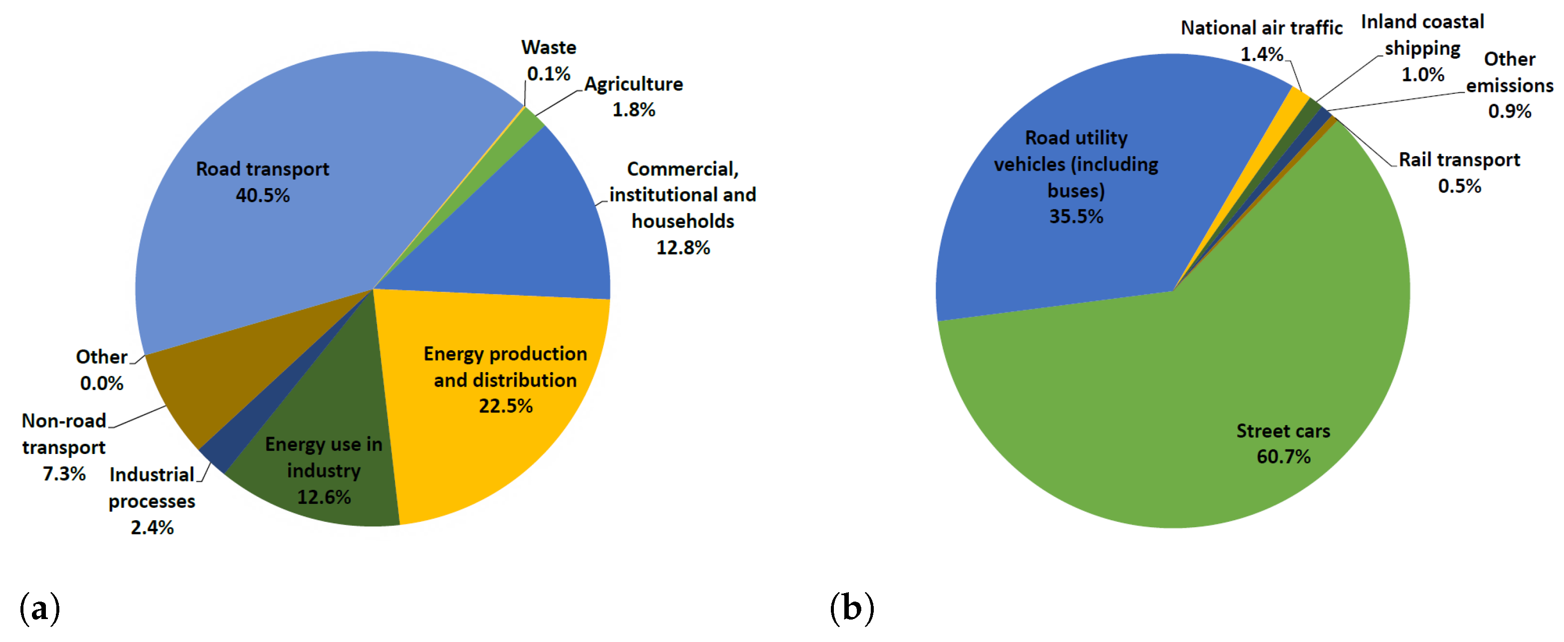
2. NO2 Emissions and Short-Term Forecasting

Our study was focused on NO2, a polluting gas that seriously affects human health. According to international statistics [6], in the year 2019, Germany ranked 22nd in the list of countries that emit the most NO2 per inhabitant, with 13.6 kg per year. Although this number is quite encouraging when compared to the 107.7 kg that each inhabitant of Australia generates, there is still much that can be done to reduce it. Several studies have shown that road traffic has the highest incidence of NO2 emission [7,8,9]. Figure 1a shows the contribution made by different sectors to emissions of nitrogen oxides in 2011. As can be seen, road transport constitutes 41% of total NO2 emissions, being the sector with the most emissions. A study carried out in [10] states that Germany’s climate footprint has improved considerably since the 1990s and that the reasons are mainly the successful reform of the European trade system for emissions, the former low price of gas, the expansion of wind and solar energy and the closure of the first coal-fired power plants. However, the incidence of traffic is still a serious problem, which has been increasing in recent years according to a further study [10].
However, as shown in [10], not all forms of transport pollute to the same level. In Figure 1b, we can see that, at more than 60%, motorised individual transport in the form of cars had the highest incidence of emissions in the transport sector during 2017. In contrast, rail transport contributed only 0.6%. It is important to mention that the fact that the highest incidence is in “street cars” gives us some hope about taking action to reduce emissions. A good example is the city of Stuttgart, Germany. The action plan “Nachhaltig mobil in Stuttgart” (sustainable mobility in Stuttgart) was approved on 18 July 2017, by the Municipal Council. The action plan outlines more than 100 individual measures in nine fields of action including local public transport, individual motorised transport, pedestrian and bicycle traffic, commercial traffic, commuter traffic, city-specific mobility, mobility in the region and public relations work, such as intermodality and networking. The mobility package is complemented by other measures of the “Alliance for Mobility and Clean Air” of the City Council. Optimising traffic flow and changes of the model split have been proven to be the most effective measures with the least negative impact. Our NO2 forecasts were applied to two use cases of the project Bauhaus.MobilityLab which targets an enhanced quality of living in the city of Erfurt. First, to optimise the individual traffic with regards to air quality and second, to change the modal split by giving incentives to people who use public transport when there is bad air quality. For both use cases, good knowledge about the current air quality is required. This also includes a fundamental understanding of the sources and current dispersion of bad air in the city. For example, if we know that tomorrow at 17:00 we will have an excessively high NO2 peak in the inner city, we could try to incorporate this information into route planning algorithms, which then again could prioritise park and ride solutions. These use cases can become blueprints for urban planning in further cities.

Using Machine-Learning to Predict Pollutant Concentrations

The use of machine-learning (ML) has become popular as a powerful tool for accurate forecasts [11,12,13]. In the following, we carry out a review of the most significant methods within the state-of-the-art that make short-term forecasts of pollutants in the air. The short-term forecasting of NO2 concentration has attracted the attention of the scientific community [14,15]. Statistical models have been used widely for prediction tasks. However, recently, ML methods have begun to be used more often [14].
In Table 1, we show some important features about the most representative methods from the state-of-the-art. As can be observed, long short-term memory (LSTM) and light gradient-boosting machine (LGBM) have been widely used in comparative studies. Furthermore, most of the models focus only on predicting NO2 concentrations one hour in advance, which is not functional in our case study. Only four of them, one statistical model and three based on ML, predict 24-h time horizons. Therefore, we used three of those methods in our experimental study. Incorporating other methods might be part of future work.

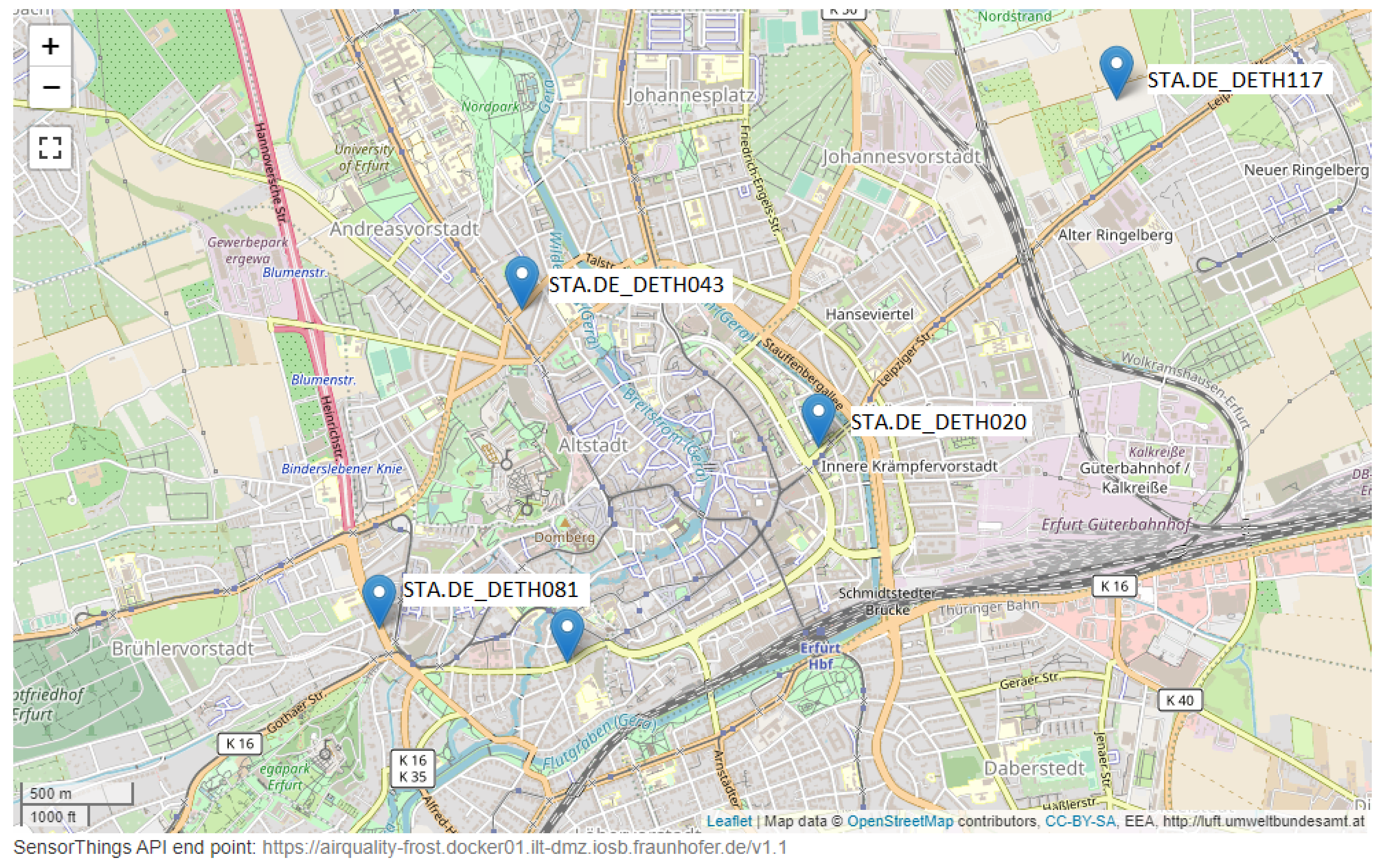
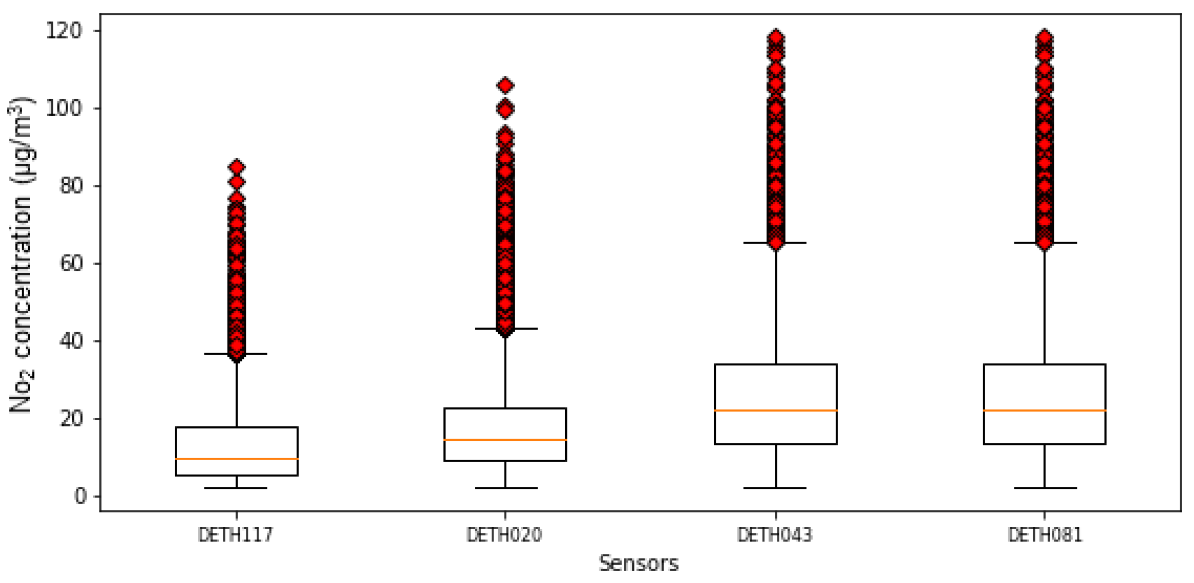
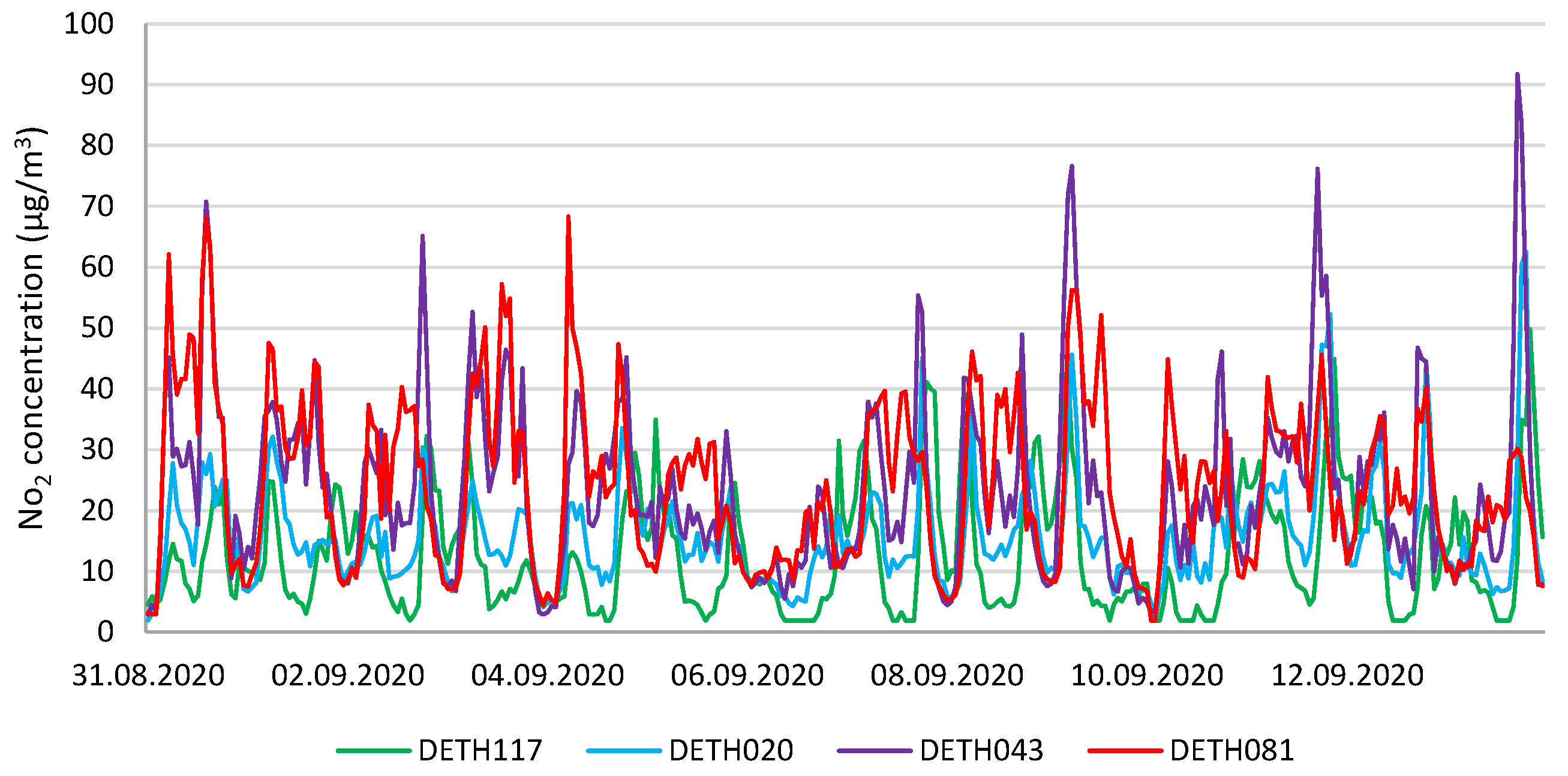
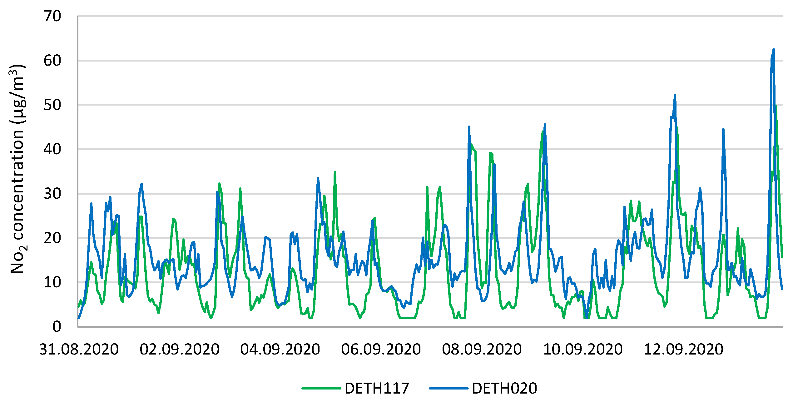
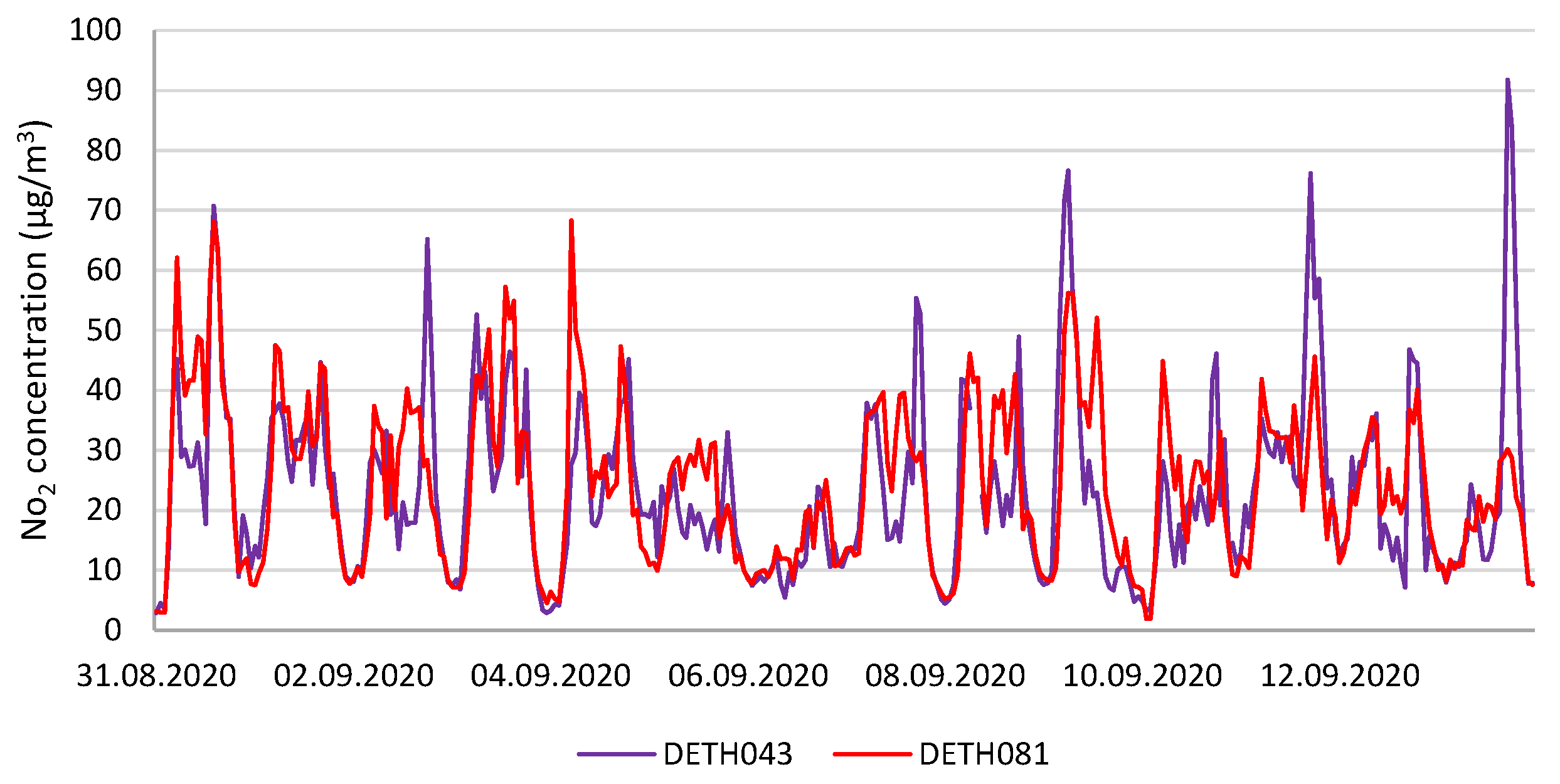
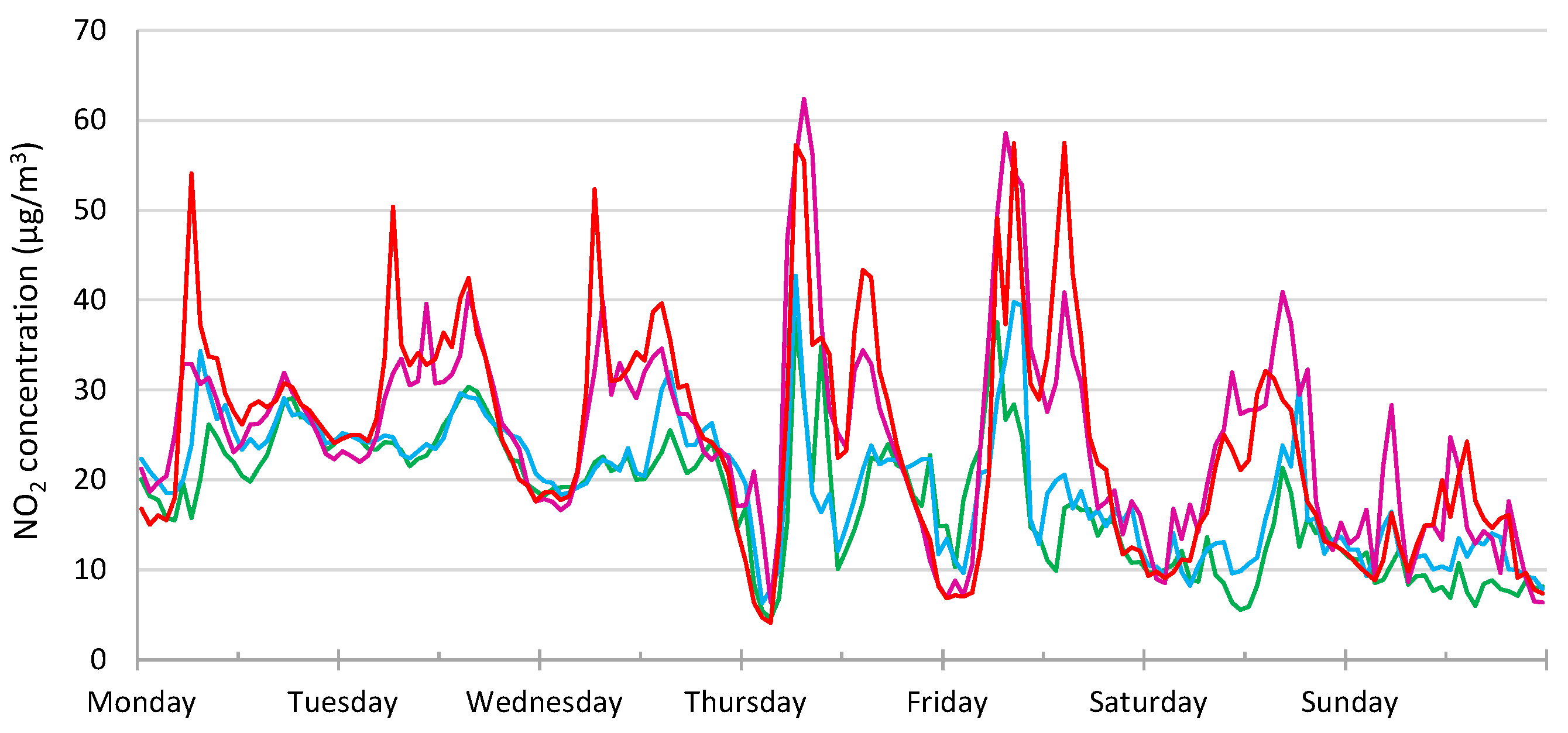
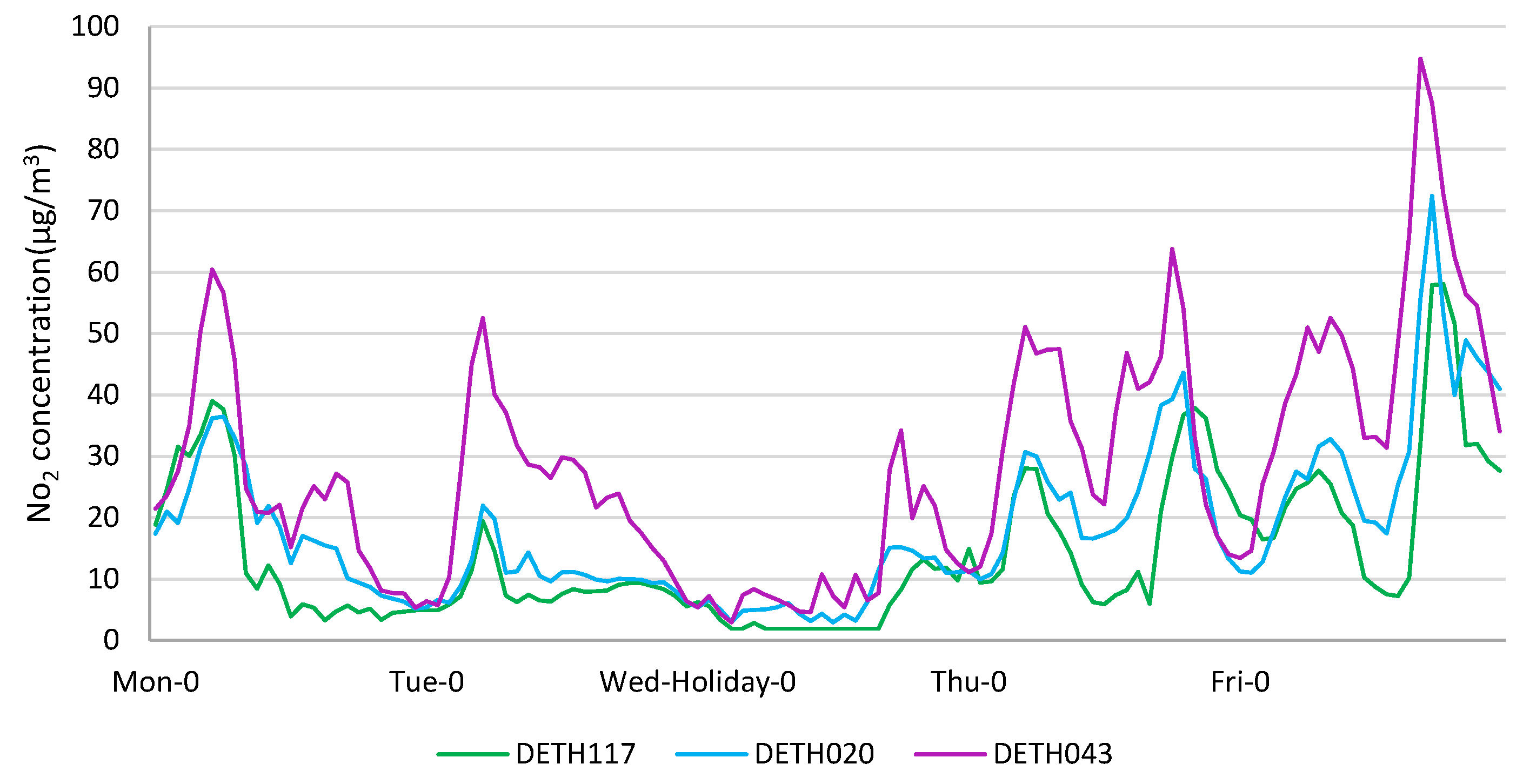
3. NO2 Seasonality Analysis in the City of Erfurt

The analysis of the NO2 concentration was based on four air quality sensors distributed in the city of Erfurt (Figure 2). This data are publicly available from the European Environment Agency (EEA).
In the following we will refer to them by their official names, neglecting the prefix STA.DE:
  • STA.DE_DETH117
  • STA.DE_DETH043
  • STA.DE_DETH020
  • STA.DE_DETH081
Traffic and land use have a high impact on the NO2 concentration [24,25,26]. There are two main factors related to traffic, influencing the NO2 concentration. First, is the location itself. Since most of the NO2 emission is caused by traffic, the distance to main roads and air circulation (dense buildings or rural areas) is a crucial aspect. Second, the air quality is influenced by the amount of traffic. While the location of a sensor is constant, there is a high variation in the traffic over time, due to commuter traffic and working hours or special events.
As can be seen in Figure 2, sensor DETH117 is quite far from the city, so it was expected that it will be the least affected by traffic. Sensor DETH020 is the next farthest from the centre and the busiest highways. On the other hand, sensors DETH081 and DETH043 are located in the city and near important highways. In the case of sensor DETH081, it is located very close to a major highway, the K35 (highlighted in red in Figure 2), so we expected its NO2 concentration measurements to be high. Next, we analysed in detail the data of each sensor, in order to know their characteristics and thus suggest possible ML models that allow accurate forecasts to be made. We analysed the historical NO2 data distribution per sensor in the first step.
The other sensors DETH043 and DETH081 behave in a very similar way, as can be seen in Figure 3. Both have almost the same IQR and average, as well as maximum and minimum values, although the maximum of sensor DETH081 is slightly higher than that of sensor DETH043. These two sensors are the closest to the city (most affected by traffic) and this is evident in the metrics shown by the box plots.
Next, we analysed the relationship between the days of the week and the NO2 level, as well as with holidays. The objective of this analysis was to show the high seasonality of our data and the relationship that exists between the days of the week (including holidays) and the levels of NO2. The study was divided by sensors because each of them is located in a different area and therefore the measurements may be conditioned by different factors.
In Figure 4, we have plotted the NO2 concentrations for the four sensors during the first two weeks of September 2020. For the urban sensors (close to the city) we have used similar colours red and magenta, while for the rural sensors we have used the colours green and blue. As indicated before, the sensors located closer to the urban area show significantly higher concentrations of NO2 than the sensors in rural areas. In Figure 5 and Figure 6, we can observe the differences in details.
The high seasonality of the concentrations of NO2 is a proven fact, as can be seen in Figure 7 and as some authors have previously shown [27]. On weekdays, much higher concentrations are reached than at weekends. Sunday, especially, is a day in which the concentrations of NO2 are very low. We can also observe the existence of two peak times per day, with Thursdays and Fridays being the days when these peaks are highest. Although only one example week is shown in the figure, this pattern is repeated every week of the year, although there are differences between the different seasons of the year. We also observe a difference between the sensors located in urban areas and rural areas. The closer a sensor is located to the city, the higher the NO2 concentration, especially during peak hours.
Another interesting pattern observed in our data is that public holidays have a similar influence as Sundays. The concentration of NO2 is very low compared to the other days of the week. We also observe that those, known as “bridge days”, that is, those days trapped between holidays and weekends, have NO2 concentrations very similar to Saturdays, that is, lower than the other days of the week, but not as low as Sunday. In Figure 8, we have plotted the NO2 concentrations for three of our sensors (Unfortunately for sensor DETH081, it was not possible to retrieve the data for that date) during the week of October 1 to 5, 2018. As seen in Figure 8, despite being Wednesday (a day of very high concentrations), the concentrations are extremely low since October 3rd is a public holiday in Germany (German Unity Day). In Section 6.1, we will address more on this topic.

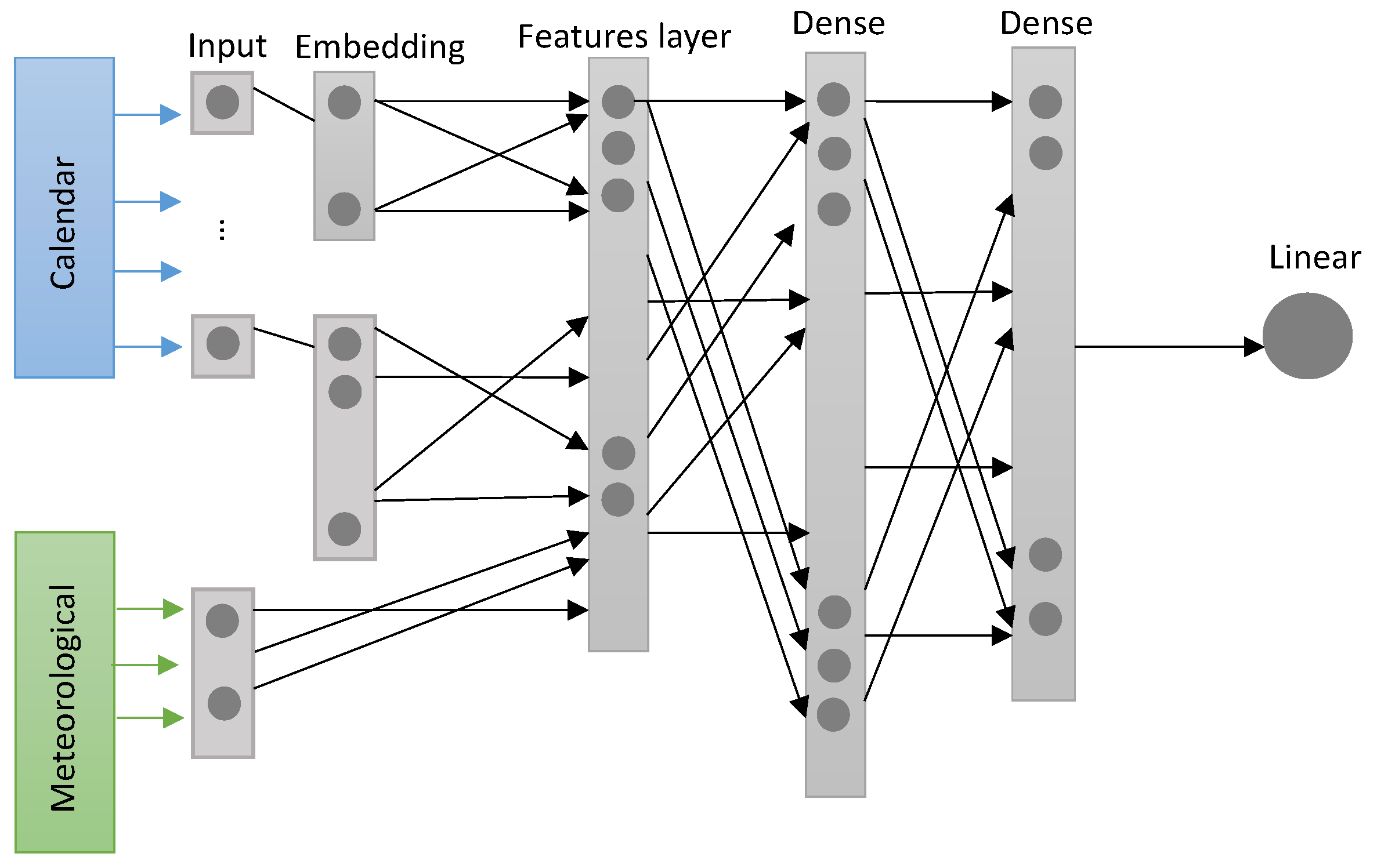
4. On the Use of Embedding Layer in Neural Network: Encoding Traffic

Although neural networks can be considered a fairly old concept in the field of artificial intelligence [28,29], for some years their popularity declined and become practically ignored. However, this began to change in 2006 when Dr. Geoffrey E. Hinton introduced the deep belief networks [30]. It completely revolutionised the area of neural networks, giving rise to deep learning. One of DL’s greatest contributions has been in the area of natural language processing [31], where the introduction of embeddings achieved unprecedented improvement. An embedding is a mapping of a categorical variable to a vector of continuous numbers. In the context of neural networks, embeddings are low-dimensional, learned continuous vector representations of discrete variables [32].

4.1. DNN + Embedding

In this study, we used a dense neuronal network with an embedding layer to encode calendar information. Dense Neuronal Networks (DNN) are fully connected networks. This means each neuron in a layer receives input from all the neurons in the previous layer, as outlined in Figure 9, which shows a representation of our network. Embeddings, as well as meteorological variables, serve as input features (features layer). Finally, we used two hidden layers with Relu-activation (Rectified Linear Unit). The output was one neuron with linear activation.

Embedding Layer for Calendar Features
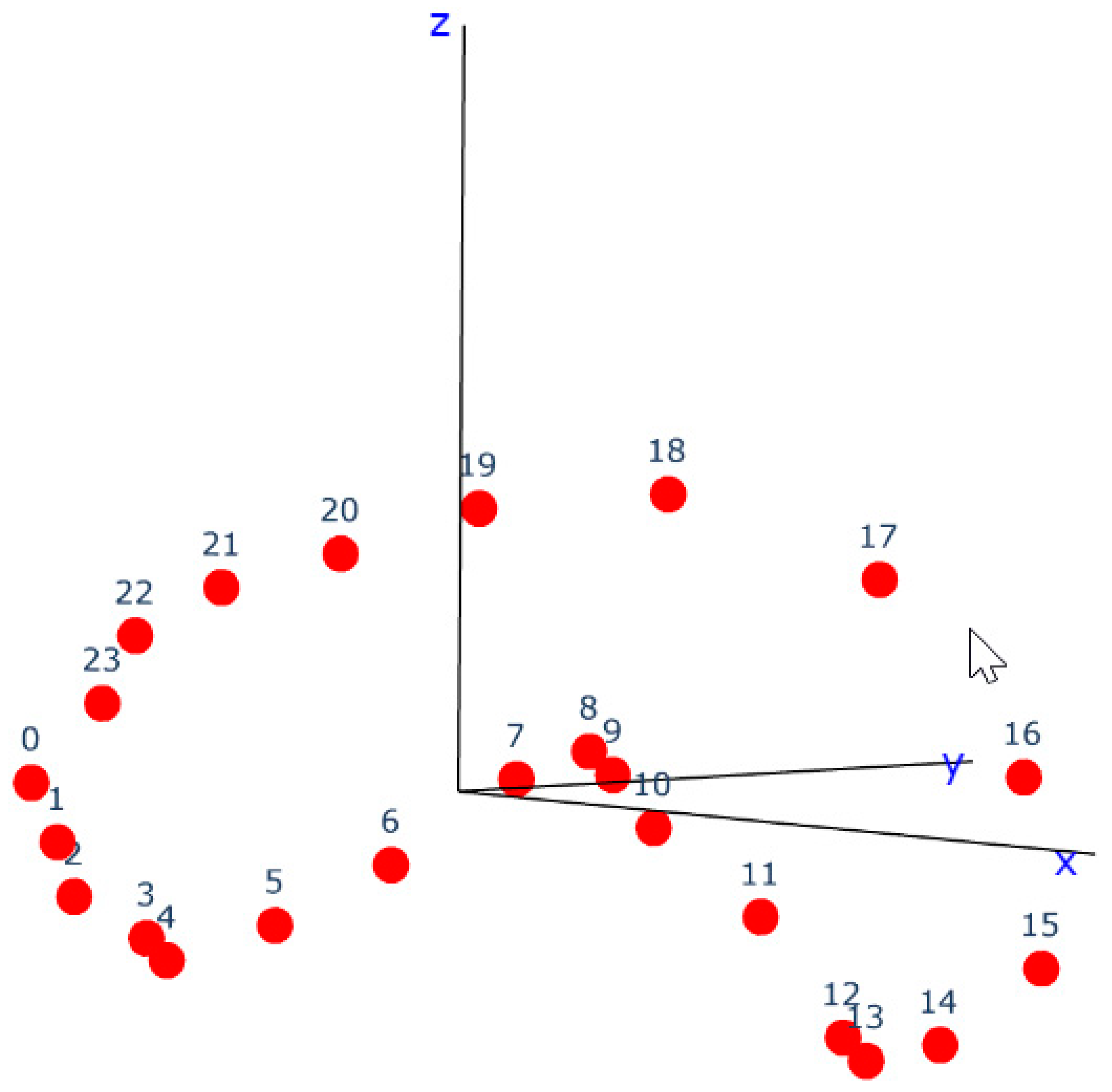
The embedding layer was used to encode calendar information. We considered the following embedding variables:
  • Hour: The categorical variable h o u r takes values in 0 23 , so in a one-hot-encoding it has dimension 24. For its embedding dimension, we chose six, which follows recommendations to use 25 % of the input dimension for the embedding space [33].
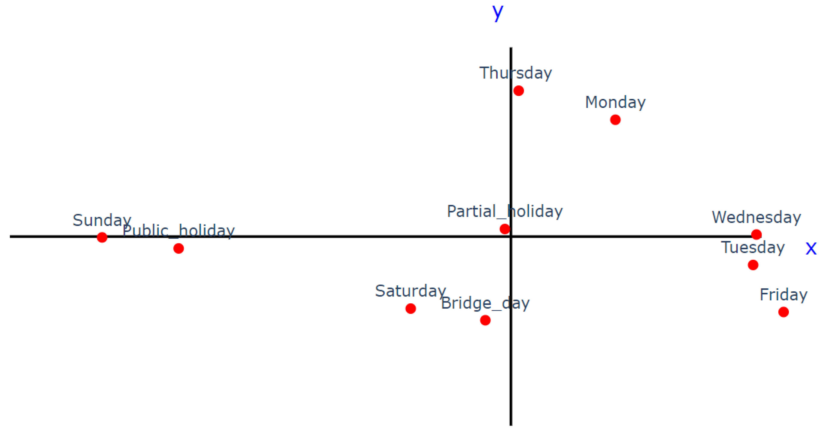
  • Weekday: The categorical variable w e e k d a y takes values in 0 N , where N depends on the representation of holidays outlined below. Its dimension is two. In our study, we defined: weekday as 0 9 , considering seven weekdays and three types of holiday; partial holiday, public holiday and bridge day (bridge, partial, and public holiday describe days with influence through public holidays; public is the actual public holiday, partial is a public holiday in only parts of Germany and bridge describes days between a public holiday and weekends). A list of holidays used in this study can be found in the Appendix A.
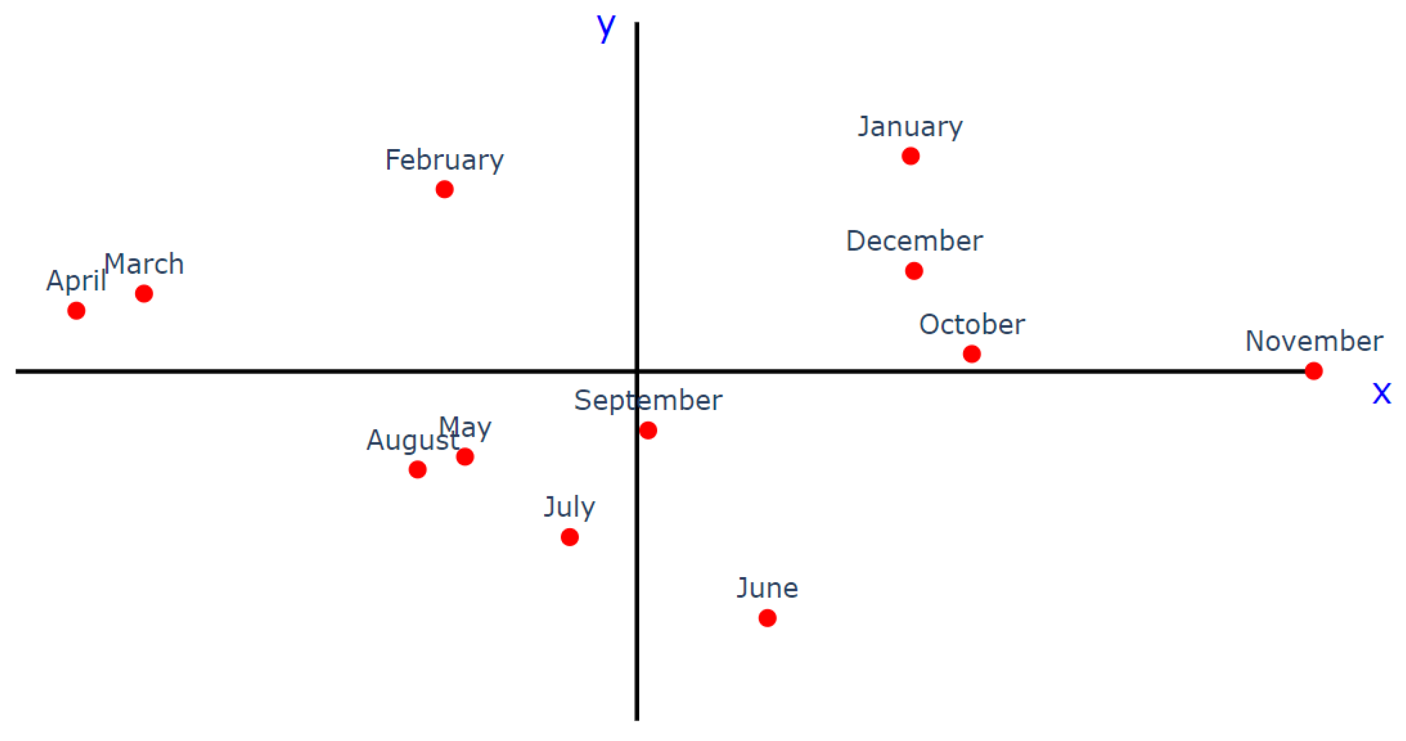
  • Month: The categorical variable m o n t h takes values in 1 12 , its dimension is three.
The dimension of the vector embeddings was fixed in accordance with the recommendations by the authors of [33] for the use of embeddings in calendar variables.

5. Experimental Study

In this section, we describe the experimental study we carried out for the prediction of the NO2 concentration in the city of Erfurt. Firstly, we will refer to the data that we used as well as the source from which they were obtained; next we will show the setup of our experiments, then the results and finally, our conclusions about the results.

5.1. Data

As indicated in Figure 9, two sets of data were needed: the historical NO2 measurements and meteorological variables. The calendar model uses only the historical NO2 time series and the meteorological model uses the historical NO2 and the meteorological variables, a multivariate time series with 7 variables.
The basic calendar information (day of the week) was directly provided by the used programming language (Python). Additional information such as about partial holidays, public holidays and bridge days was provided as a dedicated data set (CSV file) to the model. The classification of the days is described in Appendix A.
For the time series data, an integrative approach was chosen. In the first step, external data were imported from external sources and then transformed into a unified data model. Afterwards, these data were used to train the model, using a common interface for data access. It turned out that the OGC SensorThings API [34] provides an intuitive data model and an easy-to-use interface to access time-series data. In this case study, we relied on historical NO2 values from the European Environment Agency. This dataset was already available through the SensorThings API (https://datacoveeu.github.io/API4INSPIRE/datanests/ad-hoc.html and https://airquality-frost.docker01.ilt-dmz.iosb.fraunhofer.de/v1.1, accessed on 10 December 2022).
In addition, commercial weather data were used to provide the meteorological variables. Those data sources were imported into FROST® (https://github.com/FraunhoferIOSB/FROST-Server, accessed on 10 December 2022), an open-source implementation of the SensorThings API. Our forecast model uses seven weather variables, which have been recommended by Bosch (Product Area Air Quality Solutions Passenger Car (PS/PAQ-PC), Robert Bosch GmbH) experts. The considered variables are the following:
  • Wind speed (km/h);
  • Wind direction (degree);
  • Precipitation (mm/h);
  • Temperature (°C);
  • Pressure (hPa);
  • Cape (J/kg);
  • Radiation (W/m 2 ).
Since all variables have a different scale, we used the Z-score normalisation, i.e., we computed ( x μ ) / σ for each value x, where μ is the mean and σ the standard deviation of the corresponding data.
Table 2 shows the time periods for each of the considered sensors, where historical data are available. As can be seen, the last three months were used as a test sample and the rest of the data (all available data) were used to train the model. The chosen approach allows decoupling of the training of the model from data provisioning. There is an abstraction for the data source-specific interfaces: zipped CSV files from the European Environment Agency’s proprietary JSON-based interface for the meteorological variables. Only a standardized SensorThings API endpoint needs to be queried when training the model. In the future, it will be possible to exchange data sources (e.g., choosing a different provider for the meteorological variables) to obtain even better prediction results. In this case, only the import needed to be adapted, whereas the model itself kept unchanged.

5.2. Parameters, Data Structure and Models Configuration
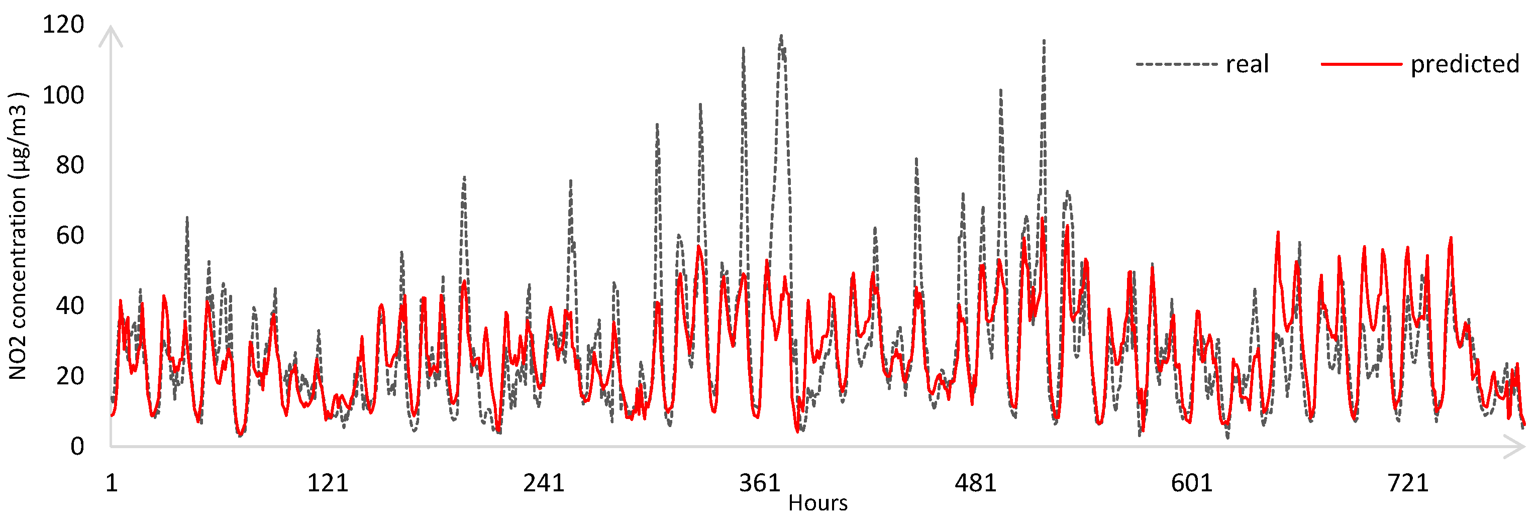
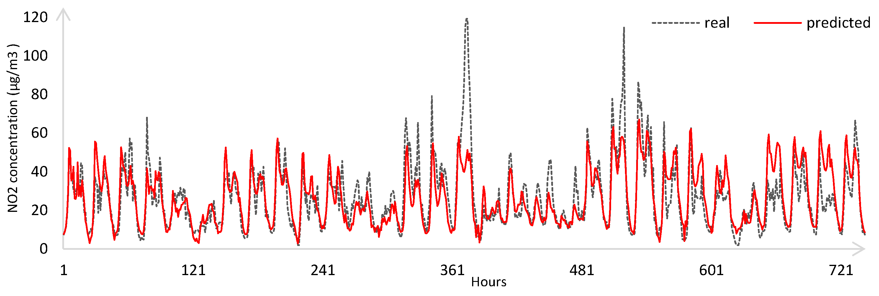
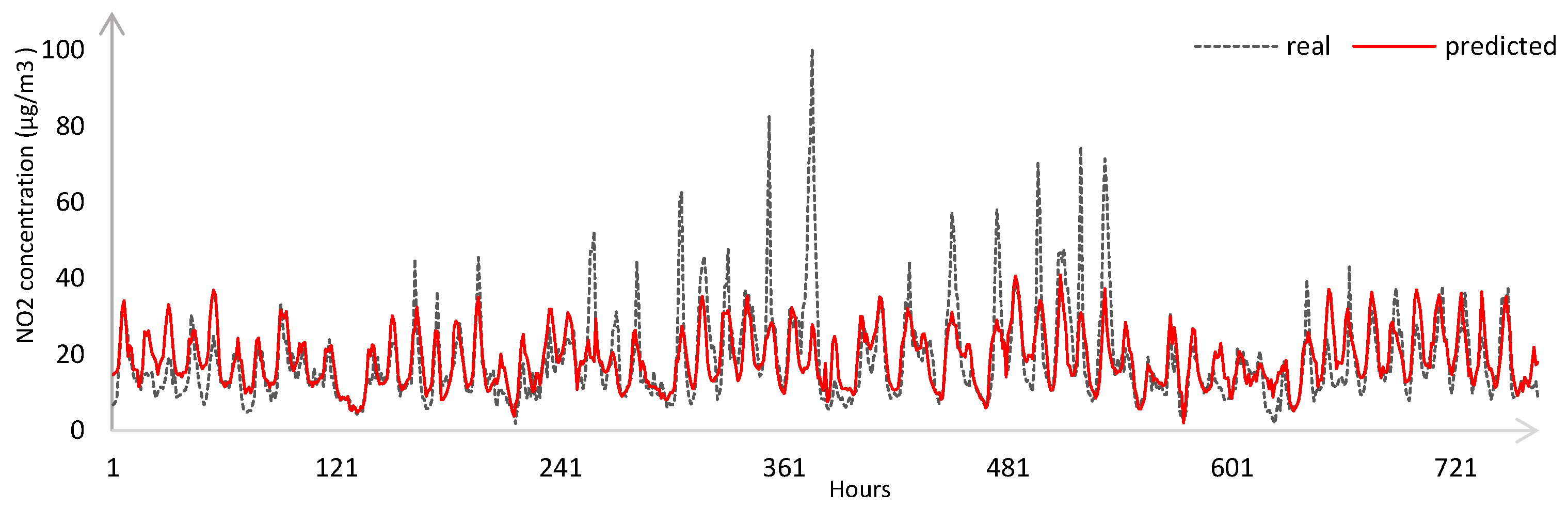
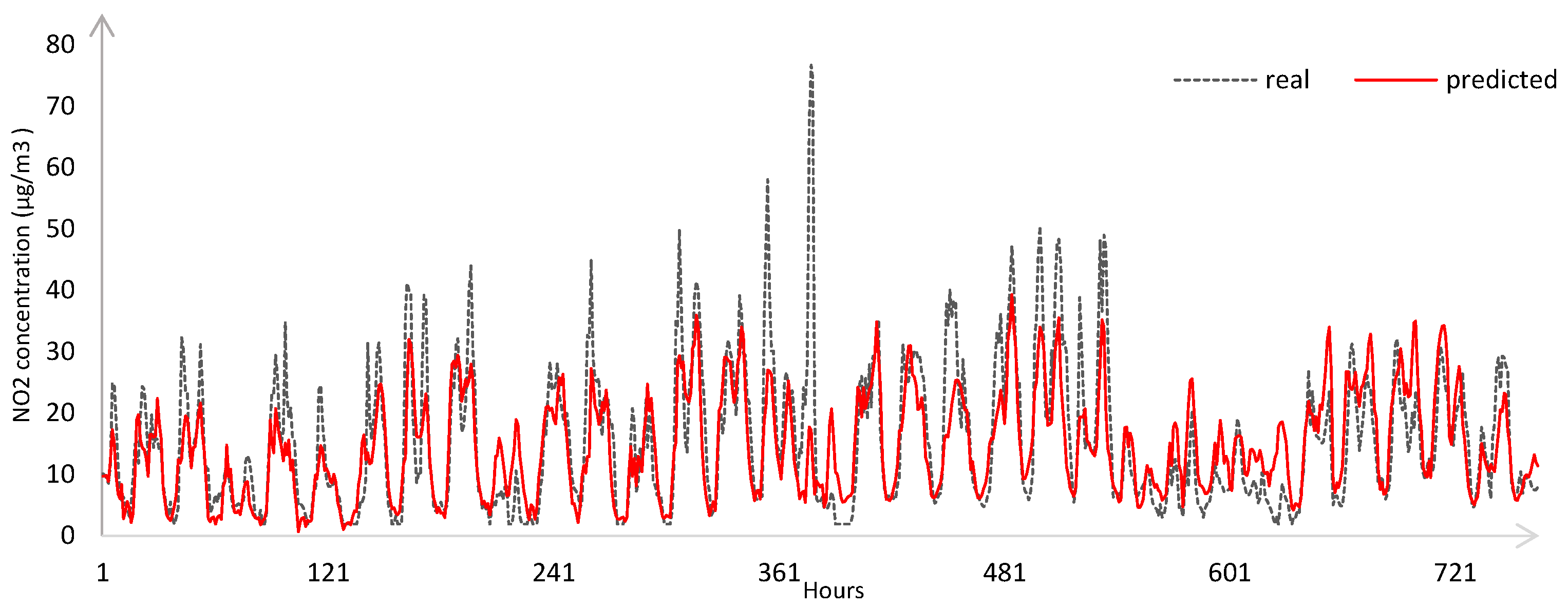
The parameters and configuration of most of the models used in the study were obtained from those recommended by the authors of the papers studied. Detailed parameters are shown in Table 3. In some cases where they were not mentioned, we used the default values, and in the case of DNN+embedding, we used those parameters recommended in [33].
Table 4 shows the configuration of the DNN+embedding used in our study. It is important to mention that for the selection of the parameters of our DNN we did not carry out any process of selection/optimisation of the hyperparameters. The selection was based on a recent study and the authors considered that, for future work, an optimisation study of the hyperparameters and the architecture of the DNN should be carried out [33].

6. Results

As we saw in the previous section, most state-of-the-art methods only predict pollutant concentrations for the next hour, which is not sufficient for our use case. Our goal was to predict 24 h of NO2 concentrations and thus make decisions that help avoid high NO2 concentrations. That is why in our experimental study we defined three time horizons:
  • Forecast the next 24 h;
  • Forecast the next 72 h;
  • Forecast the next 120 h.
As Table 2 shows, our test set is, in all cases, from September 2020 until the last day available in the data (in some cases November, in others 17 December). The training procedure followed was: starting on 1 September, we iteratively forecasted the next time horizon hours, we calculated the evaluation metric, mean absolute error (MAE Equation (1)), added the current testing period to the training set, and again we forecasted the next time horizon period. The idea behind this daily recalibration schema was to have a mean error of several testing periods (every time horizon).
M A E = 1 H i = 1 H N r N p ,
where H is the number of hours, N r is the real NO2 concentration and N p is the predicted NO2 value.
We used the standard scaler for the meteorological variables.
An important observation is that the results do not vary as the time horizon varies. This is because we used the real measurements of the meteorological variables and not the forecasts, the history of the meteorological forecast is not available in the Meteomatics API. In the final application, the model will be trained with the historical data (NO2 and meteorological variables) but the forecast of NO2 will be made from the forecast of the meteorological variables.
Table 5 shows the results of training the model with historical pollution data and meteorological variables for all the studied models. As can be seen in Table 5, the most competitive methods are model 2 of DNN+embeddings and the LGBM model used by Bosch, which significantly outperform the rest of the models.
Despite the Bosch LGBM model and model 2 using DNN+embeddings behaving very similarly, for the DETH081 sensor the difference is significant when the DNN+embedding outperforms the LGBM model by almost 1 point. In this sense, we must point out that this was what we were waiting for. As we described in Section 3 and as observed in Figure 2, sensor DETH081 is very close to a road with a lot of traffic, which makes it the sensor (of the four studied) most affected by traffic.
These results confirm our theory that, for those sensors that cover areas highly affected by traffic, the use of embedding variables to encode the calendar information in a dense neural network is a significantly superior solution to the rest of the methods with which we have compared it in this study.
In order to offer more details about the performance of our models, below we will present some plots, where it is possible to see how our model is able to predict (quite accurately) the month of September 2019, a month in which quite unusual behaviour of NO2 concentrations was observed.
In Figure 10, Figure 11, Figure 12 and Figure 13, we show the real and predicted values for the month of September 2019. The time horizon used in the prediction was 120 h (5 days). As can be seen, despite the fact that our model has a fairly accurate behaviour in the prediction, there are some peaks in which our prediction is very far from the real value. Looking in detail at those peaks, and comparing them with similar days, we discover that these values are exceedingly high and outliers. Something out of the ordinary (not meteorological) could cause this increase in the NO2 level. From our research, we know that traffic and meteorologic conditions are the main causes of variations in the levels of NO2, leading us to the assumption that an increase in traffic may be the cause of these high levels of NO2.
However, we have drawn an important conclusion from this unusual behaviour: for future improvements of our model, it would be very beneficial to have a new input variable, related to local festivities (carnivals, concerts, festivals), as well as accidents that occurred in the neighbourhood of the sensor, for the model. Although it is obvious that accidents are not predictable, and therefore this variable could not be used as input to the model to make future predictions, it could be used to explain unusual peaks.
Despite the four studied sensors registering the high outliers, sensors DETH043 and DETH081 reached the highest values, with almost 120 μ g m 3 , and sensor DETH117 (the one located in the rural area) registering the lowest peaks.

6.1. Interpretability through the Embedding Space

The embedding vectors resulting from neural network training are often very useful for finding behaviour patterns in categorical variables that cannot be distinguished with the naked eye. Following this assumption, we show the use of the embedding vector obtained during the training of the DNN to graphically understand how the models use the calendar information in the forecast. To visualise the resulting embedding vectors, we coded some functions that recreated what Tensorflow Projector does https://projector.tensorflow.org/, accessed on 10 December 2022).
Figure 14 shows in three dimensions the resulting embedding vectors for the 24 h. As can be seen, the hours form a cycle, but they do not behave like a clock.
In Figure 15 we show the projection of the resulting embeddings vectors for the dimension “day of the week”. In this case, the way in which the embedding vectors have been grouped is very interesting. Sundays and holidays are very close as well as Saturdays and bridge days; the weekdays have also created two well-defined groups, which makes total sense and is in total correspondence with what was observed in the study carried out in Section 3.
Finally, Figure 16 shows the projection of the embeddings obtained for the months of the year. In this case, although not all the months belong to well-defined groups, it can be seen, for example, that the winter months are quite close together, although partially mixed with the autumn months. Something similar happens with the spring and summer months.
As has been observed in the projection of the embeddings resulting from the training of our dense neural network, the use of embeddings not only guarantees a better encoding of the categorical variables within the neural networks but also gives us some clues about the interpretability of the results. The grouping of the categories observed in Figure 14, Figure 15 and Figure 16 can help users of our model to understand, for example, a very low forecast for a Wednesday (day of very high NO2 levels) only if that Wednesday is a holiday. It can also be useful in making decisions related to reducing NO2 levels.

6.2. Our Contribution to the Sustainable Development Goals

The Sustainable Development Goals (SDGs), also known as the Global Goals, were adopted by the United Nations (UN) in 2015 as a universal call to action to end poverty, protect the planet, and ensure that by 2030 all people enjoy peace and prosperity [35].
The 17 SDGs enunciated by the UN have become a priority for many countries, and in this sense Germany is a leader within them. Of the 17 goals stated by the UN, we believe that our work contributes to three of them (highlighted below):
  • No poverty;
  • Zero hunger;
  • Goodhealthandwell-being;
  • Quality education;
  • Gender equality;
  • Clean water and sanitation;
  • Affordable and clean energy;
  • Decent work and economic growth;
  • Industry, innovation and infrastructure;
  • Reduced inequalities;
  • Sustainablecitiesandcommunities;
  • Responsibleconsumptionandproduction;
  • Climateaction;
  • Life below water;
  • Life and land;
  • Peace, justice and strong institution;
  • Partnerships for the goals.
Goodhealthandwell-being: The reasonable, controlled and environmentally committed use of transportation, as well as the measures taken by local governments after knowing the forecast of pollutants in the air, will undoubtedly result in big health benefits.
Sustainablecitiesandcommunities: Using an application such as the one suggested in this research can help considerably with achieving more sustainable cities. Letting the population and local governments know the quality of the air they breathe, and at the same time making them participate and be responsible for reducing polluting gases, will achieve more sustainable cities and citizens more committed to the environment.
Climateaction: From our point of view, this application puts more responsibility in the hands of citizens and local governments, telling them in a closer way, “you can do a lot for the planet”. Somehow it is a popular thought to believe that climate change is a matter for big industries and governments at very high levels and that one person cannot do anything. However, this application goes to show that if "you only use your bicycle” or “take public transport” (that the government has reduced the price of), you will be able to breathe cleaner air; then, indeed, we are all taking action against climate change and taking care of the planet.

7. Conclusions and Future Work

In this paper, we have presented a study to forecast NO2 concentrations in the city of Erfurt, Germany, 1, 3 and 5 days in advance. We used some of the most significant methods within the state-of-the-art to forecast pollutants. We also introduce the use of DNN using embedding variables to encode calendar information. The comparative study carried out shows the most competitive methods the LGBM model with the hyperparameters currently used by the “Robert Bosch GmbH” and our proposal.
Although for three of the four sensors studied, there is no difference regarding the Bosch LGBM model and ours, for one of the sensors (the one that is very close to a highway with a lot of traffic) this difference is significantly in favour of our model. This result corroborates our hypothesis and allows us to conclude that, in the forecast of the NO2 concentration time series, the use of embedding variables to encode the calendar information, in a dense neural network, also encodes the traffic behaviour in a very efficient way. For this reason, we highly recommend our proposal for all those pollutants forecast applications (associated with traffic), in which the traffic data are unknown, as in our case. The second important conclusion that we can draw from our study is that the visualisation of the embedding vectors resulting from the training of the DNN can be considered a very useful tool for finding relationships between categorical variables and associated concepts, and for making decisions that in some way contribute to the reduction of emissions. In future work, we intend to improve our model by using the calendar service currently being developed by the Fraunhofer-IOSB, incorporating new meteorological variables, and optimising the DNN hyperparameters as well as the network architecture.
We like to believe that, in a very modest way, the use of our models by users at different levels (from high government officials with decision-making power to citizens who can decide whether to use a bicycle or a car) will contribute to reducing emissions of NO2.

Author Contributions

Conceptualization, E.R., S.G. and A.W.; Methodology, E.R., S.G. and A.W.; Software, E.R. and M.S.; Validation, E.R. and M.S.; Formal analysis, E.R. and S.G.; Investigation, E.R., S.G., M.S. and A.W.; Writing—original draft, E.R., S.G., M.S. and A.W.; Writing—review & editing, E.R., S.G., M.S. and A.W.; Visualization, E.R.; Supervision, A.W.; Project administration, S.G. All authors have read and agreed to the published version of the manuscript.

Funding

This research was funded by Federal Ministry for Economic Affairs and Energy, granted number 01MK20013A.

Institutional Review Board Statement

Not applicable.

Informed Consent Statement

Not applicable.

Data Availability Statement

Not applicable.

Acknowledgments

This research was funded by the Bundesministerium für Wirtschaft und Energie (BMWi) grant number 01MK20013A. The authors would like to thank Gabriel Braun and the Product Area Air Quality Solutions Passenger Car (PS/PAQ-PC) Robert Bosch GmbH for their valuable help. We are also immensely grateful to Bauhaus.MobilityLab for building up a fruitful research environment. Many thanks to our colleague Hylke van der Schaaf for supporting us with his expert knowledge of the SensorThings API. Many thanks also to our colleague Tania Jacob for her valuable revision.

Conflicts of Interest

The authors declare no conflict of interest.

Appendix A. Detailed Classification of Public Holidays

The embedding for calendar features builds upon the following classification of holidays:
  • public holidays: Christmas, Day After Christmas, New Years Day, First of May (International Workers Day), Day of German Unity, Good Friday, Easter Sunday, Easter Monday, Ascension Day, Pentecost Monday,
  • partial holidays: assumption of Mary, Reformation Day, All Hallows Day, Day of Prayer and Repentance, Pentecost Sunday, the Christmas week,
  • bridge days: all days between public holidays, Fridays if Thursdays are public holidays and Mondays if Tuesdays are public holidays.

References

  1. Saki, H.; Mohammadi, G. Estimation of health effect attributed to NO2 exposure by using of Air Q model in Ahwaz, 2009. Apadana J. Clin. Res. 2013, 2, 5–12. [Google Scholar]
  2. Dons, E.; Laeremans, M.; Anaya-Boig, E.; Avila-Palencia, I.; Brand, C.; de Nazelle, A.; Gaupp-Berghausen, M.; Götschi, T.; Nieuwenhuijsen, M.; Orjuela, J.P.; et al. Concern over health effects of air pollution is associated to NO2 in seven European cities. Air Qual. Atmos. Health 2018, 11, 591–599. [Google Scholar] [CrossRef]
  3. Zhao, S.; Liu, S.; Sun, Y.; Liu, Y.; Beazley, R.; Hou, X. Assessing NO2-related health effects by non-linear and linear methods on a national level. Sci. Total. Environ. 2020, 744, 140909. [Google Scholar] [CrossRef] [PubMed]
  4. Hesterberg, T.W.; Bunn, W.B.; McClellan, R.O.; Hamade, A.K.; Long, C.M.; Valberg, P.A. Critical review of the human data on short-term nitrogen dioxide (NO2) exposures: Evidence for NO2 no-effect levels. Crit. Rev. Toxicol. 2009, 39, 743–781. [Google Scholar] [CrossRef]
  5. Snowden, J.M.; Mortimer, K.M.; Kang Dufour, M.S.; Tager, I.B. Population intervention models to estimate ambient NO2 health effects in children with asthma. J. Expo. Sci. Environ. Epidemiol. 2015, 25, 567–573. [Google Scholar] [CrossRef]
  6. Statista. Per capita nitrogen oxide (NOx) emissions in 2020, by select country. 2022. Available online: https://www.statista.com/statistics/478834/leading-countries-based-on-per-capita-nitrogen-oxide-emissions/ (accessed on 1 February 2023).
  7. Zhou, R.; Wang, S.; Shi, C.; Wang, W.; Zhao, H.; Liu, R.; Chen, L.; Zhou, B. Study on the Traffic Air Pollution inside and outside a Road Tunnel in Shanghai, China. PLoS ONE 2014, 9, e112195. [Google Scholar] [CrossRef]
  8. Zhang, L.; Guan, Y.; Leaderer, B.; Holford, T. Estimating daily nitrogen dioxide level: Exploring traffic effects. Ann. Appl. Stat. 2013, 7, 1763–1777. [Google Scholar] [CrossRef]
  9. Agency, E.E. Impact of Selected Policy Measures on Europe’s AIR Quality. 2015. Available online: https://www.eea.europa.eu/data-and-maps/daviz/sector-share-of-nitrogen-oxides-emissions/ (accessed on 1 February 2023).
  10. Flämig, P.D.I.H. Luft- und Klimabelastung Durch Güterverkehr. 2021. Available online: https://www.forschungsinformationssystem.de/servlet/is/39787/ (accessed on 1 February 2023).
  11. Reddy, V.; Yedavalli, P.; Mohanty, S.; Nakhat, U. Deep air: Forecasting air pollution in Beijing, China. Environ. Sci. 2018, 1564. [Google Scholar]
  12. Tao, Q.; Liu, F.; Li, Y.; Sidorov, D. Air Pollution Forecasting Using a Deep Learning Model Based on 1D Convnets and Bidirectional GRU. IEEE Access 2019, 7, 76690–76698. [Google Scholar] [CrossRef]
  13. Liang, Y.C.; Maimury, Y.; Chen, A.; Juarez, J. Machine Learning-Based Prediction of Air Quality. Appl. Sci. 2020, 10, 9151. [Google Scholar] [CrossRef]
  14. Kleine Deters, J.; Zalakeviciute, R.; Gonzalez, M.; Rybarczyk, Y. Modeling PM 2.5 Urban Pollution Using Machine Learning and Selected Meteorological Parameters. J. Electr. Comput. Eng. 2017, 2017, 5106045. [Google Scholar] [CrossRef]
  15. Behm, S.; Haupt, H.; Schmid, A. Spatial detrending revisited: Modelling local trend patterns in NO2 concentration in Belgium and Germany. Spat. Stat. 2018, 28, 331–351. [Google Scholar] [CrossRef]
  16. Donnelly, A.; Naughton, O.; Broderick, B.; Misstear, B. Short-Term Forecasting of Nitrogen Dioxide (NO2) Levels Using a Hybrid Statistical and Air Mass History Modelling Approach. Environ. Model. Assess. 2017, 22, 231–241. [Google Scholar] [CrossRef]
  17. Samal, K.K.R.; Babu, K.S.; Das, S.K.; Acharaya, A. Time series based air pollution forecasting using SARIMA and prophet model. In Proceedings of the 2019 International Conference on Information Technology and Computer Communications, Singapore, 16–18 August 2019; pp. 80–85. [Google Scholar]
  18. Qadeer, K.; Jeon, M. Prediction of PM10 Concentration in South Korea Using Gradient Tree Boosting Models. In Proceedings of the 3rd International Conference on Vision, Image and Signal Processing, Vancouver, BC, Canada, 26–28 August 2019; Association for Computing Machinery: New York, NY, USA, 2019. [Google Scholar] [CrossRef]
  19. Qadeer, K.; Rehman, W.U.; Sheri, A.; Park, I.; Kim, H.; Jeon, M. A Long Short-Term Memory (LSTM) Network for Hourly Estimation of PM2.5 Concentration in Two Cities of South Korea. Appl. Sci. 2020, 10, 3984. [Google Scholar] [CrossRef]
  20. Li, Z.; Yim, S.H.L.; Ho, K.F. High temporal resolution prediction of street-level PM2.5 and NOx concentrations using machine learning approach. J. Clean. Prod. 2020, 268, 121975. [Google Scholar] [CrossRef]
  21. Iskandaryan, D.; Ramos, F.; Trilles, S. Bidirectional convolutional LSTM for the prediction of nitrogen dioxide in the city of Madrid. PLoS ONE 2022, 17, e0269295. [Google Scholar] [CrossRef] [PubMed]
  22. Dairi, A.; Harrou, F.; Khadraoui, S.; Sun, Y. Integrated multiple directed attention-based deep learning for improved air pollution forecasting. IEEE Trans. Instrum. Meas. 2021, 70, 1–15. [Google Scholar] [CrossRef]
  23. Al-Janabi, S.; Alkaim, A.; Al-Janabi, E.; Aljeboree, A.; Mustafa, M. Intelligent forecaster of concentrations (PM2.5, PM10, NO2, CO, O3, SO2) caused air pollution (IFCsAP). Neural Comput. Appl. 2021, 33, 14199–14229. [Google Scholar] [CrossRef]
  24. Casquero-Vera, J.A.; Lyamani, H.; Titos, G.; Borrás, E.; Olmo, F.; Alados-Arboledas, L. Impact of primary NO2 emissions at different urban sites exceeding the European NO2 standard limit. Sci. Total Environ. 2019, 646, 1117–1125. [Google Scholar] [CrossRef]
  25. Kurtenbach, R.; Kleffmann, J.; Niedojadlo, A.; Wiesen, P. Primary NO2 emissions and their impact on air quality in traffic environments in Germany. Environ. Sci. Eur. 2012, 24, 21. [Google Scholar] [CrossRef]
  26. Kamińska, J.A. A random forest partition model for predicting NO2 concentrations from traffic flow and meteorological conditions. Sci. Total Environ. 2019, 651, 475–483. [Google Scholar] [CrossRef] [PubMed]
  27. Jiménez-Hornero, F.; Jimenez-Hornero, J.; Gutiérrez de Ravé, E.; Pavón-Domínguez, P. Exploring the relationship between nitrogen dioxide and ground-level ozone by applying the joint multifractal analysis. Environ. Monit. Assess. 2009, 167, 675–684. [Google Scholar] [CrossRef]
  28. McCulloch, W.S.; Pitts, W. A logical calculus of the ideas immanent in nervous activity. Bull. Math. Biophys. 1943, 5, 115–133. [Google Scholar] [CrossRef]
  29. Hopfield, J. Neural Networks and Physical Systems with Emergent Collective Computational Abilities. Proc. Natl. Acad. Sci. USA 1982, 79, 2554–2558. [Google Scholar] [CrossRef] [PubMed]
  30. Hinton, G.E.; Osindero, S.; Teh, Y.W. A Fast Learning Algorithm for Deep Belief Nets. Neural Comput. 2006, 18, 1527–1554. [Google Scholar] [CrossRef] [PubMed]
  31. Bengio, Y.; Ducharme, R.; Vincent, P.; Jauvin, C. A Neural Probabilistic Language Model. J. Mach. Learn. Res. 2003, 3, 1137–1155. [Google Scholar]
  32. Cartuyvels, R.; Spinks, G.; Moens, M.F. Discrete and continuous representations and processing in deep learning: Looking forward. AI Open 2021, 2, 143–159. [Google Scholar] [CrossRef]
  33. Wagner, A.; Ramentol, E.; Schirra, F.; Michaeli, H. Short- and long-term forecasting of electricity prices using embedding of calendar information in neural networks. J. Commod. Mark. 2022, 28, 100246. [Google Scholar] [CrossRef]
  34. Liang, S.; Huang, C.; Khalafbeigi, T. OGC SensorThings API Part 1: Sensing, Version 1.0; Open Geospatial Consortium: Wayland, MA, USA, 2016. [Google Scholar]
  35. The Sustainable Development Goals. Available online: https://www.undp.org/sustainable-development-goals (accessed on 19 January 2023).
Figure 1. Main sources of NO2 emissions of nitrogen oxides. (a) Contribution made by different sectors to emissions of nitrogen oxides in 2011. (b) Different emission sources in traffic 2017, Germany.
Atmosphere 14 00298 g001
Figure 2. Location of the sensors in the city of Erfurt.
Atmosphere 14 00298 g002
Figure 3. Box plots for the four sensors.
Atmosphere 14 00298 g003
Figure 4. NO2 concentration for the four sensors, first two weeks of September 2020.
Atmosphere 14 00298 g004
Figure 5. NO2 concentration for rural sensors, September 2020, first two weeks sensors.
Atmosphere 14 00298 g005
Figure 6. NO2 concentration for urban sensors, September 2020, first two weeks sensors.
Atmosphere 14 00298 g006
Figure 7. Weekly seasonality NO2 concentration for the four sensors (DETH020 blue, DETH043 violet, DETH081 red, DETH117 green), week from 9 November until 15 November 2020.
Atmosphere 14 00298 g007
Figure 8. NO2 concentration for three sensors, from October 1 until 5 October 2018.
Atmosphere 14 00298 g008
Figure 9. General scheme for DNN with an embedding layer.
Atmosphere 14 00298 g009
Figure 10. Real and predicted NO2, Sensor DETH043, September 2019, horizon: 120 h.
Atmosphere 14 00298 g010
Figure 11. Real and predicted NO2, Sensor DETH081, September 2019, horizon: 120 h.
Atmosphere 14 00298 g011
Figure 12. Real and predicted NO2, Sensor DETH020, September 2019, horizon: 120 h.
Atmosphere 14 00298 g012
Figure 13. Real and predicted NO2, Sensor DETH117, September 2019, horizon: 120 h.
Atmosphere 14 00298 g013
Figure 14. Hours in the embedding space.
Atmosphere 14 00298 g014
Figure 15. Weekdays in the embedding space.
Atmosphere 14 00298 g015
Figure 16. Month in the embedding space.
Atmosphere 14 00298 g016
Table 1. State-of-the-art literature overview.
PaperAlgorithmHorizonComparedData
[16]Hybrid statistical24 h-Irish EPA
[11]LSTM encoder-decoder5 h, 10 h, 120 hLSTM, sequence-to-scalarBeijing
[12]1D CNN-GRU a 1 hSVR b , DTR c , LSTM, BGRU d UCI-repo
[17]Prophet1 hBox-JenkinBhubaneshwar
[14]ANN e-BT f , LSVM g Belisario, Cotocollao
[13]Adaboost1 h, 8 h, 24 hSVM, ANN, Random ForestTaiwan EPA
[18]LGBM-XGB h , LGBMSouth Korea
[19]LSTM1 hXGB, LGBM, LSTMSouth Korea
[20]Random Forest-BRT i , SVM, XGB, GAM j , CubistHong Kong
[21]BC-LSTM k 6 hC-LSTM, LSTMMadrid
[22]IMDA-VAE l -GRU, BGRU, LSTM, VAE, C-LSTM, B-LSTMArizona, California, Pennsylvania, Texas
[23]DLSTM m 48 hLSTMChina
a 1-D deep convolutional gated recurrent neural network, b support vector regression, c dynamic treatment regime, d bidirectional GRU, e Artificial neural networks, f boosted trees, g linear support vector machine, h extreme gradient boosting, i boosted regression trees, j generalized additive model, k bidirectional convolutional LSTM, l integrated multiple directed attention variational autoencoder, m developed LSTM.
Table 2. Training and testing period per sensor.
SensorData PointsTrainingTesting
DETH043169592018, 2019, 2020 until AugustSeptember, October and November 2020
DETH020251272018, 2019, 2020 until AugustSeptember, October and November 2020
DETH117159672019, 2020 until AugustSeptember, October and November 2020
DETH081150102019, 2020 until AugustSeptember, October and November 2020
Table 3. Parameter and model configuration for methods used in our study.
ModelParametersInput Data
DNNTable 4model 1: calendar
model 2: cal+met
LSTMhidden layer = 2cal+met
neurons/layer = 64
epochs = 30
dropout = 0.4
optimizer = Adam
loss = MSE
LGBM_Bosh parametermax_depth: −1cal+met
learning_rate: 0.005
num_iterations: 4837
feature_fraction:0.6
bagging_fraction: 0.9
bagging_freq: 5
LGBM_bayesian_optmax_depth: 15cal+met
min_split_gain: 0.1
num_iterations: 100
feature_fraction:1.0
bagging_fraction:1.0
num_leaves:5
LGBM_Qadeermax_depth:-1cal+met
learning_rate:0.005
num_iterations: 4837
feature_fraction:0.6
bagging_fraction:0.9
bagging_freq:5
Adaboostbase_estimator = Decision_treecal+met
n_estimator = 50
learning_rate = 1.0
LSTM-encoder-decoderdropout = 0.4cal+met
loss = MSE
epochs =30
optimizer = Adam
encoder_LSTM
embedding layer = 1
embedding layer neurons = 16
encoder_rnn_hidden = 224
decoder_LSTM
embedding layer = 1
embedding layer neurons = 16
decoder_rnn_hidden = 224
cal+met: calendar variables and meteorological variables forecasting.
Table 4. Dense neural network parameters.
ParametersDNN
ModelSequential
Hidden layers2
Neurons per layer60/60/1
Loss functionmse
Type of layerdense
Activation outputlinear
Activation hidden layersrelu/relu
Epoch100
OptimizerRMSprop(0.001)
Table 5. Mean absolute error average for all the compared methods.
SensorMethodData/Encode24 h72 h120 h
DE_DETH043DNN+embeddingmodel 19.19299.12489.3957
model 27.17007.38587.4489
LGBMordinal7.23257.32167.4517
one_hot7.27897.42977.4600
LGBM-BOSCHordinal6.94207.08377.1495
LSTMinput = 108.77438.40078.1686
input = 2410.710911.232710.8840
Adaboostonehot13.279613.350313.1704
ordinal12.564412.340612.5564
LSTM-AEseq len 511.024914.076814.3268
DE_DETH020DNN+embeddingmodel 16.56896.75916.8499
model 24.95595.10954.9550
LGBMordinal5.29475.28845.3362
one_hot5.38565.41015.3858
LGBM-BOSCHordinal5.10395.16415.2147
LSTMinput = 105.33485.37185.4127
input = 246.40976.50726.2651
Adaboostonehot8.23448.09557.9516
ordinal9.30919.14179.3261
LSTM-AEseq len 57.99559.30039.4265
DE_DETH117DNN+embeddingmodel 16.67086.60766.7113
model 24.39124.50714.4123
LGBMordinal4.30284.37224.4029
one_hot4.33914.42804.4166
LGBM-BOSCHordinal4.18094.29064.2971
LSTMinput = 104.62094.77254.8600
input = 245.95995.88416.0775
Adaboostonehot7.46507.46337.5334
ordinal7.46517.30917.2455
LSTM-AEseq len 57.41137.79737.7239
DE_DETH081DNN+embeddingmodel 17.58898.00228.1991
model 26.43816.39696.8792
LGBMordinal7.48387.72987.9176
one_hot7.39267.53207.7081
LGBM-BOSCHordinal7.28727.50837.5210
LSTMinput = 108.28267.90867.7629
input = 2411.391511.550611.3960
Adaboostonehot13.396813.541213.4224
ordinal13.518613.683613.1394
LSTM-AEseq len 510.809615.022314.6538
Disclaimer/Publisher’s Note: The statements, opinions and data contained in all publications are solely those of the individual author(s) and contributor(s) and not of MDPI and/or the editor(s). MDPI and/or the editor(s) disclaim responsibility for any injury to people or property resulting from any ideas, methods, instructions or products referred to in the content.

