Prediction of Aircraft Go-Around during Wind Shear Using the Dynamic Ensemble Selection Framework and Pilot Reports

Abstract

Pilots typically implement the go-around protocol to avoid landings that are hazardous due to wind shear, runway excursions, or unstable approaches. Despite its rarity, it is essential for safety. First, in this study, we present three Dynamic Ensemble Selection (DES) frameworks: Meta-Learning for Dynamic Ensemble Selection (META-DES), Dynamic Ensemble Selection Performance (DES-P), and K-Nearest Oracle Elimination (KNORAE), with homogeneous and heterogeneous pools of machine learning classifiers as base estimators for the prediction of aircraft go-around in wind shear (WS) events. When generating a prediction, the DES approach automatically selects the subset of machine learning classifiers which is most probable to perform well for each new test instance to be classified, thereby making it more effective and adaptable. In terms of Precision (86%), Recall (83%), and F1-Score (84%), the META-DES model employing a pool of Random Forest (RF) classifiers outperforms other models. Environmental and situational factors are subsequently assessed using SHapley Additive exPlanations (SHAP). The wind shear magnitude, corridor, time of day, and WS altitude had the greatest effect on SHAP estimation. When a strong tailwind was present at low altitude, runways 07R and 07C were highly susceptible to go-arounds. The proposed META-DES with a pool of RF classifiers and SHAP for predicting aircraft go-around in WS events may be of interest to researchers in the field of air traffic safety.

1. Introduction

An abrupt change in wind direction or speed of at least 14 knots and below 1600 feet (500 m) above runway level is referred to as wind shear (WS) in the aviation industry [1]. This could be the result of environmental conditions such as a thunderstorm, gust, or sea breeze, or it could be the result of the airport’s proximity to complex terrain, such as mountains or man-made structures. The occurrence of wind shear is regarded as one of the most dangerous phenomena for approaching and departing aircrafts [2].

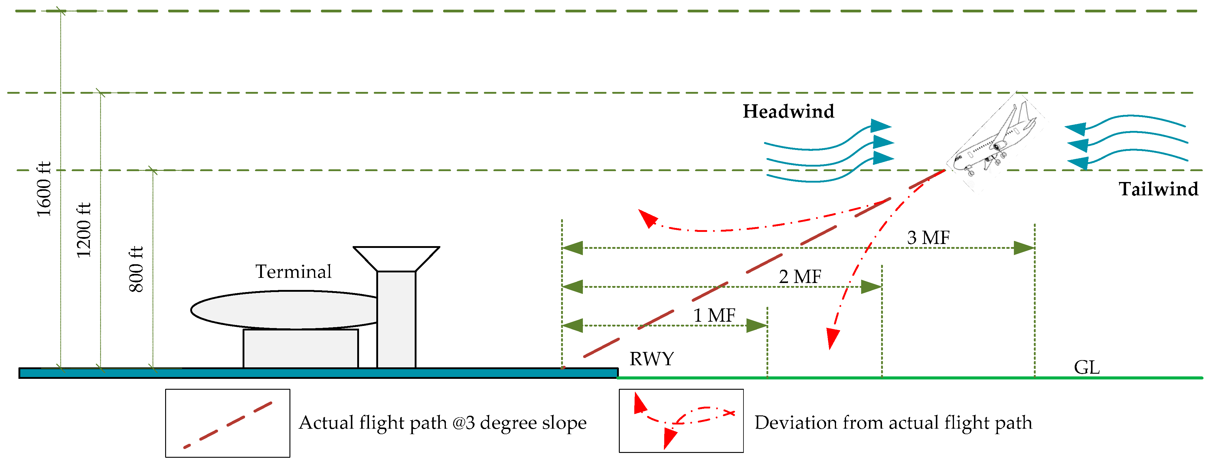
During the landing phase, the flight deck remains highly engaged, and the pilots must make a number of split-second decisions to complete their landing checklist. However, adverse weather conditions such as wind shear, mountainous terrain, and the presence of buildings close to the airport could increase turbulence along the glide path. While completing the landing checklist, the pilot must contend with violent updrafts and downdrafts and abrupt changes in the aircraft’s horizontal and vertical movement. As shown in Figure 1, the head wind shear or tail wind shear may result in landing short of the runway (loss of lift) or deviating from the actual flight path during the final approach. Consequently, pilots initiate a go-around procedure. Despite that this protocol is implemented to prevent unsafe landings, their complicated maneuvering procedures and limited available time can raise additional safety concerns, particularly in wind shear events. As a result of this operational anomaly, air traffic controllers have a greater workload, and noise levels have massively increased [3,4]. Additionally, the airport throughput and punctuality of flights are negatively impacted [5,6]. Majority of go-arounds are performed at low altitudes and low speeds, necessitating immediate adjustments to the aircraft’s altitude, thrust, and flight path to avoid collisions with nearby air traffic.

Since wind shear plays a major role in the execution of go-around protocols, airports around the world have benefited greatly from the availability of precise remote sensing technologies, including Terminal Doppler Weather Radar (TDWR) and Doppler Light Detection and Range (LiDAR), to timely detect WS events [7,8,9]. Researchers in the past have used a wide range of approaches to predict go-around based on various parameters as well as contributing factors, including the environment, such as wind speed, visibility, and pressure, etc., unstable approach and a change in runway configuration, as well as physiological conditions associated with the pilot and air traffic controller, as shown in

Table 1. Literature on various factors contributing to the occurrence of aircraft go-around.

Serial No.	Parameters	Contributing Factors	Model Employed	Literature
1.	Environment	Visibility, wind speed, and localizer deviation significantly impacted go-around.	Flight simulation of Airbus A330-200 and Boeing 737-800	[10]
		Visibility, wind speed, and pressure significantly impacted go-around.	Categorical Boosting	[11]
		Thunderstorms and winds exceeding 29 mph significantly impacted go-around	Statistical model	[12]
2.	Pilot and air traffic controller	Unpleasant psychological condition compromised pilot decision-making and cognitive performance that resulted in go-around	Neuro-economics brain imaging protocol	[13]
		Anomalies in pilot flying performance, including flight path deviations and visual scanning behaviors caused go-around	Flight simulator test	[14]
		Situational unawareness by air traffic controllers caused go-around	Path analysis and bootstrap	[15]
		Age and experience of air traffic controllers contributed to go-around	Flight simulator test	[16]
		Pilot and controller experiences and mental states	Surveys and interviews	[6]
3.	Unstable approach/runway configuration	Quantification of aircraft deviation at final approach	Sparse Variation Gaussian process	[17]
		Approach stability, departure air traffic, flight spacing, departure traffic, and ceiling contributed to go-around	Principal component analysis	[18]

.

While these studies have shed light on the many factors that can lead to a go-around, none of them have examined the role that wind shear plays in this phenomenon. There is a significant gap in the literature about the prediction of go-around under wind shear conditions. The occurrence of go-around due to wind shear is usually a rare event, however, predicting its occurrence under wind shear conditions is of utmost importance. Therefore, the goal of this research is to quantify the factors that contribute to the occurrence of go-around triggered by wind shear and situational factors, such as time of day, season of the year, and flight and aircraft type. In this study, our study location is Hong Kong International Airport (HKIA) and we used HKIA-based pilot report (PIREPs) data. We then employed dynamic ensemble learning strategies to classify go-around and approaches of aircrafts. 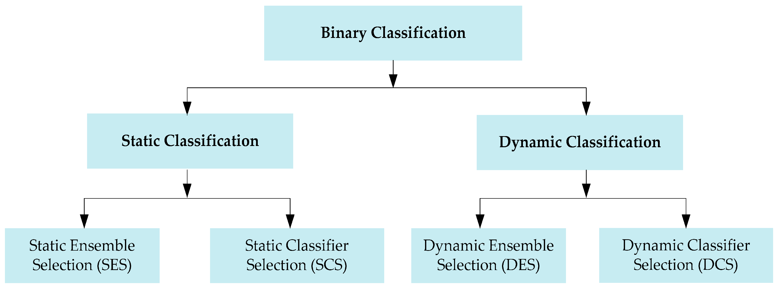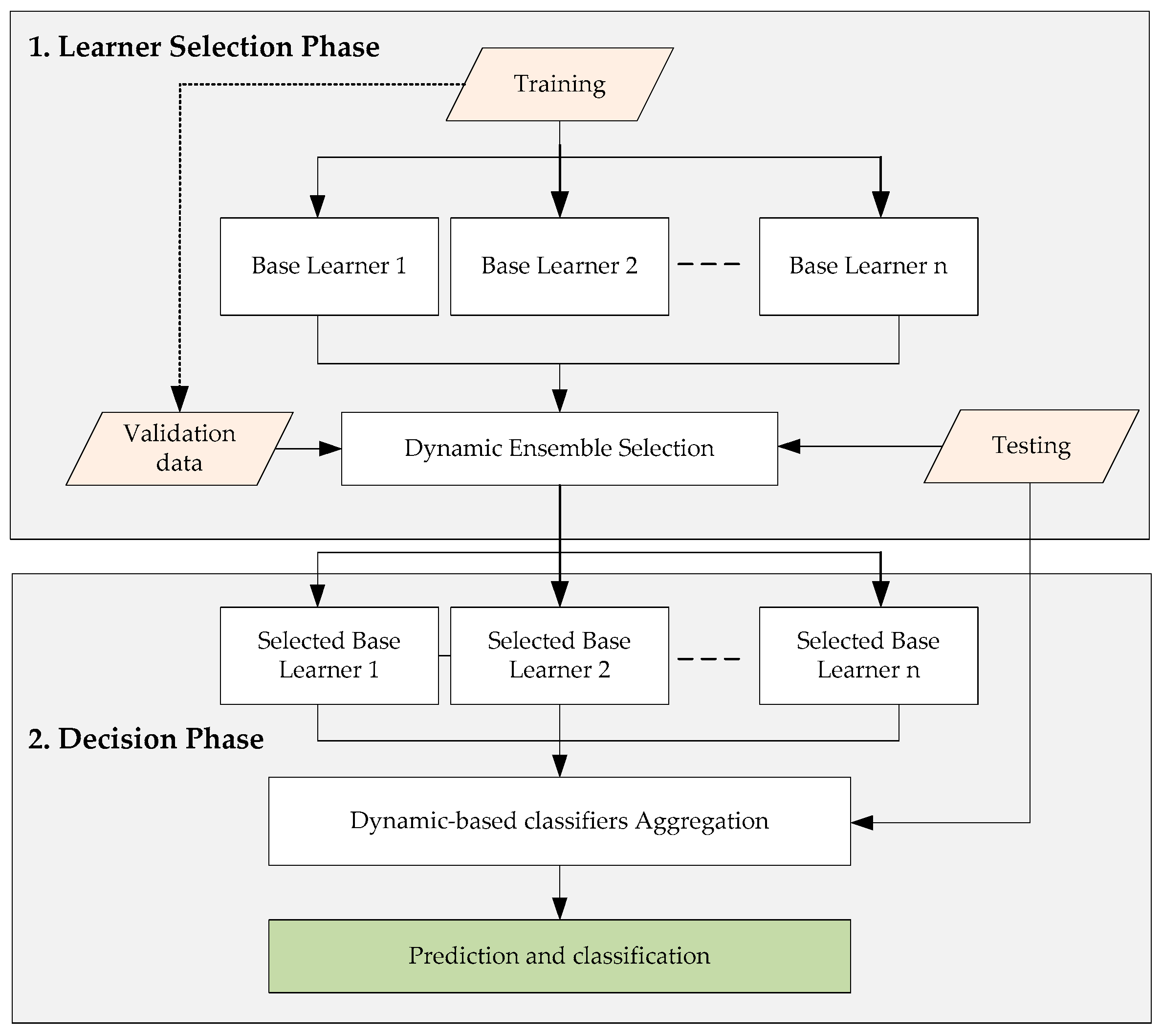In many practical situations, ensemble learning has outperformed a single machine learning approach [19,20,21,22]. Stacking, bagging, and boosting are the three main ideas of ensemble learning, which encapsulates the techniques and strategies of model blending. The fundamental aim of ensemble learning is to pool the efficacy of several classification models into a single conclusion. A dataset with many factors or characteristics for each instance constitutes a binary classification problem. One of the considerations is the decision label, which should be categorical and reveal to which group each instance belongs. The goal of classification strategies is to build classification models that can predict and classify the dependent label for the given sample. The two most common kinds of classification schemes are dynamic and static. A comparison of ensemble and classification model selection techniques for static and dynamic classification approaches is depicted in Figure 2 [23,24]. The primary difference between static and dynamic classification approaches is whether all the test samples are predicted with the same classifier. Similar to how classifier selection differs from ensemble classifier selection, a single classifier model can be comprised of several base classifiers that are employed to predict a test sample, leading to a wide number of classification techniques that rely on their unique combination. In most cases, the performance of a static classification strategy is inferior to that of a dynamic one, as various classification models excel in various settings.

For this research, we used three DES models, including Meta-Learning for Dynamic Ensemble Selection (META-DES) [25], K-Nearest Oracle Elimination (KNORAE) [26], and Dynamic Ensemble Selection Performance (DES-P) [27], whose input is the pools of homogenous and heterogeneous classification algorithms. The pools of homogenous and homogenous classification algorithms are highlighted in

Table 2. Pools of various classification algorithms for the study.

Ensemble	Pools of Algorithm	Reference
Homogenous	Random Forest (RF)	[28]
	Extremely Randomized Tree (ERT)	[29]
	Bagging Multi-Layer Perceptron (BMLP)	[30]
Heterogeneous	K-Nearest Neighbor (KNN)	[27]
	Support Vector Machine (SVM)	[31]
	Binary Logistic Regression (BLR)	[32]

. Afterward, SHAP analysis interpreted the results of the optimal DES model and illustrated important factors contributing to go-around under WS conditions.

Machine learning models are typically black boxes, so their predictions may not make the connection between input and output changes crystal clear. The interpretation of the model is equally important for an insight of the model’s performance. Factor analysis methods, such as permutation-based importance scores, were previously employed to decipher the outcomes of machine learning studies. However, the factor importance analysis can only rank the significance of the factors, and it does not comprehend how each factor affects the model’s prediction on its own. SHapley Additive exPlanations (SHAP) analysis, inspired by game theory [33], has been used in recent studies to quantitatively assess the relative importance of each contributing factor [34,35,36]. Use of SHAP with machine learning models allows for the interpretation of the relative contributions and the importance of different factors [37,38,39,40].

Our findings would aid pilots, flight attendants, air traffic controllers, and policymakers in estimating when a go-around is requisite. Second, identifying mitigation strategies to reduce aircraft go-around and, more generally, the circumstances that lend credence to them, which may be deemed anomalous and inherently unappealing, can be aided by quantifying the contributing factors of go-around occurrences. It is possible to reduce the need for go-around by implementing mitigation strategies such as adjustment of protocols, enhancing pilot education, and revamping hardware.

The remainder of this paper is structured as follows. Section 2 illustrates the research methodology and discusses our sources of data, DES models, and the SHAP interpretation strategy. Section 3 details the DES models’ performance as a comparison as well as the SHAP analysis results. Section 4 encompasses the conclusion of our study and recommendations.

2. Methodology

In this study, we first analyzed the pilot reports (PIREPs) of Hong Kong International Airport (HKIA) to determine the factors that most likely contributed to the go-around. A PIREP is an abbreviation for pilot reports used in civil aviation. The pilots who encounter hazardous weather conditions and go-around are sent to air traffic controllers. The factors that can influence go-around include weather conditions such as wind shear conditions (wind shear magnitude, altitude, and horizontal location of wind shear from the runway as well as its causes), precipitation (rainfall), aircraft and flight (wide or narrow-body aircraft, international or domestic flight), landing runway, and temporally specific factors such as the season of the year and time of the day (daytime/nighttime).

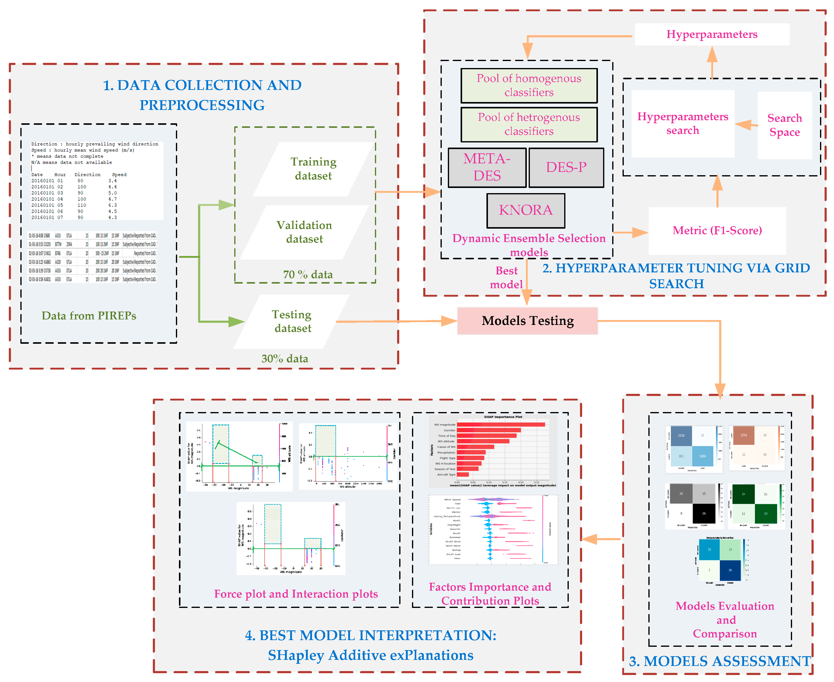
Secondly, we built DES models with different pools of homogenous and heterogeneous classifiers as base estimators to predict aircraft go-around in case of WS events. Based on the model with the best performance, lastly, we estimated the importance and contributions of various factors to go-around occurrence using the SHAP interpretation approach. Figure 3 depicts the whole operational paradigm proposed in this study.

2.1. Study Location

The HKIA is located on an artificial Lantau Island on the southeastern coast of mainland China in a subtropical zone. The tropical cyclones and southwest monsoon are two typical convective weather conditions that occur in Hong Kong. In addition to bringing thunderstorms and showers to the region, the convective weather interrupts air traffic. Due to these reasons, Hong Kong International Airport (HKIA) is among the airports most susceptible to WS in the vicinity of the runway. Numerous observational and modeling studies have shown that HKIA’s intricate orography and complex land–sea contrast are also conducive to the occurrence of WS [41]. Significant WS events occur once every 400 to 500 flights. From the opening of HKIA in 1998 until 2015, 97.70% of reports illustrated 15–25 knots of WS [42].

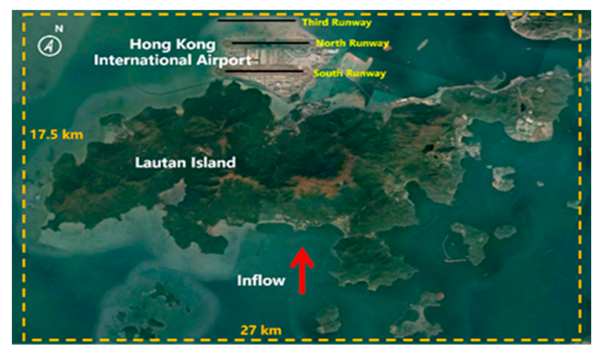
Figure 4 shows that HKIA is surrounded on three sides by open sea water and mountains to the south, which reaches elevations of over 900 m above sea level. This complex terrain surrounding HKIA also contributes to terrain-induced WS. The mountainous terrain to the south of HKIA amplifies WS, disrupting airflow and generating mountain waves, gap discharge, and other disturbances along the HKIA flight paths. Three runway corridors exist at HKIA: the North Runway (Northern Corridor), the Central Runway (Central Corridor), and the South Runway (Southern Corridor). The Northern Corridor is a newly constructed runway, and therefore the previous Northern Corridor is now designated as the Central Corridor. They are oriented in the 070° and 250° directions. Since each runway can be used for takeoffs and landings in either direction, there are a total of twelve possible configurations. For example, runway ‘07LA’ denotes landing (‘A’ refers to arrival) with a heading angle of 070° (shortened to ‘07’) using the left runway (hence ‘L’). This shows aircraft landing on the Northern Corridor from the western side of HKIA. Likewise, an aircraft departing the Southern Corridor in the west would use runway 25LD.

2.2. Data Processing from PIREPs

As stated earlier, pilot reports are abbreviated as PIREPs in aviation. When pilots encounter hazardous weather, they notify air traffic controllers. Traditionally, PIREPs include information about turbulence, aircraft icing, and the flight route phase. However, because HKIA is vulnerable to WS, information about the occurrence of WS is explicitly provided, including the occurrence date and time, the horizontal location of WS from the runway threshold (nearest nautical mile), WS magnitude (nearest 5 knots), vertical location or altitude of WS (to the nearest 50 or 100 ft), type of aircraft, and flight number. In addition, if an aircraft performs a go-around during WS caused by a sea breeze or gust front, the pilot reports go-around in the HKIA-based PIREPs, as indicated in

Table 3. Extracted environmental and situational factors from HKIA-based PIREPs.

Date	Time	Runway	Flight Type	Aircraft Type	WS Magnitude	WS H-Location	WS Altitude	PPT	Go-Around	Cause of WS
2021-01-16	6:17 AM	07RA	CX495	A35K	–20 knots	3-NM	900 ft	No	No	See breeze
2021-01-21	3:18 PM	25LA	5Y4511	B744	15 knots	2-NM	500 ft	Yes	No	See breeze
---	---	---	---	---	---	---	---	---	---	---
---	---	---	---	---	---	---	---	---	---	---
2021-03-29	10:12 PM	07CA	CX8178	B77W	25 knots	RWY	50 ft	No	Yes	Gust front
---	---	---	---	---	---	---	---	---	---	---
---	---	---	---	---	---	---	---	---	---	---
2021-09-21	3:58 AM	07RA	PO980	B748	20 knots	2-NM	200 ft	No	Yes	Gust front

. Note that in Table 3, the positive or negative sign associated with the magnitude of WS indicates a headwind and tailwind, respectively. Moreover, pilots at HKIA can submit PIREPs after landing or use on-board radio communication to relay pertinent information to the air traffic controller.

A total of 1731 instances of WS events were illustrated by PIREPs from 2017 to 2021, including both departing and approaching flights. However, out of 1731 instances, 1388 (80.18%) instances were reported by approaching flights and 343 (19.81%) by departing flights. In this study, we dealt with the causes of go-around during WS events, and therefore, the information reported by approaching flights was retained while that from departing flights was discarded from the dataset. Furthermore, the dataset was preprocessed to deal with the missing values and other irrelevant information. After carefully cleaning redundant and erroneous information, the finalized dataset was obtained with 872 instances in which go-around was observed 196 times. In addition, to develop a binary classification problem, all the go-around events (being the minority class) were labeled as ‘1’, while all the approaches (being the majority class) were labeled as “0”. A detailed description of all the factors is shown in

Table 4. Environmental and situational factors’ description and coding.

Factors	Descriptions	Type of Data	Coding
Go-around	Go-around/approach	Discrete	‘Go-around = 1’, ‘Approach = 0’
Vehicle-Specific	Airline Flight Type	Discrete	‘International flight = 1’, ‘Others = 0’
	Aircraft Type	Discrete	‘Wide-body = 1’, ‘Others = 0’
Runway-Specific	Corridor	Discrete	‘07C = 0’, ‘07R = 1’, ‘25C=2’, ‘25L = 3’
Environment-Specific	WS magnitude	Continuous	-
	WS H-Location	Discrete	‘At RWY = 0’, ‘1-NM = 1’, ‘2-NM = 2’, ‘3-NM = 3’
	WS altitude	Continuous	-
	Cause of WS	Discrete	‘Gust Front = 0’, ‘Sea Breeze = 1,
	Precipitation	Discrete	‘Yes = 1’, ‘No = 0′
Temporal-Specific	Time of day	Discrete	‘Day = 1’, ‘Night=0′
	Seasons	Discrete	‘Winter = 0’, ‘Spring = 1’, ‘Summer = 2’, ‘Autumn = 3’

. The summary statistics of all the factors from HKIA-based PIREPs are provided in

Table 5. Descriptive statistics of various environmental and situational factors.

Factors	Descriptions	Statistics
		Mean	St. dev	Min	Max
Vehicle-Specific	Airline Flight Type	0.554	0.497	0	1
	Aircraft Type	0.741	0.434	0	1
Runway-Specific	Orientation	0.897	1.002	0	3
Environment-Specific	WS Magnitude (−/+)	17.17/−19.23	3.86/4.85	−15/15	−40/45
	WS H-Location	1.473	0.896	0	3
	WS V-Location (ft)	335.52	304.723	15	2000
	Cause of WS	0.457	0.492	0	1
	Precipitation	0.530	0.497	0	1
Temporal-Specific	Time of day	0.623	0.482	0	1
	Seasons	1.551	0.865	0	3

.

2.3. Dynamic Ensemble Selection (DES) Algorithms

As stated before, we proposed three DES models to develop a reliable classification and prediction model for aircraft go-around and approach during WS events. The DES models are Meta-Learning for Dynamic Ensemble Selection (META-DES), K-Nearest Oracle Elimination (KNORAE), and Dynamic Ensemble Selection Performance (DES-P). The DES modeling process flowchart is depicted in Figure 5.

2.3.1. META-DES

The objective of the META-DES algorithm [25] is to determine if the selected classification model from a pool of latent classification models is able to classify the given test data. This meta-problem can primarily be tackled in two steps.

Finding the meta-features for each classification model in the pool is the first step. There are four types of meta-features: (a) posterior likelihood/probability for each target label, (b) overall local accuracy (OLA) of the classification model in the region of competence, and (c) the neighbor’s hard classification (NHC) (a vector of ‘n’ is generated, where ‘n’ is the number of training instances in the region of competence). The value of the vector is set to 1 if the classification model correctly classifies the instance within its area of competence; otherwise, it is set to 0. (d) The confidence of the classifier (the orthogonal distance between the input instance and the classifiers’ decision boundary).

Step two is to determine, using meta-features, whether a particular classification algorithm is capable of producing precise predictions for a given set of test instances. As a result, the ensemble of classifiers for the given test data consisted of every classification algorithm selected by meta-classification models.

2.3.2. KNORAE

For any given set of test data, the KNORAE algorithm will find the subset of classification models that correctly classifies all K-Nearest Neighbors. The classification of the test data is then given to the ensemble of these chosen classification algorithms and open to voting (the KNORAE algorithm uses the majority voting rule for prediction). In other words, the algorithm gets rid of classification models that incorrectly classify nearby data [26]. The algorithm stops prioritizing nearest neighbors and looks for a classification model that can correctly label all training instances that are close to the test data if it cannot find a classification algorithm that can do so.

2.3.3. DES-P

By contrasting the effectiveness of each classification algorithm to that of a random classification algorithm, this DES procedure eliminates the inefficient ones. For a given number of classes in a training dataset, the efficacy of the random classification algorithm is 1/C (see the explanation in [27]). The dynamic selection of classification models is carried out by comparing the performance of the classification algorithm to that of a random classification algorithm in the neighborhood defined by the test data. For the provided test data, the classification algorithm can be added to the ensemble if its performance is better than a random classification algorithm. If no classification algorithm is picked, all the algorithms in the pool will be used on the given test data.

2.4. Pool of Classifiers

The following pool of classifiers was used for the DES algorithms: homogeneous ensembles such as Random Forest (RF), Extremely Randomized Tree (ERT), and Bagging Multi-Layer Perceptron (BMLP), and heterogeneous ensembles consisting of pooling of Support Vector Machine (SVM), K-Nearest Neighbor (KNN), and Binary Logistic Regression (BLR) classifiers.

2.5. Performance Evaluation

The Recall, Precision, and F1-scores were used to analyze the performance of the DES models in classifying the aircraft’s go-around and approach during WS events. For each diagnostic label, the performance indicators were independently evaluated. For a complete understanding of all performance metrics, below is a list of terms.

TP (True Positive): The total number of predictions that correctly identified instances of “go-around” as “go-around.” TN (True Negative): The number of predictions that correctly identified “approach” as “approach.” FP (False Positive): The total number of instances in which “approach” was incorrectly predicted as “go-around.” FN (False Negative) is the total amount of predictions that incorrectly classified “go-around” as “approach.” The following is an explanation of the evaluation metrics:

Recall

Recall for a single class ‘i’ is the ratio between the TP to the sum of the TP and FN in the confusion matrix for that class. It can be calculated by using Equation (1):

$${\mathit{Recall}}_i=\frac{\mathit{TP}}{\mathit{TP}+\mathit{FN}}$$

(1)

The overall Recall is the average of the Recall of each class, which is given by Equation (2):

$$\mathit{Recall}=\frac{\mathit{1}}{L}{\displaystyle \sum _{i=\mathit{1}}^L{\mathit{Recall}}_i}$$

(2)

Precision

Precision for a single class ‘i’ is the ratio between the TN to the sum of the TN and FP in the confusion matrix for that class. It can be calculated by using Equation (3):

$${\mathit{Precision}}_i=\frac{\mathit{TN}}{\mathit{TN}+\mathit{FP}}$$

(3)

The overall Recall is the average of the Recall of each class, which is given by Equation (4):

$$\mathit{Precision}=\frac{\mathit{1}}{L}{\displaystyle \sum _{\mathit{i}=1}^{\mathit{L}}{\mathit{Precision}}_{\mathit{i}}}$$

(4)

F1-Score

The F1-Score is a metric that considers both the Precision and the Recall of the test instances to compute the score. It can be interpreted as a weighted mean of the Recall and Precision. It can be calculated for class ‘i’ by using Equation (5):

$${F\mathit{1}\mathit{-Score}}_{\mathit{i}}=\frac{\mathit{2}\left[{(\mathit{precision}}_i{\left)\right(\mathit{recall}}_i)\right]}{{\mathit{precision}}_i{+\mathit{recall}}_i}$$

(5)

The overall F1-Score is the average of the F1-Score of each class, which is given by Equation (6):

$$\begin{array}{l}\mathit{F}\mathit{1}\mathit{-Score}=\frac{\mathit{1}}{L}{\displaystyle \sum _{i=1}^L\left(\frac{\mathit{2}\left[{(\mathit{precision}}_i{\left)\right(\mathit{recall}}_i)\right]}{{\mathit{precision}}_i{+\mathit{recall}}_i}\right)}\\ \end{array}$$

(6)

2.6. Dynamic Ensemble Selection Interpretation by SHapley Additive exPlanations (SHAP)

The SHAP analysis is based on a game theory approach for the explanation of the machine learning-ensemble classifiers’ outputs. As machine learning models are “black-box”, therefore, when interpreting these models, both a global and local perspective are the core ideas behind the SHAP analysis. The SHAP values were estimated, which correspond to the value given to each factor in the instance when a machine learning prediction was computed. Equation (7) is used to calculate the contribution of each factor, which is shown as the Shapley value:

$${\phi }_i={\displaystyle \sum _{\mathsf{\gamma }\subseteq \Pi \left\{i\right\}}\frac{\mathsf{\gamma }!\left(n -\left|\mathsf{\gamma }\right|-1\right)!}{n!}}\left[\mathrm{E}\left(\mathsf{\gamma }\cup \left\{i\right\}\right)-\mathrm{E}\left(\mathsf{\gamma }\right)\right]$$

(7)

where ${\phi }_i$ illustrates the $i$th factor contribution, $\Pi$ is the set of all factors, $\mathsf{\gamma }$ is the subset of the decision factors, and $\mathrm{E}\left({\mathsf{\gamma }}_i\right)$ and $\mathrm{E}\left(\mathsf{\gamma }\right)$ illustrate the best model results with and without $i$th factors, respectively. SHAP analysis basically results in interpretable DES models through an additive factors imputation strategy, wherein the output model is defined as a linear sum of the input factors (Equation (8)):

$$g\left(\Psi \prime \right)={\Delta }_{\mathit{0}}+{\displaystyle \sum _{i=1}^{\Lambda }{\Delta }_i}\Psi \prime \Psi \prime \in {\left\{0,1\right\}}^{\Lambda }$$

(8)

It is equal to 1 in case when a factor is observed, otherwise it is 0. It illustrates the amount of all input factors, where ${\Delta }_0$ represents an outcome without factors (i.e., base value), and ${\Delta }_i$ shows the Shapley value of the $i$th factor.

In this study, the SHAP analysis was employed for the interpretation of the proposed DES model, i.e., the global importance and contribution of factors that are likely to cause aircraft go-around as well as the interactions of factors.

3. Results and Discussion

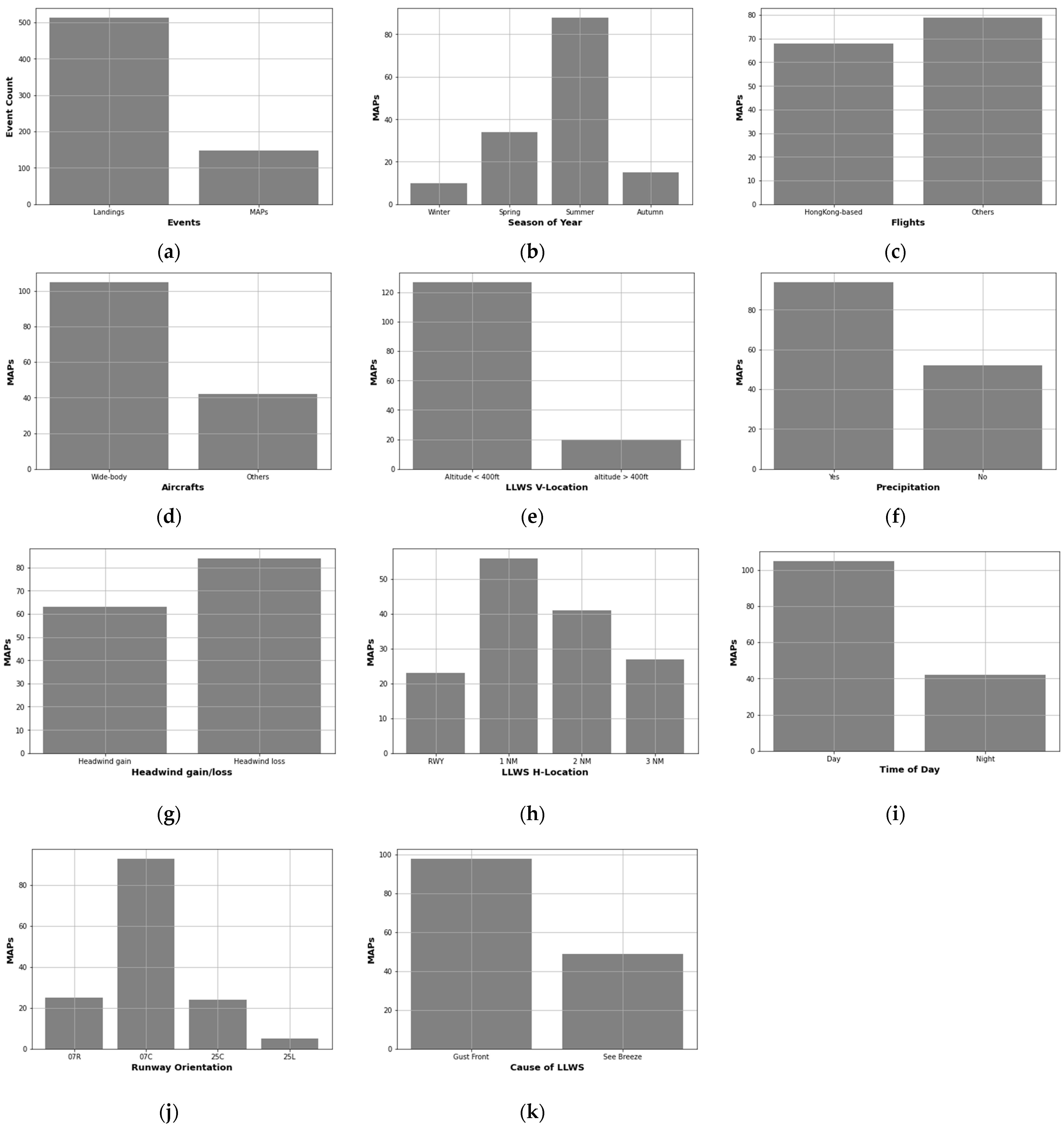
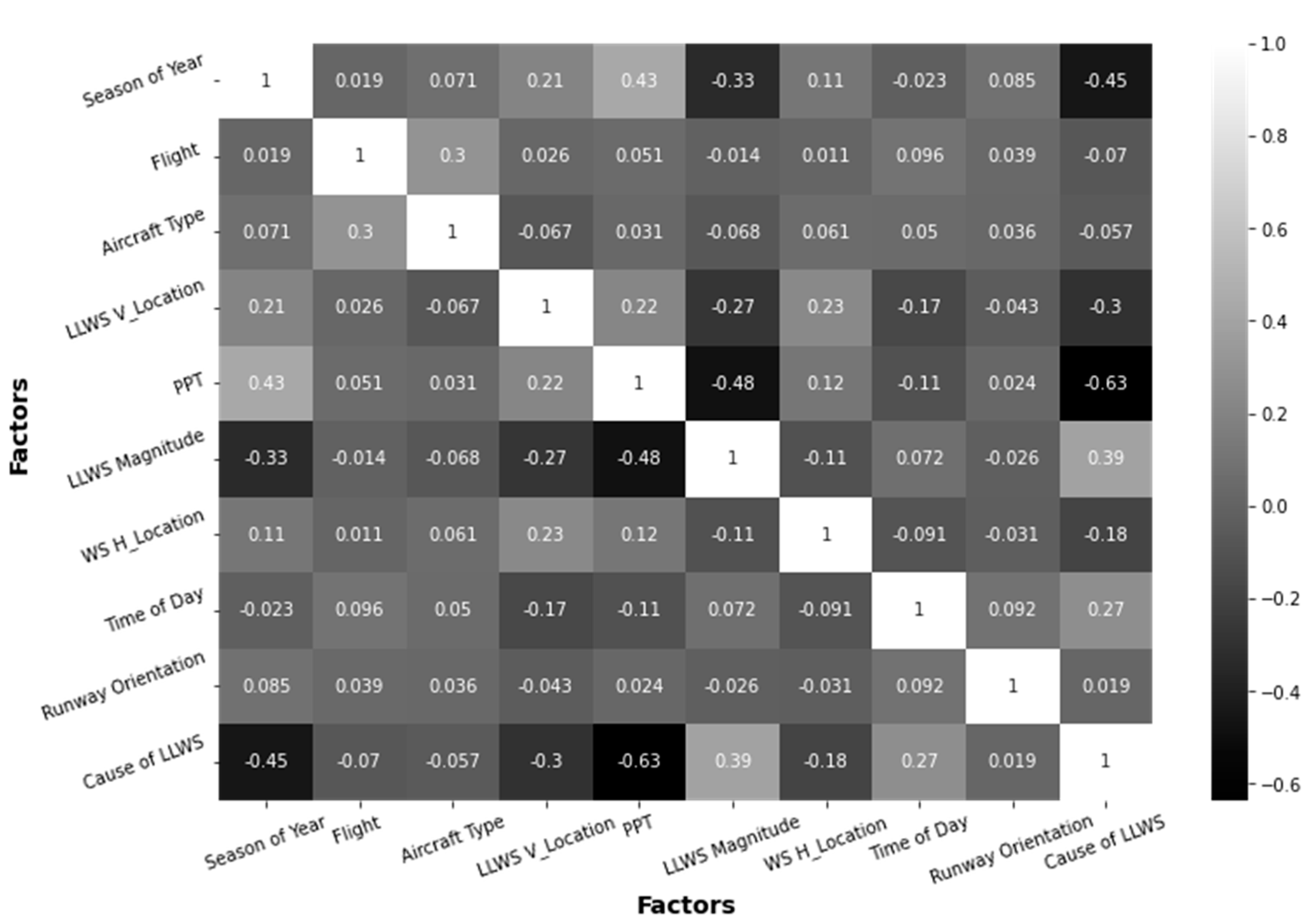
To predict the occurrence of go-around in WS conditions, the DES models with different pools of base estimators were employed by using HKIA-based PIREPs. Figure 6 shows the frequency distributions of the factors from the PIREPs. To assess the potential correlations between the factors of the PIREPs, we performed Pearson correlation analysis. Statistically, Figure 7 illustrates that the absolute value of Pearson’s correlation coefficient is between 1 and −1. Although we have observed a Pearson correlation coefficient value of –0.63 for causes of WS and PPT, the correlation is moderate, and we will not exclude them for subsequent modeling. Both the factors are environmental-specific and their inclusion in the model may have a significant impact. For the analysis, we used the Python sklearn.metrics, imbeans, and sklearn.ensemble, Scikit-learn, and SHAP libraries.

3.1. Data Partitioning

The dataset of 872 go-arounds and approaches under WS conditions that was extracted from HKIA-based PIREPS and used for DES modeling has been split into primarily two sets, which are known as the training validation set and the test set. Seventy percent of the data was used for training validation, while thirty percent of the data was used for actual testing. The training validation set had a total of 468 and 143 records, respectively, for the number of approaches and the go-around events. The testing set included a total of 209 approaches and 53 records of the go-around attempts.

3.2. Grid Search Strategy for Hyperparameter Tuning

Using Stratified 10-Fold Cross-Validation, the training validation set was evaluated. The training validation set was split into 10 equal-sized folds. Utilizing stratified sampling, each fold retained a proportional amount of each label. The Stratified 10-Fold Cross-Validation strategy was chosen because it maintains a proportional representation of each label. The DES model was initially trained with nine folds, and then its F1-Score performance was evaluated with the final fold. This procedure was repeated ten times until all available folds (those that comprised the training set in the initial fold) comprised the validation set. The average F1-Score of each 10 folds was then determined.

Grid Search [43] is one of the most frequently employed hyperparameter tuning techniques for machine learning approaches. Through using the Grid Search technique, the feasible set (search space) of hyperparameters was pre-determined, and the model’s best hyperparameters were chosen based on their performance in cross-validation. For our studies, the model’s hyperparameters were determined by the set of hyperparameters that maximized the overall F1-Score (mean F1-Score across all folds). The F1-Score was chosen as the performance indicator because it combines the recall and precision of diagnostic labels.

Table 6. Optimal hyperparameter values of the models.

Model	Hyperparameter	Space	Optimal Value
RF	Number of trees	[100, 500, 1000, 1500, 2000, 2500, 3000]	2500
	Max depth of tree	[3, 5, 7, 9, 11, 13, 15]	11
BMPL	Number of estimators	[200, 400, 600, 800, 1000]	500
	Batch size	[50, 100, 150, 200, 250, 300]	200
	Epoch size	[50, 100, 150, 200]	110
ERT	Number of trees	[100, 500, 1000, 1500, 2000, 2500, 3000]	2000
	Max depth of tree	[3, 5, 7, 9, 11, 13, 15]	11
SVM	C	[0.1, 1.0, 100]	100
	Gamma	[1.0, 0.1, 0.01, 0.001, 0.0001]	0.01

shows the optimal values of the hyperparameter of the models.

3.3. DES Models’ Performance Assessment and Comparison

As was previously mentioned, the positive and negative classes were referred to as approach and go-around, respectively. The Precision, Recall, and F1-Score performance metrics were extracted from the confusion matrices of each DES algorithm and used to evaluate all models. Homogeneous and heterogeneous pools of classification algorithms were used as the base estimators (

Table 7. Comparison of performance measures of DES algorithms based on the pool of RF.

Approach	Performance Measures
			Predicted		Precision	Recall	F1-Score
			Approach	Go-Around
KNORAE-RF	Actual	Approach	193	16	0.82	0.82	0.82
		Go-around	15	38
DES-P-RF	Actual	Approach	182	27	0.75	0.68	0.71
		Go-around	30	23
META-DES-RF	Actual	Approach	195	14	0.86	0.83	0.84
		Go-around	16	37

,

Table 8. Comparison of performance measures of DES based on the pool of BMLP.

Approach	Performance Measures
	Class		Predicted		Precision	Recall	F1-Score
			Approach	Go-Around
KNORAE-BMLP	Actual	Approach	195	15	0.77	0.75	0.76
		Go-around	22	31
DES-P-BMLP	Actual	Approach	182	27	0.78	0.75	0.77
		Go-around	23	30
META-DES-BMLP	Actual	Approach	195	15	0.73	0.73	0.73
		Go-around	23	30

,

Table 9. Comparison of performance measures of DES based on the pool of ERT.

Approach	Performance Measures
	Class		Predicted		Precision	Recall	F1-Score
			Approach	Go-Around
KNORAE- ERT	Actual	Approach	185	24	0.76	0.73	0.75
		Go-around	24	29
DES-P-ERT	Actual	Approach	184	25	0.75	0.72	0.74
		Go-around	25	28
META-DES-ERT	Actual	Approach	188	21	0.78	0.76	0.77
		Go-around	21	32

and

Table 10. Comparison of performance measures of DES based on the pool of heterogeneous classifiers.

Approach	Performance Measures
	Class		Predicted		Precision	Recall	F1-Score
			Approach	Go-Around
KNORAE-(SVM+KNN+BLR)	Actual	Approach	172	37	0.71	0.72	0.72
		Go-around	21	32
DES-P-(SVM+KNN+BLR)	Actual	Approach	168	41	0.72	0.70	0.71
		Go-around	23	30
META-DES-(SVM+KNN+BLR)	Actual	Approach	188	21	0.78	0.76	0.77
		Go-around	21	32

). META-DES produced a higher performance measure for DES algorithms using RF classifiers as base estimators with Precision (86%), Recall (83%), and F1-Score (84%) (Table 7). KNORAE-RF, the second-best DES model when used with the RF classifier, produced an F1-Score of 82%, a Precision value of 82%, and a Recall value of 82%. Similar to this, DES-P-BMLP produced higher performance measures, with Precision (78%), Recall (75%), and F1-Score (77%), in the case of DES algorithms with BMLP (Table 8). When using the ERT classifier with other DES algorithms, the META-DES performed well (Table 9). It displayed a Precision of 78%, a Recall of 76%, and an F1-Score of 77%. Furthermore, the META-DES with the pool of heterogeneous classifiers (SVM+KNN+BLR) performed well as compared to DES-P and KNORAE (Table 10). It showed a Precision of 78%, a Recall of 76%, and an F1-Score of 77%. Overall, it was found that the META-DES-RF model performed better than the other DES models and could be used in conjunction with SHAP analysis to determine the relative importance of different factors as well as their contributions.

3.4. Sensitivity Analysis

It is vital to develop an evident go-around prediction model because more accurate models might effectively capture the association between go-around and various environmental and situational factors. The ability to comprehend the optimal META-DES-RF model is immensely valuable. The SHAP method was used in this section to interpret the best META-DES-RF results and calculate the combined effect of each individual risk factor.

3.4.1. Global Factors’ Importance and Contribution

We utilized the META-DES-RF model for the factors’ importance and contribution analysis due to its superior go-around prediction compared to other models. There is a compelling case for determining which factors are most crucial and for quantifying their contributions to the final predictions. It is important to note that factor contribution and factor importance are two different concepts. The importance of a factor reveals which variables have the biggest effects on a model’s performance. The factor contributions not only point out important factors but also give a logical justification for the observed result, in our case “go-around” and “approach.”

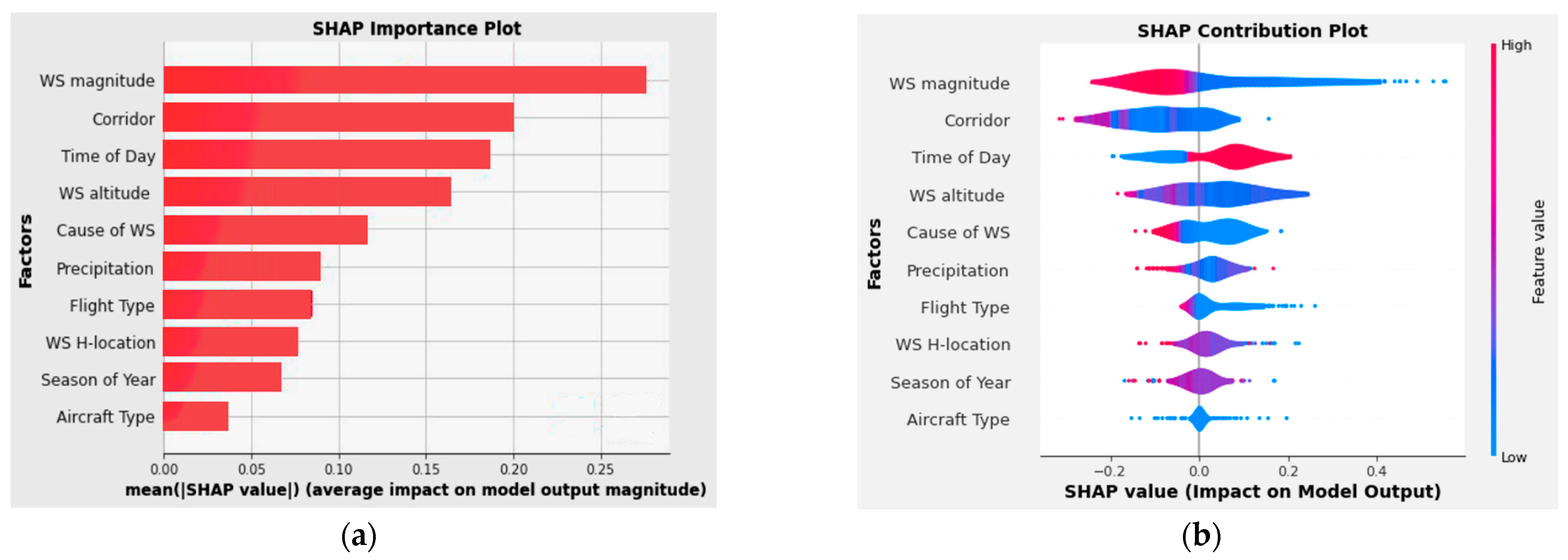
The SHAP global importance scores for the factors used in the META-DES-RF are shown in Figure 8a. The result does not, however, show how much each factor contributed to the likelihood of a go-around happening. It demonstrates that WS magnitude, with a mean SHAP value of +0.257, was the most significant factor that contributed to the occurrence of go-arounds, followed by corridor, with a mean SHAP value of +0.190, time of day (+0.190), and WS altitude (+0.160). Similar to this, a SHAP contribution evaluation was carried out to examine the META-DES-RF model in greater detail using SHAP beeswarm plots (Figure 8b). From the SHAP contribution plots, which combined the Shapely values and expressed the contributions of the various factors to the META-DES-RF model, we were able to derive a quantitative value. On the vertical axis, the input factors are arranged from most influential to least influential in order of increasing influence. The horizontal axis displays the SHAP value, and the color scale, which ranges from blue to red for low significance to high significance, displays the factor’s significance.

The META-DES-RF model’s SHAP beeswarm plot showed that majority of the tailwind led to the commencement of the aircraft go-around. The cause may be that in strong tailwinds, an aircraft’s airspeed—the speed of the aircraft relative to the airflow around it—does not significantly decrease as it approaches the ground, and with a high airspeed, an aircraft may not be able to land at the designated touchdown location. Pilots increase the throttle to go around, try again, or ask for a different runway to ensure safety. The outcome is also in line with earlier research [44]. The second important factor was the corridor’s orientation. Runways 07C and 07R were more likely to initiate go-arounds when there was wind shear. Runways 07C and 07R should not be used for landings during WS events because go-arounds have become a safety concern. The third crucial factor was the time of day. Although we could not pinpoint any prior research on the effect of the time of day on the go-around, our data nonetheless revealed that majority of the go-around happened during the day (07:00 AM to 19:00 PM).

The fourth crucial factor was WS altitude. Figure 8b illustrates how WS events that took place at lower altitudes were held responsible for the high number of go-arounds. This is also consistent with a previous study [45]. The cockpit remains incredibly active during the landing phase, and the captain and co-pilot must make a number of quick decisions to wrap up their landing checklist. However, the best course of action is to abort the landing and perform a go-around when an unexpected WS happens very close to the runway. As a result, majority of go-arounds happened when the aircraft ran into WS close to the ground.

3.4.2. Factor Dependence and Interaction

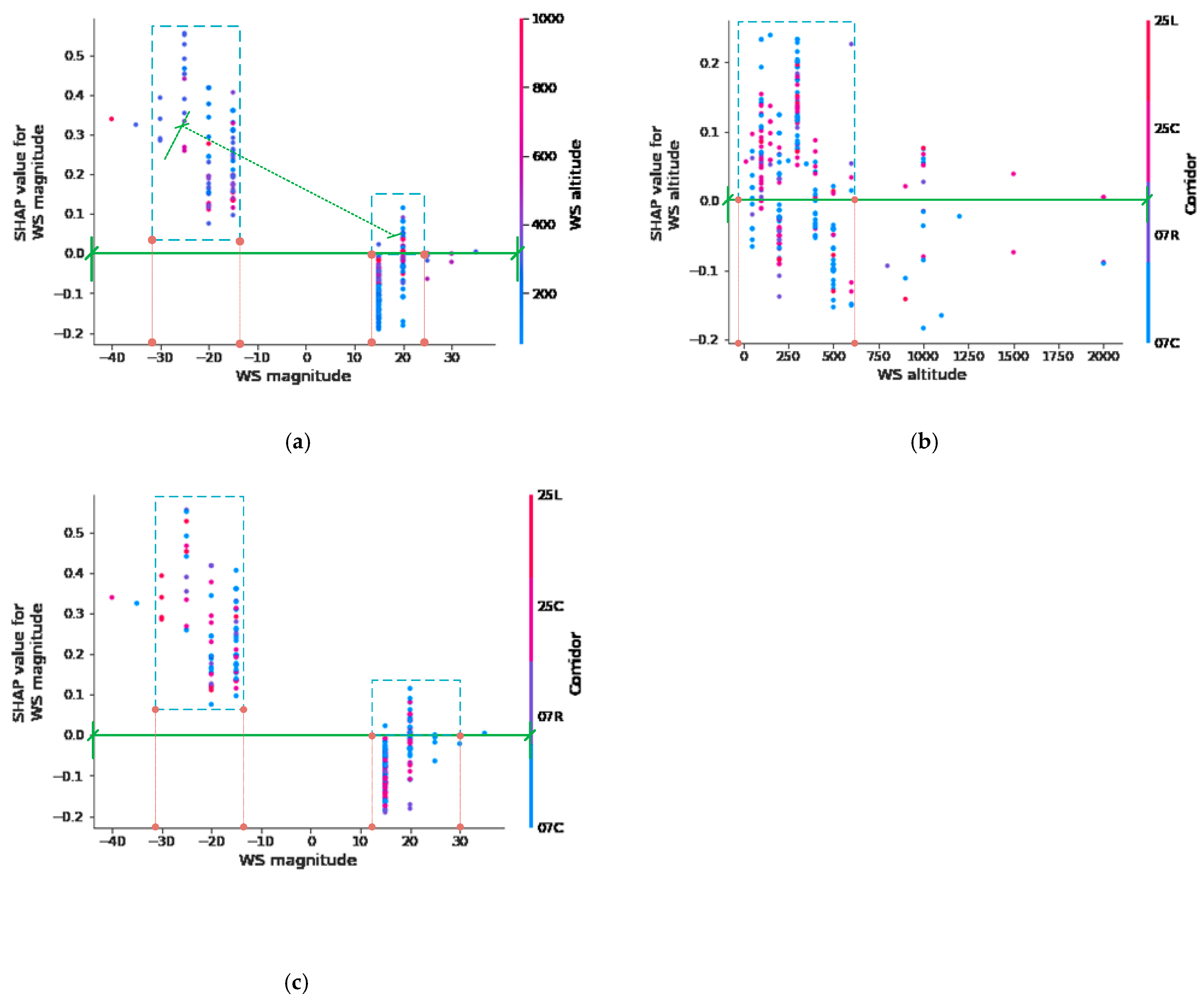
In the factor importance and contribution (beeswarm) plots, there was no evidence of a correlation between the alteration in the factor value and the change in the SHAP value. The interpretation results for the factors are shown in Figure 9, which also adds more relevant information about how the SHAP values varied with the eigenvalues to the contribution plot. To assess the extent to which the critical environment factors used to evaluate the META-DES-RF interacted in terms of their contributions, the SHAP interaction plots were examined.

Figure 9a shows how the models’ predictions were impacted by the WS magnitude and WS altitude. The go-around phenomenon is heavily influenced by the points that are above the SHAP 0.00 green reference line. Thus, it is evident that the points with magnitudes of −14 to −32 knots are above the SHAP 0.00 green reference line. Most of the points have labels in blue and purple, which indicate low altitude between 0 and 600 feet. It shows that strong tailwinds at low altitudes play a greater role in the occurrence of go-arounds. Figure 9b depicts how the WS altitude and Corridor influenced the model predictions. It is apparent that the points with high density that fall between WS altitudes of 0 and 600 feet are located above the SHAP 0.00 green reference line. Majority of the points have blue and purple labels, which denote corridors 07C and 07R. It demonstrates that runways 07C and 07R are highly susceptible to the occurrence of WS at low altitude, thereby increasing the likelihood of a go-around.

Figure 9c illustrates the effect of the WS magnitude and Corridor on model predictions. Clearly, the dense points that fall between WS altitudes of −14 and −32 knots are located above the SHAP 0.00 green reference line. A significant proportion of the points is marked with blue and purple labels, denoting corridors 07C and 07R. It reveals that runways 07C and 07R are particularly prone to the occurrence of WS at −14 to −32 knots (tailwind condition), as well as the low altitude of WS, thereby boosting the likelihood of a go-around.

4. Conclusions and Recommendations

In this study, a Dynamic Ensemble Selection model was used with a pool of homogeneous (Random Forest, Extremely Randomized Tree, and Bagging Multilayer Perceptron) and heterogeneous (Support Vector Machine, K-Nearest Neighbor, and Binary Logistic Regression) classifiers to predict the occurrence of go-arounds using the Hong Kong International Airport-based Pilot Reports from 2018 to 2021. The META-DES-RF model outperformed all the other models in terms of the Precision value, the Recall value, and the F1-Score. As a result, the META-DES framework that has been proposed presents a novel approach to modeling and forecasting aircraft go-around in WS conditions.

The lack of inclusivity and interpretability of machine learning models has been widely criticized. Although these approaches are often more flexible and reliable than traditional statistical models, this hinders their widespread adoption for prediction. Therefore, in this study, the results of META-DES-RF were evaluated, and both key risk factors and their impact on the occurrence of go-around were analyzed using the SHAP strategy to deal with the problem of interpretability introduced by META-DES-RF.

The top four crucial risk factors that enhance the probability of the occurrence of go-around under WS events were WS magnitude, Corridor, time of day, and WS altitude. The SHAP analysis revealed that there was a strong interaction among WS magnitude, WS altitude, and Corridor. It has been observed that runways 07C and 07R of HKIA were more prone to the occurrence of go-around. These go-around events occurred when strong tailwinds of −14 to −32 knots occurred within 600 ft above the runway level.

The novel method used in this research could be applied to a comprehensive investigation of how WS events have affected air traffic operations. It is a helpful tool for experts in air traffic safety and decision-makers in the aviation industry. In this study, SHAP analysis and dynamic ensemble classifiers were only used to predict the aircraft go-around under WS events. Future research initiatives may employ additional DES algorithms with various pools of classification models and risk factors. Doppler LiDAR data could also be combined with PIREPs in future research to evaluate a wide range of other parameters, including the impact of pressure, the direction of the wind, and others.