Prediction of a Pilot’s Invisible Foe: The Severe Low-Level Wind Shear

Abstract

Severe low-level wind shear (S-LLWS) in the vicinity of airport runways (25 knots or more) is a growing concern for the safety of civil aviation. By comprehending the causes of S-LLWS events, aviation safety can be enhanced. S-LLWS is a rare occurrence, but it is hazardous for approaching and departing aircraft. This study introduced the self-paced ensemble (SPE) framework and Shapley additive explanations (SHAP) interpretation system for the classification, prediction, and interpretation of LLWS severity. Doppler LiDAR- and PIREPs-based LLWS data from Hong Kong International Airport were obtained, trained, and evaluated to predict LLWS severity. The SPE framework was also compared to state-of-the-art tree-based models, including light gradient boosting machine, adaptive boosting, and classification and regression tree models. The SPE does not require prior data treatment; however, SMOTE-ENN was utilized to treat highly imbalanced LLWS training data for tree-based models. In terms of prediction performance, the SPE framework outperforms all tree-based models. Using SHAP analysis, the SPE was interpreted. It was determined that “runway 25LD”, “mean hourly temperature”, and “mean wind speed” were the most significant contributors to the occurrence of S-LLWS. The most optimistic projections for the occurrence of S-LLWS events at runway 25LD were during periods of low-to-moderate temperatures and relatively medium-to-high wind speeds. Similarly, the majority of S-LLWS events took place on the runway. Without the need for data augmentation during preprocessing, the SPE framework coupled with the SHAP interpretation system could be utilized effectively for the prediction and interpretation of LLWS severity. This study is an invaluable resource for aviation policymakers and air traffic safety analysts.

1. Introduction

Airline operations are profoundly impacted by weather conditions. Major causes of flight cancellations, delays, and even fatal crashes [1,2,3] can be traced back to this concern. Wind shear refers to an abrupt shift in the wind’s speed or direction in the atmosphere. Particularly during landing and takeoff, aircraft are impacted by low-level wind shear (LLWS), which is present in a lower layer at 1600 feet above ground level (AGL). LLWS is defined by the International Civil Aviation Organization (ICAO) [4] as a 15-knot-or-greater change in wind direction at or below 1600 feet above ground level. It affects the aircraft’s lift, and the resulting course deviation could endanger planes taking off or landing [5,6].

Many LLWS events with a magnitude of 25 knots or higher have been registered at airports around the world. Because S-LLWS may have a stronger impact on aircraft operations, timely warnings are crucial. Hong Kong International Airport is one of the most at-risk airports for LLWS (HKIA). It is located in Lantau Island’s northern region, which is mountainous, with peaks reaching over 900 m and valleys dropping to 300 m. Lowering the adverse effects of S-LLWS on airport safety and productivity is vital. A reliable LLWS severity prediction approach is crucial for achieving the goal of providing precise and effective wind hazard alerts and ensuring the safety of civil aviation. The development of models for predicting the severity of LLWS closer to airport runways, however, remains among the most challenging areas of research in civil aviation today.

Due to the fact that wind shear exhibits characteristics of meso- and micro-scale meteorological phenomena, such as abrupt changes in speed and direction and a small temporal–spatial scale, predicting wind shear is a difficult endeavor. LLWS events occur in both rainy and non-rainy weather and include phenomena such as frontal gusts and microbursts associated with severe convection, dry microbursts, low-level jets, sea breezes, complex terrain effects, etc [7]. To ensure the safety of civil aircraft, various technologies, including anemometers, terminal Doppler weather radar (TDWR), and Doppler light detection and range (DLDR), have been installed at major airports around the world to detect LLWS (LIDAR). Few airports, including those in Japan, Malaysia, the United States, Germany, France, South Korea, Singapore, and Hong Kong, have LLWS alerting technologies due to high instrument and maintenance costs, a lack of relevant research, and unique local environments [8]. The anemometer-based LLWS alert system and the TDWR have been developed since the 1970s. Their effectiveness for detecting and warning of LLWS in rainy conditions has been demonstrated [9]. The complementary TDWR is also capable of detecting LLWS caused by terrain. However, these technologies are incapable of capturing LLWS events in non-rainy weather [10,11] and are unsuitable for detecting LLWS along the glide path.

Doppler LIDAR [8], a relatively new remote sensing technology, offers a promising alternative for detecting LLWS when the weather is clear. Similarly, certain LLWS events are terrain-induced LLWS phenomena caused by the complex terrain surrounding an airport. Doppler LIDAR technology, which does not depend on humid conditions for detecting LLWS and captures LLWS due to complex terrain near airports, has been developed to address these scenarios. Hong Kong International Airport [12], Nice Côte d’Azur Airport in France [13], Tokyo Haneda International Airport in Japan [14] and Beijing Capital International Airport in China [15] are equipped with the Doppler LIDAR system. It has been added to the TDWR as an augmentation in order to detect and warn of LLWS, even in clear skies. However, the development of a model to predict the severity of LLWS based on Doppler LIDAR observations remains a challenging task that must be addressed. Similarly, all of these LLWS alerting technologies (based on remote sensing and/or on-site measurements) have been proven effective and operational. These technologies send notifications or alerts when LLWS events are detected or observed. However, these hardware-based technologies are incapable of predicting the occurrence of LLWS events and assessing the risk factors that contribute to their occurrence [16].

In the past, numerous numerical modeling techniques, including large-eddy simulations (LES) [17], computational fluid dynamics (CFD) [18] and numerical weather prediction (NWP) [12] have been employed to attempt to predict or simulate wind shear conditions. In general, these studies focused on single or isolated occurrences of reported wind shear events and were conducted on a case-by-case basis. There are insufficient systematic, long-term evaluations of the ability of numerical models to predict the occurrence of LLWS events. These days, machine learning algorithms have gained significant ground. It has become one of the most widely used and beneficial tools in transportation research such as road safety, transportation planning, and pavement analysis [19,20,21,22]. However, there is a significant gap in the application of machine learning algorithm in the aviation safety domain, particularity in the prediction and classification of LLWS severity. In this research, efficiently predicting S-LLWS is of interest to us. However, in the data from LiDAR and pilot reports (PIREPs), the S-LLWS class is typically much smaller than the non-severe low-level wind shear (NS-LLWS) class. This creates a data imbalance issue and requires data balancing prior to training and evaluation. Therefore, in contrast to hardware-based technologies and numerical simulation modeling, which efficiently predict LLWS severity while simultaneously dealing with the class imbalance issue, we propose the self-paced ensemble (SPE) framework [23]. This is an ensemble imbalance learning model for dealing with highly imbalanced data. It aims to produce a robust ensemble by the self-paced harmonizing of data hardness via the undersampling method that has been developed. This framework, despite being computationally efficient, has resulted in robust performances in the presence of extremely skewed distributions.

Although machine learning models are efficient in prediction, they do not explicitly demonstrate the relations between input and output factors due to their black-box nature. The interpretation of the model is equally important for appropriately assessing the model’s performance. Previously, the machine learning model’s results were interpreted using the variable importance analysis methods such as permutation-based importance scores. The variable importance analysis, however, can only provide a ranking of the variables’ importance and is unable to explain how each variable individually influences the prediction of the model. Shapley additive explanations (SHAP) analysis, based on the concept of game theory [24], has been utilized in recent studies to quantify each factor’s effect on the outcome [25,26]. In this research, we have also employed SHAP, analysis in conjunction with SPE framework, for the assessment of the relative importance of various factors as well as their contributions.

The rest of this paper is organized as follows: The following sections constitute the research methodology, which provides the data description, the details of the proposed SPE framework, a Bayesian optimization strategy for hyperparameter tuning, and the description of the SHAP interpretation system. These are then followed by Section 3, discussing the SPE framework and comparison with other machine learning models, as well as SHAP analysis. Finally, Section 4 summarizes the conclusions and makes additional research recommendations.

2. Materials and Methods

Initially, the LLWS data consisted of LiDAR data and pilot flight reports (PIREPs) obtained from the Hong Kong Observatory (HKO) at HKIA. The details of data extraction from LiDAR and PIREPs are provided in the subsequent section. The extracted data were merged together and preprocessed to separate training–validation and testing datasets into 70% and 30%, respectively. The training dataset was used to develop an SPE framework and tree-based machine learning models, including light gradient boosting machine (LGBM), adaptive boosting (AdaBoost), and classification and regression tree (CART), and the testing dataset was used to evaluate the performance of the developed model. The SPE framework is an ensemble imbalance learning system, which does not require data balancing during the preprocessing phase. In contrast, data balancing was required for the tree-based machine learning models prior to training and validation, which were used to compare the results with the SPE framework. For data balancing, a hybrid synthetic minority oversampling technique—edited nearest neighbor (SMOTE-ENN) treatment was applied to the LLWS training dataset. A portion of the training–validation data were also used to tune model hyperparameters. A Bayesian optimization approach was utilized for the hyperparameter tuning. Afterwards, the SHAP interpretation system was used to evaluate the significance and contribution of various risk factors that generate S-LLWS in the vicinity of airport runways. In addition, factor interaction analysis by SHAP was also conducted. Figure 1 depicts the entire operational paradigm described in this study.

2.1. Study Location

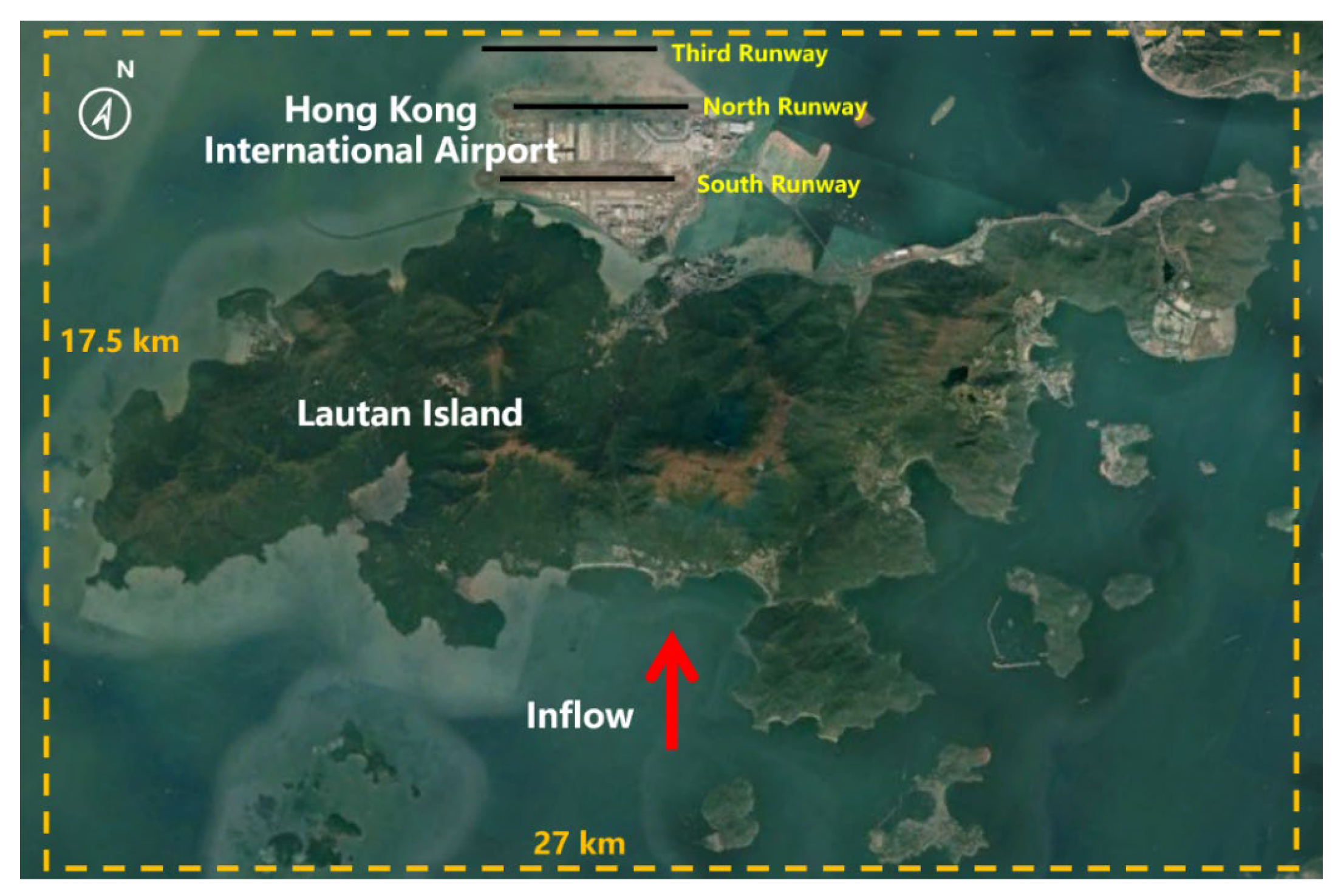
The Hong Kong International Airport (HKIA) is situated on an artificial island called Lantau, which is surrounded on three sides by water. To the south, there are mountains that rise to more than 900 m above sea level. The complex land–sea contrast and intricate orography of HKIA have been the subject of numerous observational and modeling studies, all of which have identified that they are favorable conditions for the occurrence of LLWS [27,28]. As seen in Figure 2, the mountainous area to the south of HKIA amplifies LLWS, disrupting airflow and causing mountain waves, gap effluents, and other disruptions along the HKIA flight paths. The north runway and the south runway are the two runways at HKIA. The directions they orient are 070° and 250°. Eight different arrangements are possible because each runway can be used for takeoffs and landings in either direction. For instance, runway ‘07LA’ stands for a landing (‘A’ stands for arrival) using the left runway (hence ‘L’) and a heading angle of 070°. This depicts a plane landing on HKIA’s north runway from the west. The same goes for an aircraft taking off from the south runway and heading west—runway 25LD.

2.2. Instrument and Data

In this section, the Doppler LiDAR of HKIA and the pilot flight reports (PIREPs) of HKIA inbound and outbound flights, are thoroughly discussed.

2.2.1. Doppler LiDAR at HKIA

In this study, LLWS data gathered from the 2 × long-range Doppler LiDAR at HKIA were analysed. LiDAR operates at an infrared wavelength of approximately 1.5 microns; 100 m is the radial resolution or physical range gate. Maximum radial velocity is roughly 40 m per second. Typically, under ideal weather conditions and in the absence of obstructions such as low clouds, an observation range of 10 or 15 kilometres is achievable. In addition to the standard fixed-elevation scans (plan-position indicator), each LiDAR is configured to conduct “glide-path” scans along take-off and landing flight paths. Coordinating the elevation and azimuth movements of the laser scanner head accomplishes this. Typically, the four possible configurations of the north runway (07LA, 25RA, 07LD, and 25RD) are covered by the north LiDAR, including arrivals (A) and departures (D) directions, and the four possible configurations of the south runway (07RA, 25LA, 07RD and 25LD) are covered by the south LiDAR, including arrivals (A) and departures (D) directions towards the west and the east. The headwind component along each runway configuration (labelled “corridor”) can be derived from the “glide-path” scans’ radial velocity data. Typically, the scan revisit time for each corridor is roughly one minute, indicating that the temporal resolution or update frequency of the headwind profiles is also roughly one minute.

The LiDAR at HKIA usually operates by a “GLYGA LLWS alerting algorithm” [7]. For each runway corridor, GLYGA receives as input the profile of headwind components gridded with a 100 m interval. The headwind profiles typically extend up to 4–5 NM from the respective runway endpoint, based on scanning range and prevalent atmospheric conditions at the time. Then, a ramp identification procedure is used to identify sudden, consistent changes in the headwind. This is based on the “Peak Spotter” algorithm [29]. First, a profile of velocity increment is quantified by adjusting adjacent data points from the profile of quality-controlled headwind. Next, LLWS “ramps” are identified by sequentially recognizing the velocity increment (i.e., headwind change) within length windows of 400, 800, 1600, and 6400 m. The collection of such “ramps”, identified within a single headwind profile, is then ranked using a severity factor [30] that scales with the headwind increment and the inverse cube root of the ramp length. The ramp with the highest severity factor is then used to release an automatic alert when intensity exceeds a predetermined threshold (15 knots) at HKIA.

Mathematically, the quality-controlled headwind profile can be represented as $\upsilon \left(x_k\right)$, where $\upsilon$ is the headwind component at the $x_k$ position, which is the $k$th data point or range gate along the corresponding glide path. The velocity increment at location $x_k$ can be expressed as $\mathrm{\Delta }\upsilon \left(x_k,\lambda \right)=\upsilon \left(x_k\right)-\upsilon \left(x_k+\lambda \right)$ for a given length window (or ramp length), $\lambda$. (For a detailed explanation of the ramp identification process at HKIA, please see [7].) The resultant identified ramps, which correspond to a collection of data pairs $\left(\mathrm{\Delta }\upsilon ,\lambda \right)$, are then ranked by the severity factor ${\mathcal{F}}_s$, which is computed using Equation (1).

$${\mathcal{F}}_s={\left(\frac{\mathrm{\Delta }\upsilon }{\lambda }\right)}^3/{\mathrm{\Phi }}_{app}$$

(1)

where ${\mathrm{\Phi }}_{app}$ denotes the aircrafts’ approach speed, which is taken as constant. The ${\mathcal{F}}_s$ depends primarily on $\mathrm{\Delta }\upsilon /\lambda$.

2.2.2. HKIA-Based PIREPs

Pilot flight reports (PIREP) of LLWS are an established source for confirming LLWS alerts at HKIA. A PIREP is an abbreviation for pilot reports used in the aviation sector. It is a report that pilots who encounter hazardous weather conditions send to air traffic controllers. Typical PIREPs cover the flight’s en route phase and include information on turbulence and aircraft icing. However, the HKIA wind shear PIREPs contain information regarding the timing, location (to the nearest nautical mile), altitude (to the nearest 50 or 100 feet), and velocity (to the nearest 5 knots) of an LLWS event. Pilots can report LLWS events to the air traffic controller at HKIA in two standard ways: by submitting a report form after landing or departure, or by using an on-board radio communication.

2.3. Data Processing

As discussed early, the occurrence of S-LLWS is a substantial risk to inbound and outbound flight safety. Therefore, in order to predict the S-LLWS events, in this study, the occurrence of LLWS severity is defined by the threshold, as shown in Equation (2).

$$\mathrm{LLWS} \mathrm{Severity}=\left\{\begin{array}{cc}1: \mathrm{S}-\mathrm{LLWS},& \mathrm{LLWS} \ge 25 \mathrm{knots}\\ 0: \mathrm{NS}-\mathrm{LLWS},& \mathrm{LLWS} 15 - 24 \mathrm{knots}\end{array}\right.$$

(2)

The original wind shear dataset contains nominal and continuous factors as well as a single target factor, LLWS severity. S-LLWS events represent all LLWS with a magnitude of equal to or greater than 25 knots and are coded as 1, whereas NS-LLWS events have a magnitude between 15 to 24 knots and are coded as 0. S-LLWS events are far less in number than NS-LLWS, but they are an important class for aviation safety. Any $i$th event in the original dataset can be represented as $\left(X_i,y_i\right)=\left(C_i,N_i,y_i\right)$, where $C_i$ is the continuous factor, $N_i$ is the nominal factor and $y_i$ is the target factor. As indicated in

Table 1. One-hot encoding of categorical factors for the modeling.

Factor	Codes and Description
LLWS Severity	1: If LLWS magnitude is equal to greater than 25 knots, 0: ‘Otherwise’
Runways
07LA	1: If a wind shear event is reported at Runway 07LA, 0: ‘Otherwise’
07LD	1: If a wind shear event is reported at Runway 07LD, 0: ‘Otherwise’
07RA	1: If a wind shear event is reported at Runway 07RA, 0: ‘Otherwise’
25RD	1: If a wind shear event is reported at Runway 25RD, 0: ‘Otherwise’
25LA	1: If a wind shear event is reported at Runway 25LA, 0: ‘Otherwise’
25LD	1: If a wind shear event is reported at Runway 25LD, 0: ‘Otherwise’
25RA	1: If a wind shear event is reported at Runway 25RA, 0: ‘Otherwise’
25RD	1: If a wind shear event is reported at Runway 25RD, 0: ‘Otherwise’
Location of Occurrence
1MD	1: If a wind shear event is reported at 1MD from Runway, 0: ‘Otherwise’
1MF	1: If a wind shear event is reported at 1MF from Runway, 0: ‘Otherwise’
2MD	1: If a wind shear event is reported at 2MD from Runway, 0: ‘Otherwise’
2MF	1: If a wind shear event is reported at 2MF from Runway, 0: ‘Otherwise’
3MF	1: If a wind shear event is reported at 3MF from Runway, 0: ‘Otherwise’
RWY	1: If a wind shear event is reported at Runway, 0: ‘Otherwise’
Time of the Day
Day Time	1: If a wind shear event is reported during daytime, 0: ‘Otherwise’
Night Time	1: If a wind shear event is reported during nighttime, 0: ‘Otherwise’

, the nominal factors $N$ of the dataset are one-hot encoded. Each nominal value in the dataset is translated into a new column, and the column is assigned a 0 or 1 value. The number of columns is equal to the number of nominal values. For example, an eight-column matrix is created from a nominal factor “Runway” with eight different values (07LA, 07LD, 07RA, 07RD, 25LA, 25LD, 25RA, 25RD). The continuous features of the datasets, on the other hand, are normalized as stated in Equation (3).

$${\mathrm{C}}_{i,j}^{norm}=\frac{{\mathrm{C}}_{i,j}^{orig}-{ \min \mathrm{C}}_j}{\max {\mathrm{C}}_j-{ \min \mathrm{C}}_j}$$

(3)

where ${\mathrm{C}}_{i,j}^{norm}$ represents the $j$th normalized continuous factors of the $i$th instance of the data. ${\mathrm{C}}_{i,j}^{orig}$ represents the original $j$th continuous factors in the $i$th instance of the data. The ${\min \mathrm{C}}_j$ and $\max {\mathrm{C}}_j$ represent the minimum and maximum of the $j$th continuous factor in the original wind shear dataset, respectively.

Finally, there are 18 factors in the standardized wind shear dataset. The standardized original wind shear dataset consists of the normalized continuous factors (2 factors including hourly temperature and wind speed) as well as one-hot encoded nominal factors (16 factors).

2.4. Self-Paced Ensemble Framework

We propose a newly developed SPE framework, which is an ensemble-based imbalance learning framework, to develop a classification and prediction model for S-LLWS using untreated data from LIDAR and PIREPs. Before employing the SPE framework, we present the concepts of hardness harmonization and a self-paced factor.

2.4.1. Hardness Harmonization

All majority class samples are divided into $k$ bins, where $k$ a hyperparameter, based on their hardness values. Each $k$th bin represents a particular level of hardness. Then, majority class instances are undersampled to create a balanced dataset by maintaining the same total hardness contribution in each bin. Such a method is referred to as “harmonize” in the literature of gradient-based optimization. A similar strategy has been adopted here to harmonize the hardness in the initial iteration. However, hardness harmonization is not utilized in every iteration. The primary reason for this is that the number of trivial samples increases during the training process, as the ensemble classifier gradually conforms to the training set. Consequently, merely harmonizing the hardness contribution leaves a large number of trivial samples. Later iterations of the learning procedure are significantly slowed down by these less informative examples. In lieu of this, “self-paced factors” have been introduced to perform the self-paced harmonization of undersampling.

2.4.2. Self-Paced Factor

In particular, after harmonizing the hardness contribution of each bin, the sample probability of bins with a large population is gradually decreased. The rate of decrease is determined by a self-paced factor $\left(\mathsf{\sigma }\right)$. When $\mathsf{\sigma }$ is large, more focus is on the harder samples as opposed to the simple hardness contribution harmonization. In the initial few iterations, the framework focuses primarily on informative borderline samples, and so outliers and noise have little impact on the model’s ability to generalize. In later iterations where $\mathsf{\sigma }$ is very large, the framework retains a reasonable proportion of trivial (high confidence) samples as the “skeleton”, thereby preventing over-fitting. The detail of SPE framework is shown in Algorithm 1. It is pertinent to mention that the hardness value in each iteration (line 5–6) is updated in order to select those data samples that were most beneficial for the current ensemble. The tangent function (line 8) has been used to control the growth of the self-paced factor. Thus, the self-paced factor is equal to zero in the first iteration and to infinity in the last iteration.

Algorithm 1: Self-Paced Ensemble (SPE) Framework.
1	Input: Hardness function $\left(\hslash \right)$, training dataset $D={\left\{\left(x_k{,y}_k\right)\right\}}_1^n$, number of bins $\left(k\right)$, base classifier $\left(\mathsf{\zeta }\right)$ and number of base classifiers $\left(\partial \right)$
2	Initialize:${\rm P}\Leftarrow$ minority class in training dataset $D$$, N\Leftarrow$ majority class in training dataset $D$,
3	Train classifier ${\mathsf{\zeta }}_0$ $\mathrm{by} \mathrm{using} \mathrm{random} \mathrm{undersampling} \mathrm{of} \mathrm{subsets} \mathrm{of} \mathrm{majority} \mathrm{class} N_0{}^{\prime }$ and ${\rm P}$ such that where $\left|N_0{}^{\prime }\right|=\left|{\rm P}\right|$
4	for $\mathrm{i}=1 \mathit{to} n$do
5		Ensemble $F_i\left(x\right)=\frac{1}{i}{\displaystyle \sum _{j=0}^{i-1}{\mathsf{\zeta }}_j}\left(x\right)$
6		Separate majority class dataset into k bins with respect to $\hslash \left({x,y,F}_i\right)$$:\left(b_1{,b}_2,\dots {,b}_{\xi }\right)$
7		In the $l$th bin, the average hardness contribution can be computed as $h_l={\displaystyle {\sum }_{s\in b_l}h}\left(x_s{,y}_s{,F}_i\right)/\left|b_l\right|, \forall l=1,2,\dots ,k$
8		The self-paced factor is updated as $\mathsf{\sigma }=\mathit{tan}\left(\frac{i\mathrm{\Pi }}{2\partial }\right)$
9		$\mathrm{The} l$th bin, non-normalized sampling weight: $p_l=\frac{1}{h_l+\mathsf{\sigma }},\forall l=1,2,\dots ,k$
10		Undersampling from the $l$th $\mathrm{bin} \mathrm{with} \frac{p_l}{{\displaystyle {\sum }_m{p}_l}}\left|{\rm P}\right|$ samples
11		Using newly undersampled data subset, train ${\mathsf{\zeta }}_i$
12	End
13	Return Final robust ensemble $F\left(x\right)=\frac{1}{\partial }{\displaystyle \sum _{m=1}^{\partial }{\mathsf{\zeta }}_m}\left(x\right)$

2.5. Bayesian Optimization for Hyperparameter Tuning

In this study, a Bayesian optimization strategy [31] is employed alongside SPE models and a tree-based machine learning model to determine the optimal hyperparameters. The Bayesian optimization built a probability model for determining the value, which automatically reduces the objective function based on the objective’s prior estimation result. Figure 3 is a flowchart of a hybrid Bayesian optimization machine learning approach. Additionally, provided below is the detailed procedure.

2.5.1. Initialization

This step involves randomly initializing the appropriate hyperparameter settings (Equation (4)), which can be used to train both the SPE model and machine learning models based on k-fold cross validation. The loss function $\left(L_f\right)$ is additionally initialized.

$$H=\left(\begin{array}{cccc}{h}_{1,1}& h_{1,2}& ..& h_{1,l}\\ h_{2,1}& h_{2,2}& ..& h_{2,l}\\ h_{3,1}& h_{3,2}& ..& h_{3,l}\\ :& :& & :\\ :& :& & :\\ h_{m,1}& h_{m,2}& ..& h_{m,l}\end{array}\right)$$

(4)

2.5.2. Fitness Function

From the initialized values, the solution’s random number is generated. Based on the following Equation (5), the fitness function can be used to minimize the objective function.

$$\mathrm{fitness} \mathrm{function}\left(\frac{L}{H}\right)=\left\{\begin{array}{c}D\left(H\right)\\ G\left(H\right)\end{array}\right.\begin{array}{c}L < L^{*}\\ L\ge L^{*}\end{array}$$

(5)

where $L$ denotes the loss value, $D\left(H\right)$ denotes the density estimation, which is based on the loss value during the observations, $G\left(H\right)$ is produced by the leftover observations value of loss, and $L^{*}$ represents the particular quantiles.

2.5.3. Sequential Model-Based Optimization

For fine-tuning the hyperparameters of SPE and tree-based models, sequential model-based optimization is one of the succinct forms of Bayesian optimization. Sequential model-based optimization operates by finding the optimal hyperparameter setting, $H^{*}$, by building the Gaussian process, ${\mathrm{\Theta }}_z$, with sampled points which can be obtained by the following Equation (6).

$$H^{*}=\arg \min {\mathrm{\Theta }}_{z-1}\left(H\right)$$

(6)

Equation (7) can be used to calculate the loss value under ideal hyperparameter settings.

$$L=L_f\left(H^{*}\right)$$

(7)

The corresponding $L$ and the $H^{*}$ settings are stored in the corresponding trails, which can be represented as $\mathrm{\Omega }$. These corresponding trails $\left(\mathrm{\Omega }\right)$ are used for parameter settings and evaluations purposes. The $\mathrm{\Omega }$ update can be determined with the help of following Equation (8).

$$\mathrm{\Omega }=\mathrm{\Omega }\cup \left(H^{*},L\right)$$

(8)

Finally, build the Gaussian process model, ${\mathrm{\Theta }}_z$, based on updated $\mathrm{\Omega }$.

2.5.4. Acquisition Function

The next iteration of the search process is computed using the acquisition function of Bayesian optimization. The maximization of G-Mean, which is the expected improvement in this study, is chosen as an acceptable performance criterion for the SPE model and tree-based machine learning models. Equation (9) can be used to achieve the improvement.

$$D\left(H\right)=\max \left[\left\{L_{\min }-L\left(H\right)\right\},0\right]$$

(9)

2.5.5. Termination

When the termination criteria are satisfied in this step, the best hyperparameters for the SPE model and tree-based machine learning models are obtained.

2.6. Evaluation of Models

In case of binary classification problem, one class is the majority (the negative) and its sample size is represented by $n_1$; the other class is the minority (the negative) and its sample size is represented by $n_2$. Let $n$ represent the total size of training dataset, ${n=n}_1+n_2$. A binary classifier predicts whether each instance is positive or negative. Therefore, it generates outcomes of four types: true positive $\left(t_p\right)$, false positive $\left(f_p\right)$, true negative $\left(t_n\right)$, and false negative $\left(f_n\right)$ (see confusion matrix Figure 4). The confusion matrix provides an in-depth examination of the model’s performance when predictions are made for each class. The precision and recall are two exceptionally vital model evaluation metrics. The precision is obtained as the ratio of total number of true positives to the total number of true positives and false positives, whereas recall is the ratio of total number of true positives to the total number of true positives and false negatives. Both precision and recall can be computed from the confusion matrix, as shown by Equations (10) and (11), respectively.

However, in ensemble imbalance learning, the imbalanced datasets pose a large challenge to the use of proper metrics for the evaluation of the accuracy in the classification outcomes [32]. The geometric mean (G-Mean), and Matthews’ correlation coefficient (MCC) have been used in various studies instead of classification accuracy or F1-score. MCC values should range between −1 and 1. Values closer to +1 represent improved performance. Both MCC and G-Mean have been generally regarded as a balanced measure which can be used even if the classes are of very different sizes. The expressions for the computation of MCC and G-Mean from confusion matrix are given by Equations (12) and (13).

$$\mathit{Recall}=\frac{t_p}{t_p{+f}_n}$$

(10)

$$\mathit{Precision}=\frac{t_p}{t_p{+f}_p}$$

(11)

$$G-\mathit{Mean}=\sqrt{\left(\frac{t_p}{t_p{+f}_n}\right)\left(\frac{t_n}{f_p{+t}_n}\right)}$$

(12)

$$\mathit{MCC}=\frac{t_p{\times t}_n{- f}_p{\times f}_n}{\sqrt{\left(t_p{+f}_p\right)\left(t_p+f\right)\left(t_n{+f}_p\right)\left(t_n{+f}_n\right)}}$$

(13)

2.7. Interpretation of Model by Shapley Additive Explanations (SHAP)

The SHAP analysis relies on a game-theoretical approach to explain the outputs of the ensemble machine learning classifiers. Since machine learning models are “black boxes”, the core ideas behind the SHAP analysis involve interpreting these models from both a global and local perspective. The SHAP values, which correspond to the value assigned to each factor in the computation of a machine learning prediction, are estimated. The contribution of each factor is determined and displayed as a Shapley value using Equation (14).

$${\phi }_i={\displaystyle \mathsf{\sum }_{\mathsf{\Upsilon }\mathsf{\subseteq }\mathsf{\Pi }\left\{\mathit{i}\right\}}\frac{\mathsf{\Upsilon }!\left(n - \left|\mathsf{\Upsilon }\right| - 1\right)!}{n!}}\left[\mathsf{{\rm E}}\left(\mathsf{\Upsilon }\cup \left\{i\right\}\right) - \mathsf{{\rm E}}\left(\mathsf{\Upsilon }\right)\right]$$

(14)

where ${\phi }_i$ illustrates the $i$th factor contribution, $\mathrm{\Pi }$ the set of all factors, $\mathsf{\Upsilon }$ is the subset of decision factor, $\mathrm{{\rm E}}\left({\mathsf{\Upsilon }}_i\right)$ and $\mathrm{{\rm E}}\left(\mathsf{\Upsilon }\right)$ illustrate the best model results with and without $i$th factors, respectively. SHAP analysis yields the outputs of machine learning models through an additive factors imputation strategy, wherein the output model is defined as a linear sum of the input factors (Equation (15)).

$$g\left({\mathrm{\Psi }}^{\prime }\right){=\mu }_0+{\displaystyle \mathrm{\sum }_{i=1}^{\mathrm{\Lambda }}{\mu }_i}{\mathrm{\Psi }}^{\prime } {\mathrm{\Psi }}^{\prime }\in {\left\{0,1\right\}}^{\mathrm{\Lambda }}$$

(15)

It is equal to 1 in cases when a factor is observed, otherwise it is 0. It illustrates that the amount of all input factors, ${\mu }_0$, represents an outcome without factors (i.e., base value), whereas ${\mu }_i$ shows the Shapley value of factor $i$th.

3. Results and Discussion

In order to predict the severity of LLWS, this study used an effective and cutting-edge SPE framework along with tree-based machine learning models. Python 3.6.6, a free and open-source programming language, was used in this context. For model training, hyperparameter tuning, performance evaluation, and interpretation, we used the Scikit-learn, sklearn.metrics, HyperOpt, and Shap libraries, as well as Python’s sklearn.metrics, imbeans, and sklearn.ensemble. 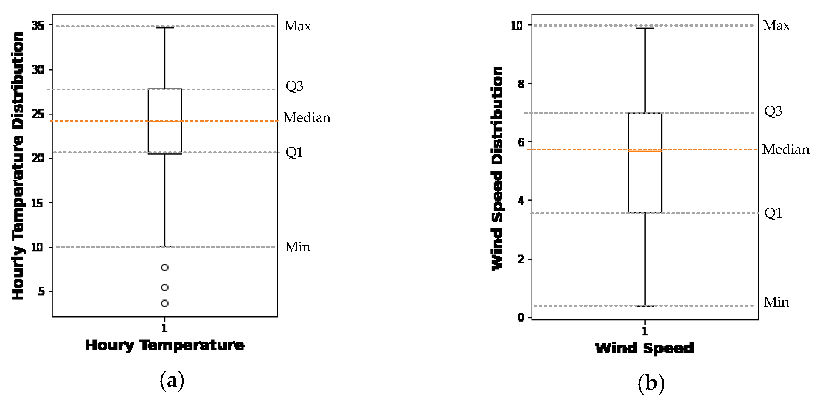Figure 5 shows how LLWS events are distributed in relation to runway orientation, location of occurrence, and time of day. The box plot of the hourly temperature and wind speed is shown in Figure 6. On the training set for tree-based models, the SMOTE-ENN treatment strategy was used. The training–validation dataset contained 257 instances of S-LLWS and 6908 instances of NS-LLWS prior to treatment. The NS-LLWS instances changed into 6518 and 3069 S-LLWS instances, respectively, after the SMOTE-ENN treatment. The performance evaluation was conducted using a testing dataset, and comparisons were made. The best model is then utilized for SHAP analysis.

3.1. Hyperparameter Tuning Using Bayesian Optimization

We used a Bayesian optimization technique that maximized the G-Mean metric to identify the optimal hyperparameters. It is important to note that the SPE framework did not require any prior data treatment, and so imbalanced data were used as input. For tee-based models, both untreated and SMOTE-ENN-treated data were used in the hyperparameter tuning process.

Table 2. Machine learning models hyperparameter tuning.

Treatment	Strategy	Hyperparameters	Range	Optimal Values
No treatment	SPE	n_estimators	[500, 3000]	833
		max_depth	[0, 10]	7
		learning_rate	[0.001, 0.1]	0.077
	LGBM	n_estimators	[500, 3000]	2099
		learning_rate	[0.001, 0.1]	0.043
		max_depth	[0, 10]	5
		lambda_l1	[0.001, 5]	0.39
		lambda_l2	[0.001, 5]	0.22
	AdaBoost	n_estimators	[500–3000]	1873
		Learning_rate	[0.01, 1]	0.056
	CART	min_samples_leaf	[0.05, 0.1]	0.04
		max_depth	[0, 10]	8
SMOTE-ENN	LGBM	learning_rate	[0.001, 0.1]	0.079
		n_estimators	[500, 3000]	2371
		max_depth	[0, 10]	4
		lambda_l1	[0.001, 0.1]	0.57
		lambda_l2	[0.001, 0.1]	0.41
	AdaBoost	n_estimators	[500, 3000]	3110
		learning_rate	[0.001, 0.1]	0.093
	CART	min_samples_leaf	[0.05, 0.1]	0.03
		max_depth	[0, 10]	8

shows the hyperparameters along with their ranges and optimal values.

3.2. Models Performance Assessment and Comparison

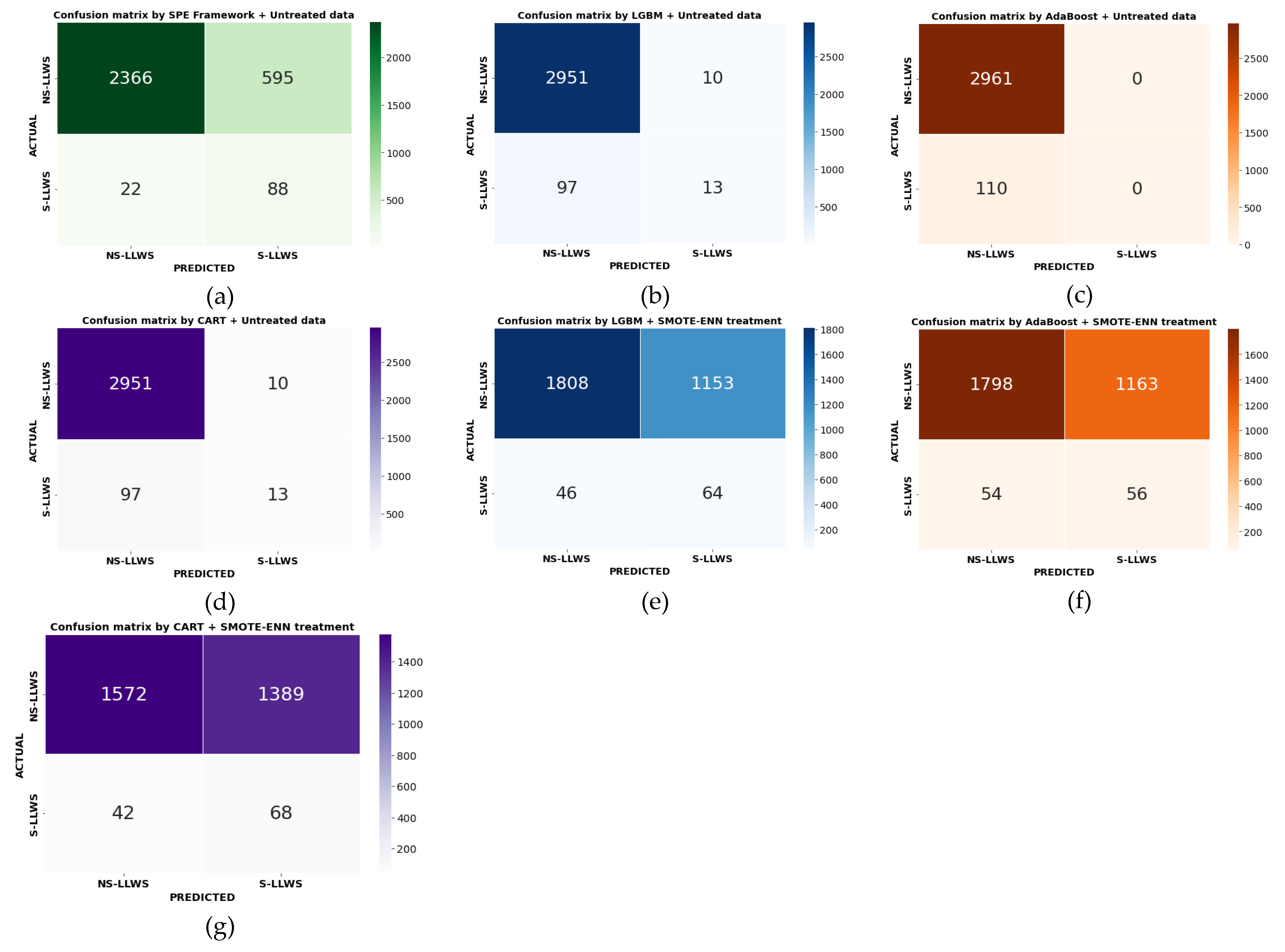
The terms S-LLWS and NS-LLWS events were used in this study to designate positive and negative classes of LLWS, respectively. Different performance measures that were derived from the confusion matrix were used to evaluate each model (Figure 7). The recall value and precision values in

Table 3. Performance measure of machine learning models.

Treatment	Model	Class	Precision	Recall	G-Mean	MCC
No treatment	SPE	NS-LLWS	0.99	0.80	0.82	0.27
		S-LLWS	0.13	0.80
		Average	0.56	0.80
	LGBM	NS-LLWS	0.97	1.00	0.55	0.24
		S-LLWS	0.57	0.12
		Average	0.77	0.56
	AdaBoost	NS-LLWS	0.96	1.00	0.50	0.00
		S-LLWS	0.00	0.00
		Average	0.48	0.56
	CART	NS-LLWS	0.97	1.00	0.55	0.23
		S-LLWS	0.57	0.12
		Average	0.77	0.56
SMOTE-ENN	LGBM	NS-LLWS	0.98	0.61	0.59	0.07
		S-LLWS	0.05	0.58
		Average	0.51	0.60
	AdaBoost	NS-LLWS	0.97	0.61	0.58	0.04
		S-LLWS	0.05	0.51
		Average	0.51	0.56
	CART	NS-LLWS	0.97	0.53	0.57	0.05
		S-LLWS	0.05	0.62
		Average	0.51	0.57

show how well the classifier performed in correctly classifying S-LLWS cases and NS-LLWS cases, respectively. All models were observed to be able to classify NS-LLWS events with high accuracy—more than 95.02%. Given the large number of NS-LLWS cases in the LLWS data, this was expected. The SPE framework utilizing testing data had an 80.13% recall value, compared to all others, each of which had a recall value of between 0.00% and 62.43% regarding the recall values for correctly classifying S-LLWS cases. Figure 7 demonstrates that 88 of the 110 S-LLWS cases in the testing dataset were correctly classified by the SPE framework. After that, CART with SMOTE-ENN-treated data were used, correctly classifying 68 out of 110 S-LLWS while incorrectly classifying the remaining 42. S-LLWS by SPE had a relative classification accuracy rate of 29.41% higher than CART with SMOTE-ENN-treated data. The AdaBoost model with no data treatment did the worst job of correctly classifying S-LLWS. The 110 S-LLWS cases were incorrectly classified in none of them.

In addition, we have utilized G-Mean and MCC methods in our study. On the testing dataset, the SPE framework demonstrated a higher G-Mean than all other models with treated and untreated data. G-Mean was 0.82 for the SPE framework and 0.59 for LGBM with SMOTE-ENN-treated data. AdaBoost displays the lowest G-Mean value of 0.50 with no treated data. The G-Mean value of the SPE framework was 39.98% greater than that of the LGBM with SMOTE-ENN-treated data. Likewise, comparing MCC values, the SPE framework also outperformed LGBM, AdaBoost, and CART models, with an MCC value of 0.27 indicating the best performance, followed by 0.24 for LGBM. Using G-Mean and MCC as balanced measures of performance, the SPE framework utilizing imbalanced data outperformed the tree-based model SMOTE-ENN that was applied to the balanced data. Consequently, it could be regarded as the optimal model for the interpretation provided by the SHAP analysis, such as the relative importance of factors, their contributions, and their interactions.

3.3. Self-Paced Ensemble Framework Interpretation by SHAP

3.3.1. Global Factor Interpretation

Numerous techniques can be employed to determine the relative significance of factors. However, factor contribution is distinct from factor significance. The contribution of a factor indicates which factor has the greatest influence on a model’s performance. In addition to identifying relevant factors, the factor contributions provide a rational explanation for the observed results. This study investigated the significance of each factor and its contribution using SHAP analysis. Figure 8a depicts, initially, the factor importance of the input factors, indicating the overarching influence of the factors on the predictions. It is the mean of the absolute Shapley values for the entire training dataset. The average absolute SHAP value of 0.185 indicates that, of all the features, “Runway 25LD” is the most vulnerable to S-LLWS occurrences. The average absolute SHAP values for “hourly temperature” and “wind speed” are 0.145 and 0.135, respectively, making them the second and third most influential factors.

Figure 8b is a SHAP contribution plot of the factors, illustrating the distribution of SHAP values for each factor and the corresponding impact patterns. It is also known as the SHAP bee swarm plot. The horizontal axis of this plot represents the SHAP value, while the vertical axis contains all of the factors in the LLWS dataset. Each point on the plot represents a single SHAP value for a given prediction. Red indicates a higher value for a factor, while blue indicates a lower value. Based on the distribution of the red and blue dots, we can derive a general sense of the impact of factors’ directionality. Some valuable insights can be drawn from the plots for the top three factors.

The runway 25LD factor, denoted by red dots, is coded as 1. All the red dots fall to the right of the vertical reference line, indicating the likelihood of the occurrence of S-LLWS over runway 25LD. Blue dots fall to the left of the vertical line, indicating the occurrence of NS-LLWS over other runways of HKIA. The previous studies [33,34] indicated that hourly prevailing wind directions such as east, south-east, south, and south-west were found to cause a higher risk of S-LLWS. This indicates that at 25LD, an S-LLWS event could be more likely to happen under the easterly, southeasterly, southerly, and southwesterly directions.

In the case of the hourly temperature factor, most of the purple dots fall to the right of the vertical line, while most of the blue dots and red dots fall to the left of the vertical line. This illustrates that S-LLWS is most likely to occur at low-to-moderate hourly temperatures, while a few high temperatures are more likely to cause the occurrence of NS-LLWS. The reason for this might be a temperature inversion [35,36,37], which is an alteration in the troposphere’s typical temperature lapse rate, i.e., the reduction in temperature with altitude. On chilly, clear nights, this phenomenon typically occurs close to the ground, where the air immediately above the ground rapidly cools and becomes much colder than the layer of air higher up. As a result, the densely packed lower-level cold air is trapped by the layer of warm air. This may result in severe turbulence and, subsequently, S-LLWS.

Moderate-to-high values of wind speed mostly caused the occurrence of S-LLWS and vice versa. The findings are also consistent with previous HKIA research [33,38,39,40,41]. As for the occurrence of LLWS, however, wind speed variation is more significant than mean wind speed. Due to the fact that the average duration of an LLWS event confronted by an aircraft is somewhere between a few seconds and several minutes, the hourly mean wind speed cannot offer an accurate indication of LLWS. Therefore, more sophisticated data about wind conditions, such as a 1 min mean turbulence intensity, is necessary to enhance the performance of the models.

3.3.2. Local Factor Interpretation

Figure 9 depicts the SHAP explanatory force chart for two instances, randomly selected from the actual estimate results. The base value (0.656) on the plot represents the mean optimal SPE framework model estimations for the training dataset. The NS-LLWS condition occurs when the SPE framework output value is less than the base value. The S-LLWS condition occurs when the output value of the SPE Framework exceeds the base value. The blue arrows represent the magnitude of the influence of an input factor on the probability of NS-LLWS events. The influence of input factors on the occurrence of S-LLWS is highlighted by red arrows. The amount of space a factor occupies on each arrow demonstrates the size of its effect.

Consider two LLWS severity cases, one from S-LLWS and the other from NS-LLWS, which were correctly classified with estimated values of 1.03 and 0.52, respectively (see Figure 9). The value for S-LLWS is greater than the base value (0.656). Similarly, the value for NS-LLWS is less than 0.656. Figure 9a depicts an S-LLWS event that occurred when runway 25LD = 1, wind speed = 2.2 m/s, and hourly temperature = 17.9C. This is shown by the red arrows pointing to the right. The size of the “Runway 25LD” arrow is larger than the “Wind Speed” and “Hourly Temperature” arrows. This shows that “Runway 25LD” is a stronger predictor of S-LLWS in this case than “Wind Speed” and “Hourly Temperature.” In contrast, for the same instance, “Day Time = 0”, as represented by the blue arrow pointing to the left, indicates nighttime and depicts the likelihood of the occurrence of NS-LLWS. Similarly, in Figure 9b, for another instance correctly classified as NS-LLWS, “1MD = 1”, “Wind Speed = 6.9 m/s”, and “pointing” the blue arrows, pointing to the left, are more likely to result in the occurrence of NS-LLWS. It demonstrates that, 1 nautical mile away from the end of the runway, an NS-LLWS event occurred.

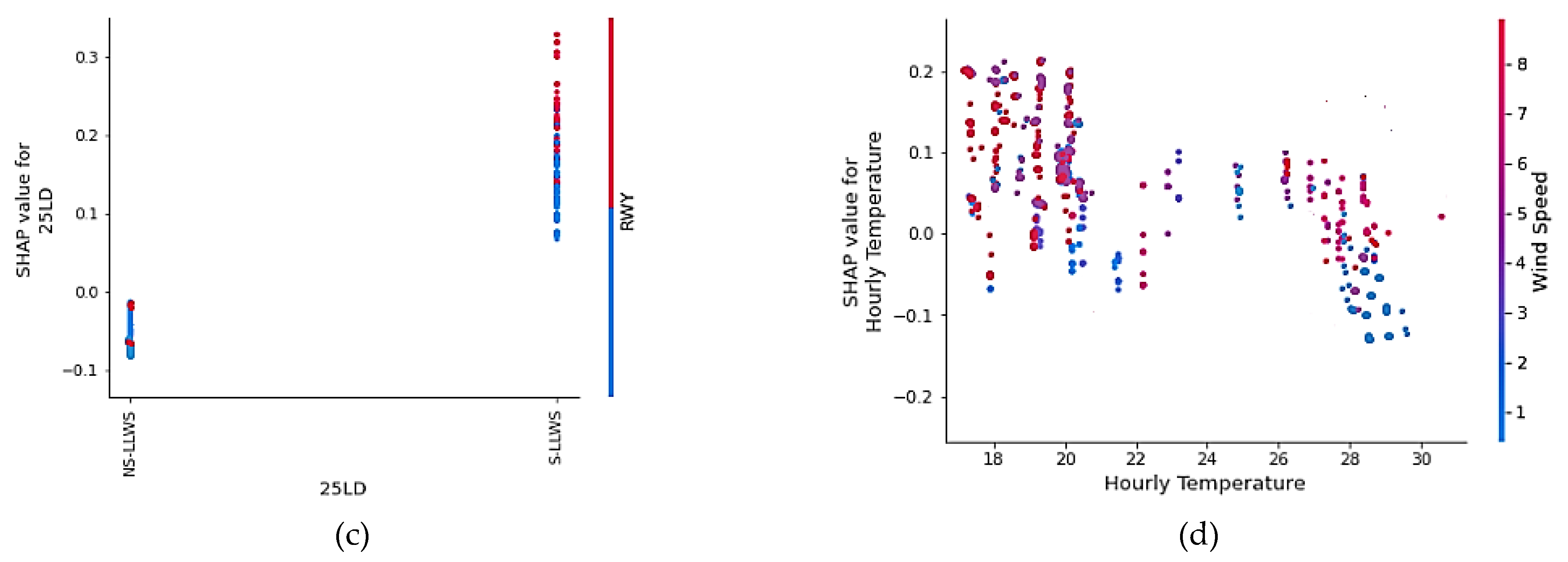
3.3.3. Factor Interaction Analysis

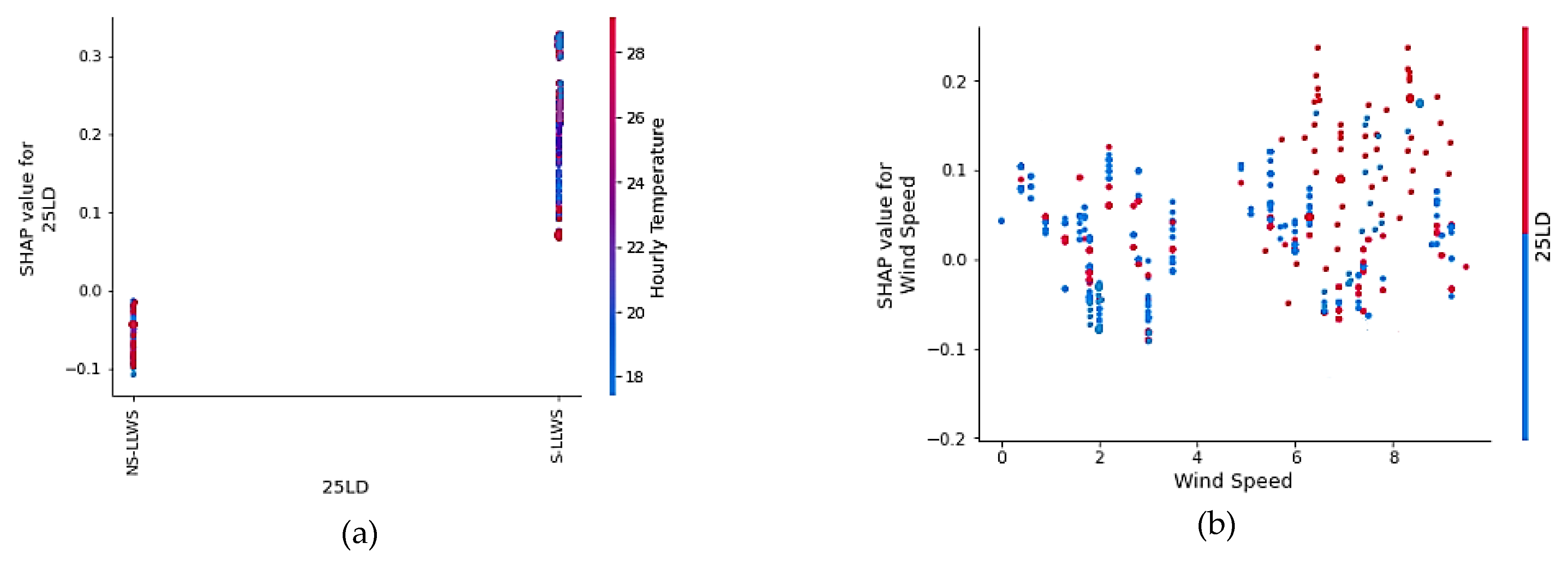
The SHAP interaction plots are examined to identify how the input factors, used to evaluate the SPE framework, interact with one another in terms of their contributions (see Figure 10). The interaction analysis of the top four influential factors, i.e., runway 25LD, hourly temperature, wind speed, and RWY (horizontal location of LLWS occurrence), is provided. Other factors’ interactions, however, could be examined as well. The red and blue scatter plots in Figure 10a depict the variability in the runway 25LD and 25LD SHAP values. When the hourly temperature is low to moderate, the SHAP value for runway 25LD is higher. This means that most of the S-LLWS occurs in the vicinity of runway 25LD when the hourly temperature ranges from low to moderate. The temperature inversion on Hong Kong’s Lantau Island could also be contributing to this scenario.

Figure 10b depicts the distribution of wind speed at runway 25LD. Wind speed points greater than 5 m/s have a higher SHAP value, indicating the likelihood of an S-LLWS event. Figure 10c illustrates that most of the S-LLWS events occurred “on the runway.” The PIREPs reported S-LLWS when aircraft were making their final approach or just when they became airborne after takeoff.

Figure 10d shows that the optimum conditions for the occurrence of S-LLWS were lower than average hourly temperatures and medium-to-high wind speeds. The points representing that scenario fall to the left of the plot and above the SHAP 0.00 reference line. However, to obtain a clear threshold, it may be necessary to know the altitude at which LLWS happen in addition to the parameters that are already known.

4. Conclusions and Recommendations

In this research, a novel SPE framework for the prediction and imbalance classification of LLWS severity has been proposed and compared with tree-based machine learning models, using both treated and untreated HKIA-based LLWS data from LiDAR and PIREPs. The SHAP interpretation system was also used to identify key risk factors and quantify their effects on the occurrence of S-LLWS. In this study, the SPE framework was trained and evaluated using untreated data, whereas both untreated and treated data were used to train the LGBM, AdaBoost, and CART machine learning models. The SMOTE-ENN technique was used as a treatment technique for highly imbalanced LLWS data. In terms of precision, recall, G-Mean, and MCC, the experimental results demonstrated that the SPE framework, based on the untreated data, outperforms all other tree-based models. The newly introduced SPE framework model offers a viable option for modeling and predicting LLWS severity based on imbalanced LLWS data.

Machine learning models, on the other hand, are regularly chastised for their lack of transparency and interpretability. Despite the fact that machine learning models are more adaptable and efficient than statistical approaches, their widespread recognition in the engineering domain continues to be a challenge. To tackle the SPE framework’s interpretability issue, the SHAP interpretation system was used to evaluate the SPE’s output in order to identify major risk factors and assess their impact on the severity of the LLWS. The results of the SHAP interpretation system can be used to rank the risk factor’s overall significance. It can also be used to look into the individual and interaction effects of risk factors (for instance, how specific effects alter in response to changes in the risk factor’s value). The analysis revealed that runway 25LD, hourly temperature, wind speed, and RWY (location of LLWS occurrence) were the top four most significant factors in predicting LLWS severity. The optimistic projections for the occurrence of S-LLWS events were low-to-medium temperatures at runway 25LD with relatively moderate-to-high wind speeds. Likewise, most of the S-LLWS events happen on the runway.

This research outlines a strategy that can be used to conduct a large-scale analysis of LLWS in aviation and serves as a useful tool for aviation policymakers and air traffic safety researchers. This paper discussed the SPE framework using highly imbalanced LLWS data and the SHAP interpretation system. Additional research could be conducted by combining a number of other machine learning techniques with a number of additional risk factors, including monthly variation, location of occurrence of LLWS above ground level, etc. Future research could be expanded by employing additional techniques for augmenting data to deal with highly imbalanced LLWS data.