Impacts of Observed Extreme Antarctic Sea Ice Conditions on the Southern Hemisphere Atmosphere

Abstract

The Antarctic sea ice has undergone dramatic changes in recent years, with the highest recorded sea ice extent in 2014 and the lowest in 2017. We investigated the impacts of the observed changes in these two extremes of Antarctic sea ice conditions on the atmospheric circulation in the Southern Hemisphere. We conducted three numerical simulations with different seasonal cycles of Antarctic sea ice forcings using the Community Atmosphere Model Version 5: the maximum sea ice extent in 2014 (ICE_14), the minimum sea ice extent in 2017 (ICE_17), and the average sea ice extent between 1981 and 2010 (ICE_clm, reference simulation). Our results suggest that the atmospheric response in the Southern Hemisphere showed strong seasonal variations and the atmospheric circulation in winter was more sensitive to the decreased Antarctic sea ice in 2017 than the increased sea ice in 2014. In ICE_14, the westerlies over the polar region were enhanced in summer, but there was no significant change in the zonal-averaged wind in winter. In contrast, in ICE_17, there was a clear equatorward shift in the subtropical jet in winter, but no significant change in summer. The temperature responses were limited to the Antarctic coast, where there were changes in the sea ice in ICE_14 and ICE_17. The warming on the coast of the Amundsen Sea in summer led to a slight increase in precipitation in both simulations.

1. Introduction

The impacts of sea ice changes in the polar region on global climate have attracted increasing attention in recent years, particularly the changes in Arctic sea ice as a result of global warming. In contrast with the substantial decreasing trend in the annual-mean extent of Arctic sea ice in recent decades [1,2,3,4,5], the annual-mean Antarctic sea ice extent (SIE) showed a moderate but significant trend of increase from 1979 to 2014, but then decreased at an abnormal rate, reaching the lowest extent since the late 1970s (when accurate satellite observations of polar sea ice began) in 2017 [6,7,8]. Several possible reasons have been proposed for the sudden decrease in the Antarctic SIE after 2014 including the influence of the extreme El Niño event and the negative phase of the Southern Annular Mode (SAM), a positive zonal wave number three index, wind forcing around Antarctica, and strengthened convective activity around tropical India and the West Pacific [9,10,11,12]. Previous studies have shown that the sea ice changes can affect the atmospheric circulation. The influence of the loss of Arctic sea ice on the weather and climate at high and mid-latitudes in the Northern Hemisphere has been well-discussed [2,3,13]. However, the impacts of changes in Antarctic sea ice on the atmosphere in the Southern Hemisphere have been less well-studied and are controversial.

Associated with historical changes in Antarctic sea ice, Raphael et al. [14] showed that positive sea ice anomalies in the austral summer tended to result in a positive SAM and vice versa. The Southern Hemisphere mid-latitude jet has tended to shift poleward during winter with the expansion of sea ice in recent decades [15]. According to the projections in the CMIP6 models, Antarctic sea ice will decrease toward the end of this century in all the shared socioeconomic pathways [16]. A few studies have examined the impacts of future decreases in Antarctic sea ice on atmosphere in the Southern Hemisphere, but the results are controversial. Menéndez et al. [17] and Bader et al. [18] suggested an equatorward shift in the Southern Hemisphere mid-latitude jet in winter, whereas Kidston et al. [19] found no significant change in the jet in response to a shrinking of SIE. More recently, England et al. [20] showed an equatorward shift of atmospheric jet in the Southern Hemisphere in winter using the CESM-WACCM model. Ayres et al. [21] found both weakening and an equatorward shift of the eddy-driven jet in response to Antarctic sea ice loss, especially in fully coupled models. In contrast, Ayres and Screen [22] showed that the Southern Hemisphere eddy-driven jet tended to weaken rather than drift toward the equator through the simulations of 11 models involved in CMIP5.

Previous studies have mainly focused on the impacts of past and future long-term changes in Antarctic sea ice. In this study, we focused on the impacts of the observed extremes in Antarctic sea ice. From 2014 to 2017, the extent of Antarctic sea ice changed from a record high in 2014 to a record low in 2017 over a short time period. The question is whether these two extreme conditions of Antarctic sea ice have had detectable impacts on the climate in the Southern Hemisphere. This has not been explored in previous studies. Such extreme changes in Antarctic sea ice may occur in the future, so it is necessary to explore the effects of these extreme sea ice conditions. We used the Community Atmosphere Model Version 5 (CAM5) to investigate the atmospheric response in the Southern Hemisphere to the extreme Antarctic sea ice conditions in 2014 and 2017 and analyzed the atmospheric responses in both the austral summer and winter.

2. Data and Methods

We analyzed the atmospheric general circulation model (AGCM) simulations performed with the CAM5 developed by the National Center for Atmospheric Research (NCAR). CAM5 has been widely used in previous studies [5,23]. More detailed information about this model is documented in Neale et al. [24] and Ghan et al. [25]. We ran CAM5 at a horizontal resolution of 1.9° latitude × 2.5° longitude (f19_f19), with 30 vertical levels.

We used the merged Hadley–Optimal Interpolation (OI) sea surface temperature (SST) dataset [26,27] and the bootstrap sea ice concentration (SIC) from the National Snow and Ice Data Center [28] to explore the response of the Southern Hemisphere atmosphere to the prescribed extreme Antarctic sea ice conditions. The Hadley–OI dataset is a combination of the HadISST1 [27] and NOAA OI.v2 [29] datasets and was specifically developed as surface forcing for the uncoupled CAM (see [26] for details).

Figure 1a shows the annual-mean Antarctic SIE from 1979 to 2021. The Antarctic SIE reached a record maximum in 2014 and then decreased sharply in the following years, reaching a record minimum in 2017; the difference in sea ice area between these two extremes is about 2 million square kilometers. To investigate the impact of such extreme sea ice conditions on the atmosphere in the Southern Hemisphere, we performed three model experiments (one control run and two sensitivity experiments). All the simulations were forced by repeating the seasonal cycle of the SST and the SIC. Other forcings such as greenhouse gases and ozone were fixed at the levels in the year 2000. For the control run (ICE_clm), the SST and SIC forcings were averaged over the time period 1981–2010. The two sensitivity experiments (ICE_14 and ICE_17) were conducted with the Antarctic SIC forcings replaced by those for 2014 and 2017, respectively. It is worth noting that the magnitude of the anomalies of Antarctic sea ice forcing in ICE_14 and ICE_17 were not symmetrical, with larger sea ice forcing anomaly in ICE_14 than in ICE_17 (Figure S1a).

Figure 1b–g shows the spatial distribution of the Antarctic SIC. Compared with the climatological sea ice state (Figure 1b), there was increased sea ice cover around Antarctica in ICE_14 in summer, except in the Amundson Sea (Figure S1b). In contrast, there was decreased sea ice cover in the eastern Ross Sea, the Amundson Sea, and the east Weddell Sea in ICE_17 in summer (Figure S1d). In winter, the anomalous sea ice cover mainly occurred in the sea ice margin area, mostly positive in ICE_14 (Figure S1c), but negative in ICE_17 (Figure S1e). All of the simulations were integrated for 71 years and we chose the last 70 years for analysis. A two-tailed Student’s t-test was used to test the significance.

3. Results

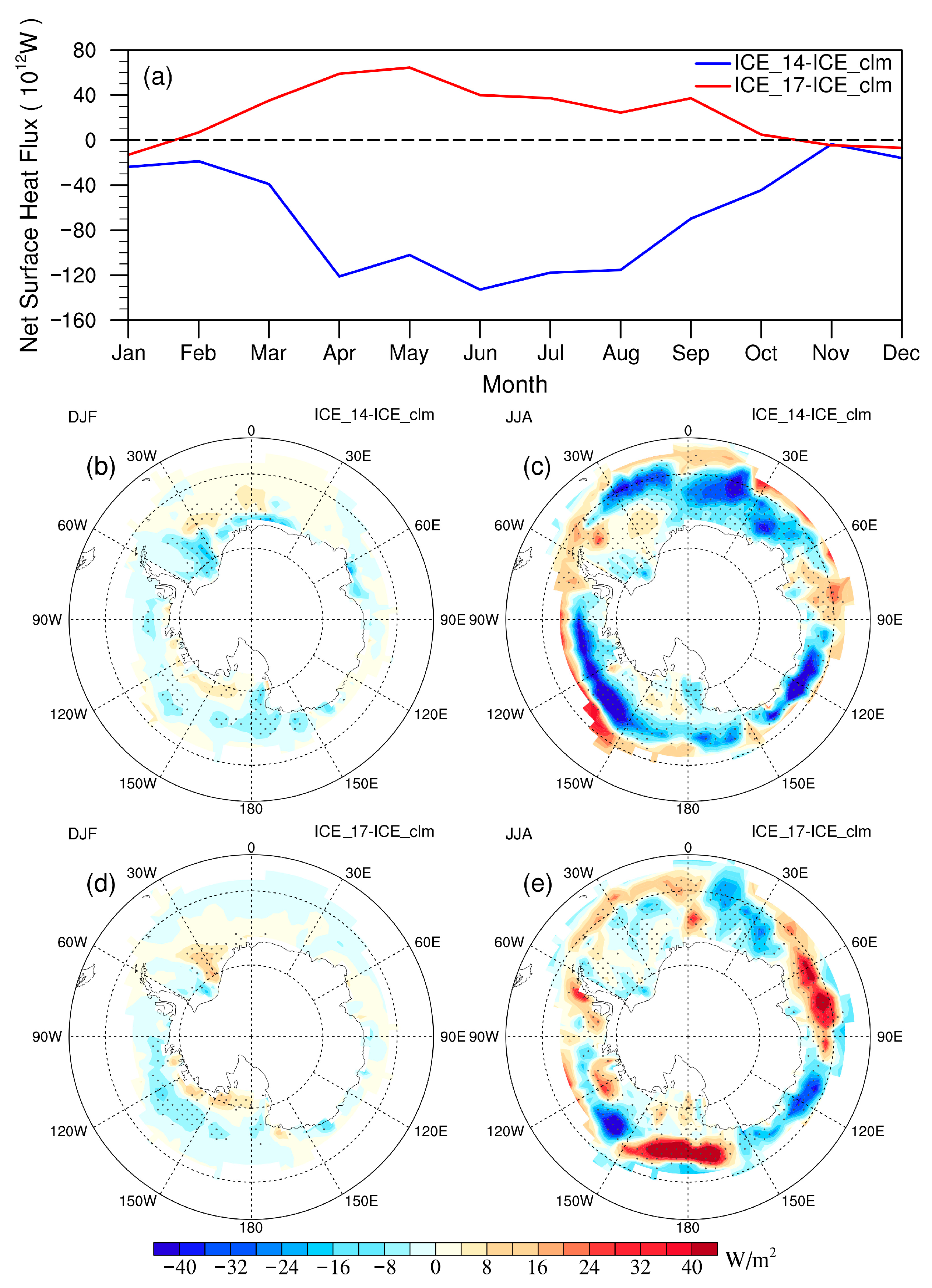
3.1. Surface Heat Flux

As the underlying surface of the atmosphere, variations in Antarctic sea ice can affect the atmosphere by changing the net surface heat fluxes. We calculated the net surface heat flux to the atmosphere as the sum of the latent heat flux, the sensible heat flux, and the longwave flux over areas where the SIC changed. Figure 2a shows the changes in the seasonal net surface heat forcing. Relative to ICE_clm, the increased sea ice cover in ICE_14 resulted in a decreased heat flux from the ocean to the atmosphere, whereas the decreased sea ice cover in ICE_17 resulted in an increased heat flux. The change in the surface heat flux in ICE_14 was about two times larger than that in ICE_17. This is consistent with the larger sea ice anomalies in ICE_14 relative to ICE_clm than those in ICE_17 (Figure S1a). For both ICE_14 and ICE_17, the sensible and latent heat fluxes dominated the change in the net surface forcing (Figure S2a–c). The difference in net surface forcing reached a maximum in the austral autumn and winter as a result of the more significant zonal wind, specific humidity, and temperature gradients between the atmosphere and the ocean [30]. This was also seen from the spatial distribution of the seasonal mean net surface heat flux anomaly (Figure 2b–e). The heat flux anomaly was small in summer and limited to the Weddell Sea, the Amundsen Sea, and the Ross Sea in both experiments (Figure 2b,d). In winter, the heat flux anomaly was significantly enlarged around Antarctica, with the largest anomaly (about ±80 W/m²) over the marginal sea ice zone in both experiments (Figure 2c,e). Based on the difference in the response of the net surface heat flux to changes in SIC in summer and winter, we analyzed the atmospheric responses in the austral summer (December, January, February) and winter (June, July, August).

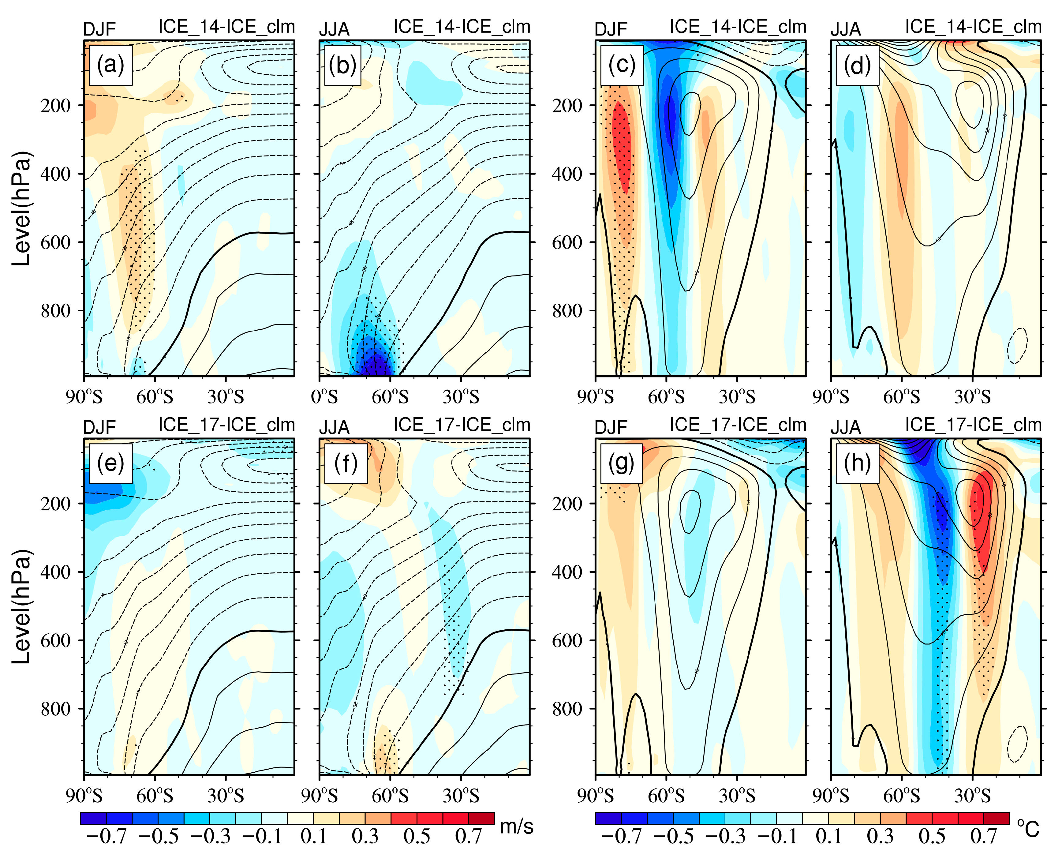
3.2. Response of the Jet Stream

Figure 3 shows the changes in the zonal mean temperature and zonal winds due to changes in sea ice. For ICE_ 2014, there was weak, but significant, cooling in the lower troposphere at high latitudes (Figure 3a) as a result of the decreased surface heat flux upward toward the atmosphere (Figure 2b), accompanied by significant warming in the mid-troposphere (about 850–350 hPa) between about 60° and 70° S (Figure 3a). The westerlies over the polar regions (centered at about 80° S) were significantly strengthened due to the increased temperature gradient toward to the pole, and slightly weakened around 60° S. In winter, the decreased net surface heat flux (Figure 2c) led to intensified cooling between about 55° and 75° S in the lower troposphere (from the surface to about 800 hPa). The increased meridional temperature gradient at about 60° S caused by this cooling strengthened the northerlies and the Ferrell cell (Figure 4b) and gave rise to stronger westerlies in the mid-troposphere (centered at about 60° S), but they were not statistically significant (Figure 3d).

For ICE_17, there was no change in the zonal mean of the temperature and the zonal wind in summer (Figure 3e,g) and no change in the three-cell circulation (Figure 4c). In winter, there was significant warming in the lower troposphere between about 55° and 65° S (Figure 3f), but the intensity was weaker than the cooling in ICE_14. There was a small, but significant amount of cooling in the mid-troposphere around 30° S in winter. The decreased temperature gradient from the subtropics to the pole weakened the westerlies south of 30° S and the increased temperature gradient from the tropics to the subtropics strengthened the westerlies north of 30° S in the mid- to upper troposphere (Figure 3f). This suggests an equatorward shift in the subtropical jet, corresponding to a weakened Ferrell cell and a contracted Hadley cell (Figure 4d). In contrast to the results from previous atmospheric models showing non-significant responses to decreasing Antarctic sea ice [19] or responses that were constrained to mid- and high latitudes [20], our model showed significant changes in the subtropical zonal winds in winter.

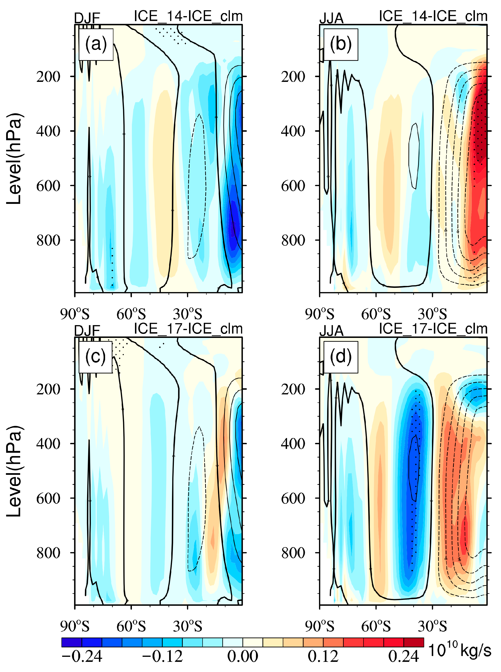
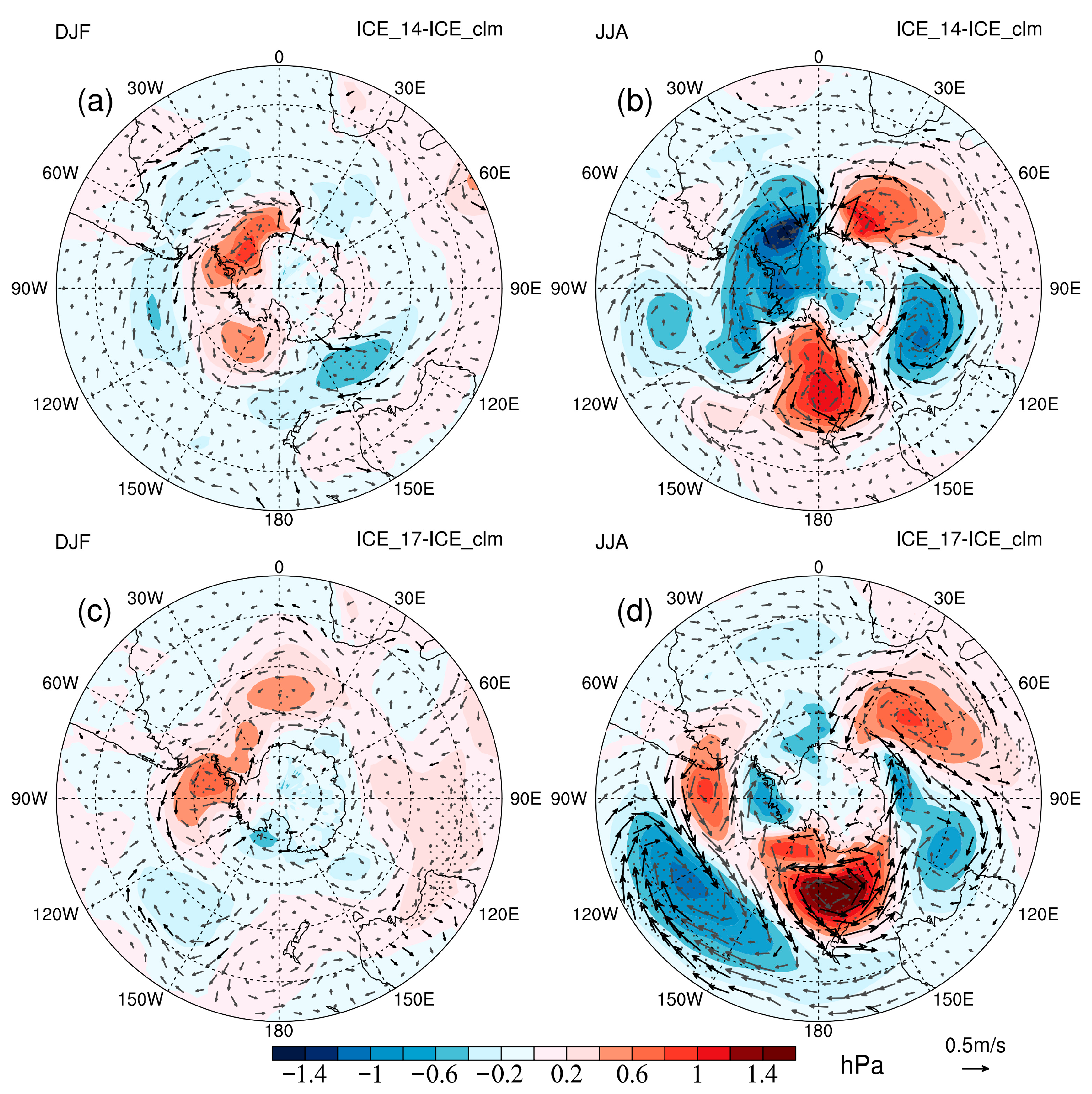
3.3. Changes in the Circulation in the Lower and Mid-Troposphere

Figure 5 shows the changes in sea-level pressure and near-surface winds resulting from the extreme sea ice conditions. ICE_14 produced above-normal pressure over the Weddell Sea in summer (Figure 5a). As the height increased, there was above-normal pressure over the Bellingshausen Sea at 500 hPa (Figure S3a). There was a negative phase of SAM (not significant) at both the surface and at 500 hPa. This was consistent with an easterly anomaly centered at about 60° S (Figure 5a and Figure S3a). In contrast, the responses in winter were zonal asymmetry and a wavenumber 2 pattern in both the lower and mid-troposphere between about 40° and 70° S. There was below-normal pressure in the Amundsen and Weddell Seas, above-normal pressure to the south of Africa and in the southwestern Indian Ocean, below-normal pressure in the southeastern Indian Ocean and south of Australia, and above-normal pressure in the Southwestern Pacific (Figure 5b and Figure S3b). This zonal asymmetry resulted in no significant change in the zonal-averaged zonal wind as a result of compensating responses.

There was above-normal pressure over the Bellingshausen Sea for ICE_17 in summer (Figure 5c). As the height increased, above-normal pressure was seen over the Amundsen Sea at 500 hPa (Figure S3c). In contrast, the responses in winter were zonally asymmetrical. The southwestern Indian Ocean and southwestern Pacific Ocean between 45° and 70° S were dominated by above-normal pressure anomalies, whereas the subtropical region of the southern Pacific was dominated by below-normal pressure anomalies (Figure 5d and Figure S3d). Consistently, there were westerly wind anomalies in the north of 30° S and an easterly wind anomaly at about 45° S over the Pacific region, which resulted in an equatorward shift in the subtropical high. Although the anomaly of the sea ice forcing field and the surface heat flux anomaly in ICE_17 were smaller than those in ICE_14, the anomaly in the response of the circulation in ICE_14 was limited to mid- and high latitudes, whereas the anomaly in the response of the circulation in ICE_17 reached the subtropic. This may indicate that the climate in the Southern Hemisphere is more sensitive to a loss of Antarctic sea ice than to an increase in sea ice.

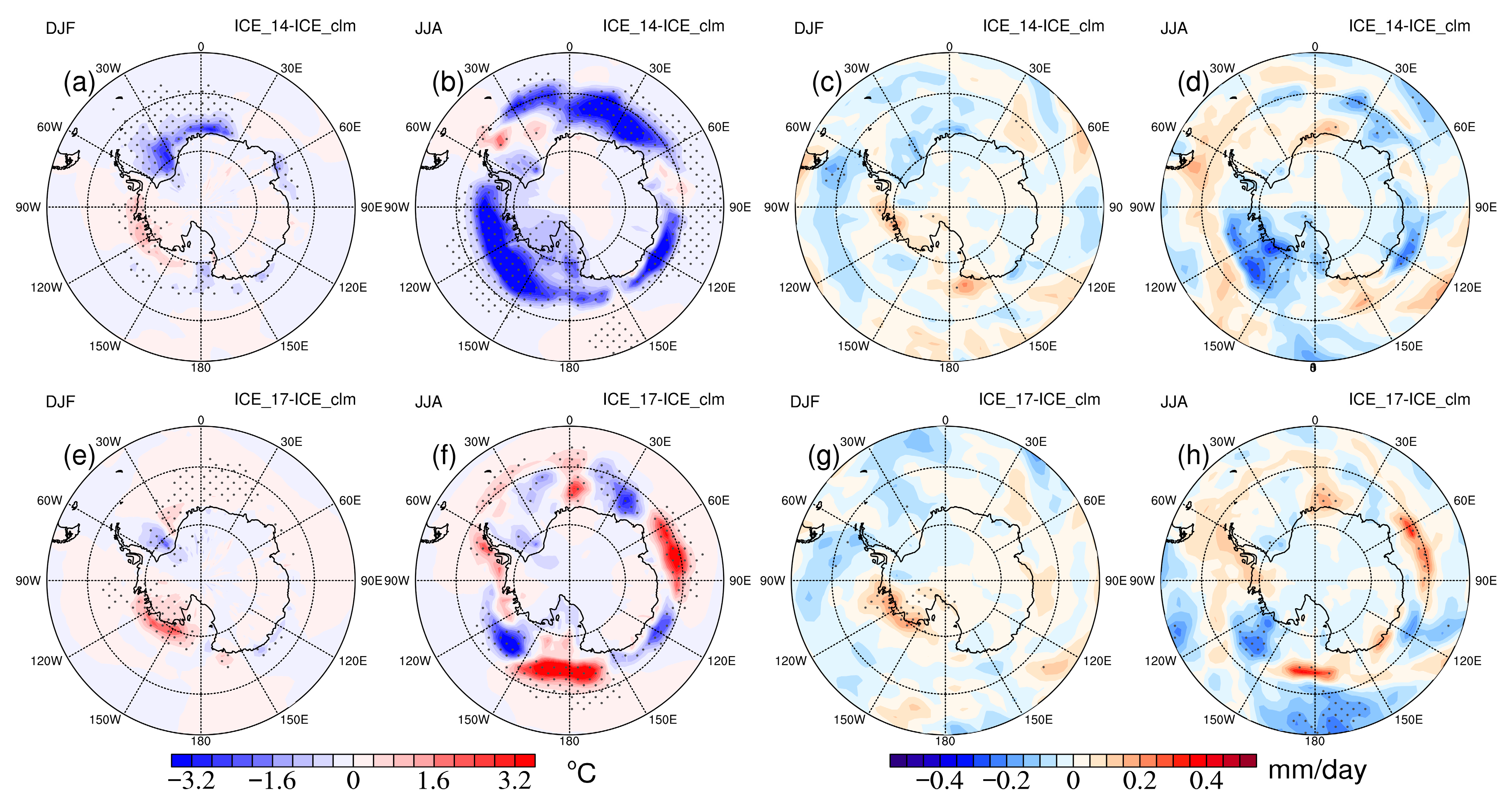
3.4. Changes in Temperature and Precipitation

The temperature changes in both ICE_14 and ICE_17 were largely confined to high latitudes, especially in the area adjacent to changes in sea ice forcing (Figure 6a–d). The increased sea ice in 2014 led to a small, but significant amount of warming in the Amundsen Sea and adjacent continents, but moderate cooling in the Weddell Sea and along the coastal ocean of the eastern Antarctica in summer (Figure 6a). In winter, there was a broad region of cooling along the Antarctic coast associated with the increase in sea ice. The continental areas along the coasts of the eastern Ross and Amundsen Seas also showed significant cooling as a result of the southern wind anomaly, which brought cold air from Antarctica (Figure 5b and Figure 6b). In ICE_17, significant warm anomalies were found on the coast of the eastern Ross and Amundsen Seas in summer (Figure 6e). This was consistent with the increased surface heat flux (Figure 2d) and the north wind anomaly (Figure 5c), which both bring warmer air from the Amundsen Sea. In winter, despite the stronger surface heat flux anomaly than in summer, the temperature changes were confined to the coastal ocean of Antarctica; there was no significant change in temperature over the Antarctic continent (Figure 6f).

Consistent with the warming and north wind anomaly on the coast of the Amundsen Sea in summer, there was slightly increased precipitation on the coast of the Amundsen Sea in ICE_14 (Figure 6c). In winter, the south wind anomaly on the coast of the Amundsen Sea (Figure 5b) brought cold, dry air from the central Antarctic to the coast, resulting in significantly decreased precipitation over the Amundsen Sea (Figure 6d). In ICE_17, there was significantly increased precipitation on the coasts of the Amundsen Sea in summer (Figure 6g) as a result of the northerly wind anomaly bringing warm, moist air from the ocean (Figure 5c). In winter, changes in precipitation mainly occurred over the ocean and there was no significant change in precipitation over Antarctica (Figure 6h). The changes in precipitation were dominated by changes in snowfall (Figure S4). In response to the decreased amount of sea ice in 2017, there was a significant increase in snowfall on the coast of the Amundsen and eastern Ross seas. This increased snowfall increased the mass input and may influence the ice sheet balance in these regions.

4. Conclusions and Discussion

We explored the impacts of extreme sea ice conditions in Antarctica on the Southern Hemisphere summer and winter climate by forcing CAM5 with the seasonal cycle of the average Antarctic SIC from 1981 to 2010 and the Antarctic SIC in 2014 and 2017. Our results show that the extreme Antarctic sea ice conditions in 2014 and 2017 might have affected the tropospheric jets in the Southern Hemisphere. The large responses of temperature and precipitation were largely limited to high latitudes.

The increased Antarctic sea ice in 2014 may have led to enhanced westerlies over the polar region, accompanied by zonal-averaged warming between about 60° and 70° S in the mid-troposphere and warming and increased precipitation on the coasts of the Amundsen Sea in summer. In winter, there was significant cooling around Antarctica and slightly decreased precipitation over the Amundsen Sea. The extremely low Antarctic sea ice in 2017 resulted in significant warming and increased precipitation on the coasts of the eastern Ross Sea and the Amundsen Sea in summer and an equatorward shift in the subtropical jet in winter. Compared with Antarctic sea ice forcing in ICE_clm, the sea ice forcing anomaly in ICE_14 was stronger than that in ICE_17. However, the impacts of the sea ice forcing anomaly in ICE_17 on the atmospheric circulation in the Southern Hemisphere reached as far as the subtropics, whereas the response in ICE_14 was limited to mid- and high latitudes. This suggests that the climate of the Southern Hemisphere was more sensitive to the decreased Antarctic sea ice in 2017 than the increased sea ice in 2014.

We also compared the effects of extreme changes in sea ice on the climate of the Southern Hemisphere in previous studies (

Table 1. Previous studies that have explored the impacts of Antarctic sea ice changes on the Southern Hemisphere.

Reference	Model	Conclusion
Kidston et al. [19]	Community Atmosphere Model (CAM3)	The mid-latitude jet shifts poleward when sea ice extent increased during winter.
Raphael et al. [14]	Community Climate System Model Version Three (CCSM3)	The polar cell expands (contracts) under minimum (maximum) sea ice conditions; the Southern Hemisphere Annular Mode tends to be negative (positive) when the sea ice is at a minimum (maximum) in summer.
Bader et al. [18]	atmospheric general circulation model ECHAM5	The mid-latitude jet and the storm tracks shift equatorward and there is a negative phase of the Southern Hemisphere Annular Mode under future decreased sea ice conditions.
Smith et al. [15]	Met Office Hadley Centre global climate model HadGEM3	Both the atmospheric-only and coupled experiments simulate a poleward shift of mid-latitude jet under increased sea ice condition in recent years, especially in the cold seasons.
England et al. [20]	Whole Atmosphere Coupled Climate Model (WACCM)	Future losses of Antarctic sea ice will act to shift the tropospheric jet equatorward in the cold seasons. The response of the surface temperature and precipitation is limited to the southern high latitudes, but is unable to impact the interior of the Antarctic continent.

). Raphael et al. [14] conducted numerical experiments using the coupled NCAR Community Climate System Model Version Three. They used the monthly SIC from 1978 to 2000 to select the months with the maximum and minimum SIC in each of 12 months as the forcings in sensitivity experiments. Their results showed a positive SAM in response to the maximum SIC and a negative SAM in response to the minimum SIC in summer. In contrast, our results indicate a slightly negative SAM in response to the increased sea ice in 2014 and no change in the SAM in response to the decreased sea ice in 2017. This difference might result from air–ocean coupling. England et al. [20,31,32] showed that the response to losses of Antarctic sea ice were limited to the mid- and high latitudes of the Southern Hemisphere in the Whole Atmosphere Community Climate Model (WACCM), but it may extend to the tropics and even the Northern Hemisphere in the coupled model. This again shows the importance of the air–ocean coupling.

Kidston et al. [19] used the poleward contraction and equatorial expansion of the climatological Antarctic sea ice by 7° of latitude as the forcing fields for their sensitivity experiments. Smith et al. [15] investigated the impacts of the long-term observed trends in the Antarctic sea ice long-term trend. Both sets of results showed a poleward shift of the mid-latitude jet in winter as a response to increased Antarctic sea ice in the atmospheric-only model. In contrast, our results showed no significant change in the mid-latitude jet.

Bader et al. [18] and England et al. [20] explored the effects of future losses of Antarctic sea ice at the end of the 21st century using an atmospheric-only model and suggested a equatorward shift of the mid-latitude jet in winter in response to sea ice loss. However, our results showed no significant change in the mid-latitude jet, but an equatorward shift of the subtropical jet in winter in response to the extremely low sea ice in 2017. The large differences in the forcing field between our ICE_17 experiment and the sensitivity experiments of Bader et al. [18] and England et al. [20] may have resulted in this low comparability. In terms of temperature and precipitation, consistent with England et al. [20], sea ice loss in 2017 caused significant near-surface warming on the coasts of Antarctica, but this warming did not penetrate inland to the Antarctic continent. These earlier studies conducted similar numerical experiments to ours, but we used a different model with different forcings for the Antarctic sea ice. The comparison of our results with previous studies suggest that the influence of Antarctic sea ice is sensitive to both the adopted model and the distribution of sea ice forcing anomalies.

References

1. Gao, Y.Q.; Sun, J.Q.; Li, F.; He, S.P.; Sandven, S.; Yan, Q.; Zhang, Z.S.; Lohmann, K.; Keenlyside, N.; Furevik, T.; et al. Arctic Sea Ice and Eurasian Climate: A Review. Adv. Atmos. Sci. 2015, 32, 92–114. [Google Scholar] [CrossRef] [Green Version]
2. Cohen, J.; Screen, J.A.; Furtado, J.C.; Barlow, M.; Whittleston, D.; Coumou, D.; Francis, J.; Dethloff, K.; Entekhabi, D.; Overland, J.; et al. Recent Arctic amplification and extreme mid-latitude weather. Nat. Geosci. 2014, 7, 627–637. [Google Scholar] [CrossRef] [Green Version]
3. Liu, J.P.; Curry, J.A.; Wang, H.J.; Song, M.R.; Horton, R.M. Impact of declining Arctic sea ice on winter snowfall. Proc. Natl. Acad. Sci. USA 2012, 109, 4074–4079. [Google Scholar] [CrossRef] [PubMed] [Green Version]
4. Petoukhov, V.; Semenov, V.A. A link between reduced Barents-Kara sea ice and cold winter extremes over northern continents. J. Geophys. Res.-Atmos. 2010, 115, D21111. [Google Scholar] [CrossRef]
5. Song, M.R.; Wang, S.Y.; Zhu, Z.; Liu, J.P. Nonlinear changes in cold spell and heat wave arising from Arctic sea-ice loss. Adv. Clim. Chang. Res. 2021, 12, 553–562. [Google Scholar] [CrossRef]
6. Eayrs, C.; Li, X.C.; Raphael, M.N.; Holland, D.M. Rapid decline in Antarctic sea ice in recent years hints at future change. Nat. Geosci. 2021, 14, 460–464. [Google Scholar] [CrossRef]
7. Parkinson, C.L. A 40-y record reveals gradual Antarctic sea ice increases followed by decreases at rates far exceeding the rates seen in the Arctic. Proc. Natl. Acad. Sci. USA 2019, 116, 14414–14423. [Google Scholar] [CrossRef] [Green Version]
8. Turner, J.; Hosking, J.S.; Bracegirdle, T.J.; Marshall, G.J.; Phillips, T. Recent changes in Antarctic Sea Ice. Philos. Trans. R. Soc. A-Math. Phys. Eng. Sci. 2015, 373, 20140163. [Google Scholar] [CrossRef]
9. Schlosser, E.; Haumann, F.A.; Raphael, M.N. Atmospheric influences on the anomalous 2016 Antarctic sea ice decay. Cryosphere 2018, 12, 1103–1119. [Google Scholar] [CrossRef] [Green Version]
10. Wang, Z.M.; Turner, J.; Wu, Y.; Liu, C.Y. Rapid Decline of Total Antarctic Sea Ice Extent during 2014-16 Controlled by Wind-Driven Sea Ice Drift. J. Clim. 2019, 32, 5381–5395. [Google Scholar] [CrossRef]
11. Meehl, G.A.; Arblaster, J.M.; Chung, C.T.Y.; Holland, M.M.; DuVivier, A.; Thompson, L.; Yang, D.X.; Bitz, C.M. Sustained ocean changes contributed to sudden Antarctic sea ice retreat in late 2016. Nat. Commun. 2019, 10, 14. [Google Scholar] [CrossRef] [PubMed] [Green Version]
12. Wang, G.M.; Hendon, H.H.; Arblaster, J.M.; Lim, E.P.; Abhik, S.; van Rensch, P. Compounding tropical and stratospheric forcing of the record low Antarctic sea-ice in 2016. Nat. Commun. 2019, 10, 13. [Google Scholar] [CrossRef] [PubMed] [Green Version]
13. Peings, Y.; Magnusdottir, G. Response of the Wintertime Northern Hemisphere Atmospheric Circulation to Current and Projected Arctic Sea Ice Decline: A Numerical Study with CAM5. J. Clim. 2014, 27, 244–264. [Google Scholar] [CrossRef] [Green Version]
14. Raphael, M.N.; Hobbs, W.; Wainer, I. The effect of Antarctic sea ice on the Southern Hemisphere atmosphere during the southern summer. Clim. Dyn. 2011, 36, 1403–1417. [Google Scholar] [CrossRef]
15. Smith, D.M.; Dunstone, N.J.; Scaife, A.A.; Fiedler, E.K.; Copsey, D.; Hardiman, S.C. Atmospheric Response to Arctic and Antarctic Sea Ice: The Importance of Ocean-Atmosphere Coupling and the Background State. J. Clim. 2017, 30, 4547–4565. [Google Scholar] [CrossRef] [Green Version]
16. Roach, L.A.; Dorr, J.; Holmes, C.R.; Massonnet, F.; Blockley, E.W.; Notz, D.; Rackow, T.; Raphael, M.N.; O’Farrell, S.P.; Bailey, D.A.; et al. Antarctic Sea Ice Area in CMIP6. Geophys. Res. Lett. 2020, 47, e2019GL086729. [Google Scholar] [CrossRef]
17. Menéndez, C.G.; Serafini, V.; Treut, H.L. The effect of sea-ice on the transient atmospheric eddies of the Southern Hemisphere. Clim. Dyn. 1999, 15, 659–671. [Google Scholar] [CrossRef]
18. Bader, J.; Flugge, M.; Kvamsto, N.G.; Mesquita, M.D.S.; Voigt, A. Atmospheric winter response to a projected future Antarctic sea-ice reduction: A dynamical analysis. Clim. Dyn. 2013, 40, 2707–2718. [Google Scholar] [CrossRef] [Green Version]
19. Kidston, J.; Taschetto, A.S.; Thompson, D.W.J.; England, M.H. The influence of Southern Hemisphere sea-ice extent on the latitude of the mid-latitude jet stream. Geophys. Res. Lett. 2011, 38, 5. [Google Scholar] [CrossRef] [Green Version]
20. England, M.R.; Polvani, L.M.; Sun, L. Contrasting the Antarctic and Arctic atmospheric responses to projected sea ice loss in the late 21st Century. J. Clim. 2018, 31, 6353–6370. [Google Scholar] [CrossRef]
21. Ayres, H.C.; Screen, J.A.; Blockley, E.W.; Bracegirdle, T.J. The Coupled Atmosphere-Ocean Response to Antarctic Sea Ice Loss. J. Clim. 2022, 35, 4665–4685. [Google Scholar] [CrossRef]
22. Ayres, H.C.; Screen, J.A. Multimodel Analysis of the Atmospheric Response to Antarctic Sea Ice Loss at Quadrupled CO2. Geophys. Res. Lett. 2019, 46, 9861–9869. [Google Scholar] [CrossRef]
23. Zhang, G.W.; Zeng, G.; Li, C.; Yang, X.Y. Impact of PDO and AMO on interdecadal variability in extreme high temperatures in North China over the most recent 40-year period. Clim. Dyn. 2020, 54, 3003–3020. [Google Scholar] [CrossRef]
24. Neale, R.B.; Gettelman, A.; Park, S.; Conley, A.J.; Kinnison, D.; Dan, M.; Smith, A.K.; Vitt, F.; Morrison, H.; Cameronsmith, P.; et al. Description of the NCAR Community Atmosphere Model (CAM 5.0). NCAR Tech. Note NCAR/TN-486+STR 2010, 1, 1–12. [Google Scholar]
25. Ghan, S.J.; Liu, X.; Easter, R.C.; Zaveri, R.; Rasch, P.J.; Yoon, J.H.; Eaton, B. Toward a Minimal Representation of Aerosols in Climate Models: Comparative Decomposition of Aerosol Direct, Semidirect, and Indirect Radiative Forcing. J. Clim. 2012, 25, 6461–6476. [Google Scholar] [CrossRef]
26. Hurrell, J.W.; Hack, J.J.; Shea, D.; Caron, J.M.; Rosinski, J. A new sea surface temperature and sea ice boundary dataset for the Community Atmosphere Model. J. Clim. 2008, 21, 5145–5153. [Google Scholar] [CrossRef]
27. Rayner, N.A.; Parker, D.E.; Horton, E.B.; Folland, C.K.; Alexander, L.V.; Rowell, D.P.; Kent, E.C.; Kaplan, A. Global analyses of sea surface temperature, sea ice, and night marine air temperature since the late nineteenth century. J. Geophys. Res.-Atmos. 2003, 108, 37. [Google Scholar] [CrossRef] [Green Version]
28. Comiso, J.C. Bootstrap Sea Ice Concentrations from Nimbus-7 SMMR and DMSP SSM/I-SSMIS, Version 3; NASA National Snow and Ice Data Center Distributed Active Archive Center: Boulder, CO, USA, 2017. [CrossRef]
29. Reynolds, R.W.; Rayner, N.A.; Smith, T.M.; Stokes, D.C.; Wang, W.Q. An improved in situ and satellite SST analysis for climate. J. Clim. 2002, 15, 1609–1625. [Google Scholar] [CrossRef]
30. Yu, L.S.; Weller, R.A. Objectively analyzed air-sea heat fluxes for the global ice-free oceans (1981–2005). Bull. Amer. Meteorol. Soc. 2007, 88, 527–540. [Google Scholar] [CrossRef] [Green Version]
31. England, M.R.; Polvani, L.M.; Sun, L. Robust Arctic warming caused by projected Antarctic sea ice loss. Environ. Res. Lett. 2020, 15, 9. [Google Scholar] [CrossRef]
32. England, M.R.; Polvani, L.M.; Sun, L.T.; Deser, C. Tropical climate responses to projected Arctic and Antarctic sea-ice loss. Nat. Geosci. 2020, 13, 275–281. [Google Scholar] [CrossRef]
Figure 1. Extent and concentration of Antarctic sea ice. (a) Annual-mean Antarctic sea ice extent from 1979 to 2021. Antarctic sea ice concentration averaged between 1981 and 2010 in (b) summer and (e) winter. Antarctic sea ice concentration in (c) summer 2014 and (f) winter 2014. Antarctic sea ice concentration in (d) summer 2017 and (g) winter 2017. The orange line in (bg) represents the edge of the sea ice defined as the contour of 15% ice concentration.
Atmosphere 14 00036 g001
Figure 2. Changes in the net surface heat flux (the sum of the latent heat flux, the sensible heat flux, and the longwave flux over all grids where the sea ice changes) as a result of changes in Antarctic sea ice. (a) Difference in the total Antarctic net heat flux between ICE_14 and ICE_clm (blue line) and between ICE_17 and ICE_clm (red line). Spatial difference between ICE_14 and ICE_clm in the austral (b) summer and (c) winter. Spatial difference between ICE_17 and ICE_clm in the austral (d) summer and (e) winter. Positive means an upward flux from the ocean to the atmosphere. The dotted areas were statistically significant at the 95% confidence level.
Atmosphere 14 00036 g002
Figure 3. Changes in the zonal mean temperature and zonal winds as a result of changes in Antarctic sea ice. The zonal mean temperature (a,e) in summer and (b,f) in winter. The zonal mean zonal wind in (c,g) summer and (d,h) winter. Parts (ad) show the differences between ICE_14 and ICE_clm; (eh) show the differences between ICE_17 and ICE_clm. The dotted areas were statistically significant at the 95% confidence level. The contours represent the mean state of ICE_clm.
Atmosphere 14 00036 g003
Figure 4. Changes in the zonal mean atmospheric meridional stream function as a result of changes in Antarctic sea ice. Differences between ICE_14 and ICE_clm in (a) summer and (b) winter. Differences between ICE_17 and ICE_clm in (c) summer and (d) winter. The dotted areas were statistically significant at the 95% confidence level. The contours represent the mean state of ICE_clm.
Atmosphere 14 00036 g004
Figure 5. Changes in the sea-level pressure and near-surface winds as a result of changes in Antarctic sea ice. Differences between ICE_14 and ICE_clm in (a) summer and (b) in winter. Differences between ICE_17 and ICE_clm in (c) summer and (d) winter. The dotted areas were statistically significant at the 95% confidence level. The contours represent the mean state of ICE_clm.
Atmosphere 14 00036 g005
Figure 6. Changes in the 2-m temperature and precipitation as a result of changes in Antarctic sea ice. Temperature responses of ICE_14 in (a) summer and (b) winter. Precipitation responses of ICE_14 in (c) summer and (d) winter. Temperature responses of ICE_17 in (e) summer and (f) winter. Precipitation responses of ICE_17 in (g) summer and (h) winter. Dotted areas indicate statistical significance at the 95% confidence level.
Atmosphere 14 00036 g006