Article

Prediction and Interpretation of Low-Level Wind Shear Criticality Based on Its Altitude above Runway Level: Application of Bayesian Optimization–Ensemble Learning Classifiers and SHapley Additive exPlanations

1
The Key Laboratory of Infrastructure Durability and Operation Safety in Airfield of CAAC, Tongji University, 4800 Cao’an Road, Jiading, Shanghai 201804, China
2
Hong Kong Observatory, 134A Nathan Road, Kowloon, Hong Kong, China
3
Shanghai Research Center for Smart Mobility and Road Safety, Shanghai 200092, China
*
Author to whom correspondence should be addressed.
Atmosphere 2022, 13(12), 2102; https://doi.org/10.3390/atmos13122102
Submission received: 8 November 2022 / Revised: 27 November 2022 / Accepted: 12 December 2022 / Published: 15 December 2022
(This article belongs to the Special Issue Advances in Transportation Meteorology)

Abstract

:
Low-level wind shear (LLWS) is a rare occurrence and yet poses a major hazard to the safety of aircraft. LLWS event occurrence within 800 feet of the runway level are dangerous to approaching and departing aircraft and must be accurately predicted. In this study, first the Bayesian Optimization–Ensemble Learning Classifiers (BO-ELCs) including Adaptive Boosting, Light Gradient Boosting Machine, Categorical Boosting, Extreme Gradient Boosting, and Random Forest were trained and tested using a dataset of 234 LLWS events extracted from pilot flight reports (PIREPS) and weather reports at Hong Kong International Airport. Afterward, the SHapley Additive exPlanations (SHAP) algorithm was utilized to interpret the best BO-ELC. Based on the testing set, the results revealed that the Bayesian Optimization–Random Forest Classifier outperformed the other BO-ELCs in accuracy (0.714), F1-score (0.713), AUC-ROC (0.76), and AUR-PRC (0.75). The SHAP analysis found that the hourly temperature, wind speed, and runway 07LA were the top three crucial factors. A high hourly temperature and a moderate-to-high wind speed made Runway 07LA vulnerable to the occurrence of critical LLWS events. This research was a first attempt to forecast the criticality of LLWS in airport runway vicinities and will assist civil aviation airport authorities in making timely flight operation decisions.

1. Introduction

Globally, the civil aviation industry has grown rapidly in the last decade as a consequence of enhanced economic development. Passenger traffic worldwide surpassed 8.8 billion in 2018 and is expected to triple to 10 billion by 2037. It is projected to grow at a 3.7% annual rate in the long run and reach 19.7 billion by 2040 [1]. Although there is a boom in the aviation industry worldwide, weather is one of the key factors that has a major impact on overall airline operations. It is a significant contributor to flight cancellations, delays, and—in the worst-case scenario—accidents. Wind shear is an aviation term that refers to a sudden, abrupt change in wind direction or speed, whereas low-level wind shear (LLWS) refers to wind shear that occurs below 1600 feet (500 m) above ground level (AGL). Low-level jet streams, frontal systems, low-level temperature inversions, and LLWS are closely associated, more specifically with the unique wind-shear conditions created by man-made structures such as the distribution of various buildings, terrain roughness, and natural obstructions such as mountains and water/land interfaces, among other factors, at and around a particular airport [2].

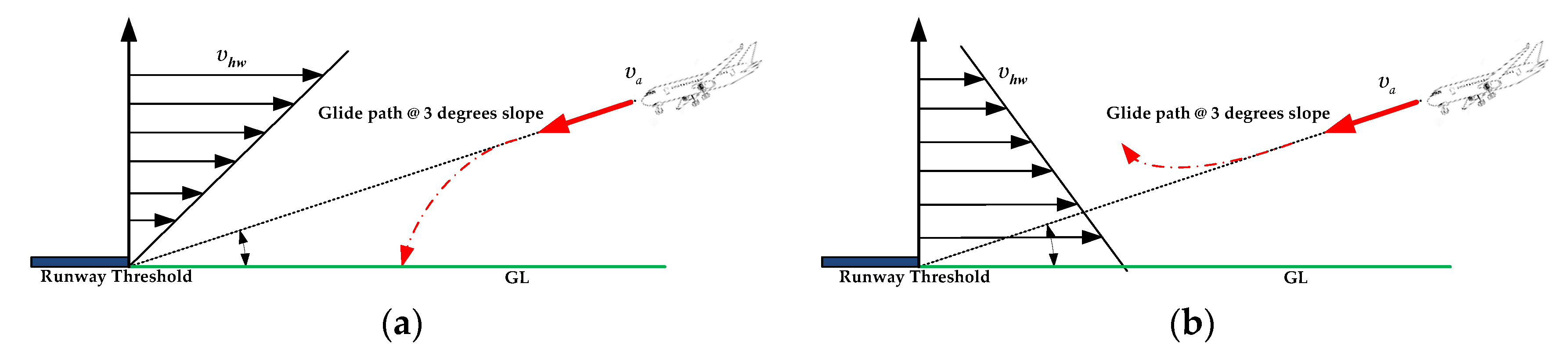
1.1. Low-Level Wind Shear: Pilots’ Invisible Enemy

The cockpit remains extremely active during the landing phase, and the captain and co-pilot must make a number of quick decisions to complete their landing checklist. However, poor weather conditions, complex terrain, and the presence of buildings near the airport will increase turbulence along the glide path. Therefore, the occurrence of LLWS below 800 feet above the ground is regarded as the most critical phenomenon for both approaching and departing aircraft. The pilot must contend with violent updrafts and downdrafts as well as abrupt changes in the aircraft’s horizontal and vertical movement while completing the landing checklist. As depicted in Figure 1, this critical condition may lead to a missed approach, landing short of the runway (loss of lift), or deviation from the actual flight path during final approach. Basically, there are two detrimental and potentially hazardous effects of LLWS on approaching aircraft: perturbation of the glide path and deviancy of the approach speed from the established (set) value [3]. As a result, the pilot may perceive additional pressure during the approach phase when the engine power is low and the airspeed is close to stall speed due to unexpected changes in wind direction or speed. This effect of declining and raising headwind shear on an aircraft during an approach is depicted in Figure 2 (assuming no pilot intervention is being used); both scenarios utilize a conventional instrument landing system with a 3-degree glide path and final approach speed ( υ a ) . In the first scenario (Figure 2a), the approaching aircraft is subjected to a declining headwind with the headwind speed ( υ hw ) . As the aircraft approaches the ground, its airspeed (the aircraft’s speed in relation to the surrounding air flow) declines, thereby lowering lift and tending to result in a greater descent angle due to the transient force imbalance. In this scenario, the aircraft may possibly land short of the runway. The second case (Figure 2b) assumes a rising headwind on the same glide path and slope (3 degrees). As a result, the aircraft’s airspeed increases in relation to the surrounding air flow, thereby generating more lift and resulting in a flatter angle of descent or even a climb. In this scenario, landing may possibly be aborted and a go-around initiated.

1.2. Low-Level Wind Shear Detection Technologies

Airports worldwide have profited significantly from the availability of meticulous, high-resolution technologies for remote sensing including Terminal Doppler Weather Radar (TDWR) and Doppler Light Detection and Ranging (LiDAR) [4,5,6]. By far, the most extensively used approaches for detecting wind shear are TDWR, ground-based anemometer networks, and wind profilers. This approach has been shown to be effective in alerting LLWS since the mid-1990s, most notably during the passage of tropical cyclones and thunderstorms. When the weather is clear, the TDWR system does not offer accurate wind information. Certain LLWS incidents, on the other hand, are connected to airflow that reaches the airport from rugged terrain. To deal with these scenarios, a new method of detection that is not dependent on humid conditions must be developed. The LiDAR system has been added as a booster to the TDWR in order to identify and warn of LLWS in clear skies. When the air is clear, Doppler LiDAR can detect return signals from aerosols and offer precise Doppler wind measurements. To ensure the safety of civil aircraft, TDWRs and LiDARs have been extensively installed at major airports worldwide. However, only a few airports worldwide, including Japan, Malaysia, Germany, France, Korea, Singapore, and Hong Kong, possess these LLWS alerting system technologies due to high maintenance and equipment costs, a lack of pertinent research, and specific geographical characteristics [7]. Additionally, these LLWS alerting technologies, which are based on remote sensing and/or on-site measurements, have been demonstrated to be successful and operational. When an LLWS event is detected or observed, these detection- or observation-based technologies send notifications. However, these detection- or observation-based technologies cannot predict when the next LLWS event will occur or what risk factors contribute to its occurrence as well as the criticality [8].
Extreme weather conditions such as microbursts and sea breezes, as well as the geographic surroundings of an airport, which include complex topography and structures, both contribute to wind shear events. Over 70% of pilot flight reports illustrated terrain-induced wind shear at Hong Kong International Airport (HKIA, International Civil Aviation Organization (ICAO) code: VHHH) [9]. Several researchers used analytical and simulation techniques to assess the impact of LLWS, such as Lei et al. [10], who employed a computational fluid dynamics (CFD) model to simulate the shedding of vortices from the mountains near HKIA. It was observed that accurately modeling this shedding had a considerable impact on forecasting terrain-induced wind shear at airports. Using data from TDWRs and LiDARs, a high-resolution aviation model (AVM) [11] was developed to evaluate the occurrence of terrain-induced wind shear at HKIA. The model was proven to accurately simulate terrain-induced wind shear, including microbursts caused by Lantau Island’s mountains. During the winter, when wind shear occurs over the runway owing to turbulence generated by neighboring hills, Shimoyama et al. [12] researched the turbulence over Japan’s Shonai Airport. According to the models, terrain attributes may have a considerable impact on the amount of turbulence encountered along flight paths, implying that aircraft safety may be influenced by wind direction. Furthermore, it was demonstrated that the turbulence induced by terrain features may be predicted using this modeling method depending on the degree to which the findings match the turbulence measured using a Doppler radar.

1.3. Ensemble Learning Classifiers and Interpretation

In comparison to prior hardware-based techniques and numerical and simulation models, we proposed in this study to use Bayesian Optimization–Ensemble Learning Classifiers (BO-ELCs) to predict the criticality of LLWS events. ELCs have been applied in a number of fields, including health care modeling, transportation and traffic safety, finance, and economics [13,14,15,16,17,18,19,20]. However, there is a significant gap in the literature regarding the use of ELCs in the civil aviation safety domain. In the past, Liu et al. [21] developed a neural-network-based prediction model for the assessment of wind fields along the glide path near HKIA using LiDAR data. It was quite effective at predicting wind shear. However, one could argue that neural network models are difficult to comprehend since their structures or weights include only a limited amount of information about the estimated function [22,23]. On the other hand, decision-tree-based machine learning models are easy to understand and their outcomes can be easily explained. The models empower predictive models with high accuracy and stability. The predictions of ELCs do not, however, explicitly and clearly demonstrate the relationship between changes in input and output variables, in contrast to statistical or empirical models. The interpretation of the model is equally important for appropriately assessing the model’s performance. Previously, the ELC results were interpreted using the variable-importance analysis technique. The variable-importance analysis methodologies, however, can only provide a ranking of the variables’ importance and are unable to explain how each variable individually influences the prediction of model. The SHapley Additive exPlanations (SHAP) algorithm, which is based on the concept of game theory [24], has been utilized in recent studies to quantify each variable’s effect on the outcomes and to provide information about the strength and direction of each variable’s influence on each individual sample [25,26,27,28,29,30]. Civil aviation safety researchers should take advantage of this opportunity because understanding the complex interactions between several risk factors that determine the criticality of LLWS is crucial for aviation and meteorological applications.

1.4. Research Process

The purpose of this research was to develop a model for predicting the criticality of LLWS events in the vicinity of an airport runway and then to interpret the results via SHAP analysis. There were four stages to the research procedure. Before constructing and comparing the ELCs, the hyperparameters were adjusted via Bayesian Optimization (BO), which is one of the machine learning hyperparameter tuning techniques [31]. The reasons for which we chose the BO technique in contrast to the Grid Search CV [32] and Random Search CV [33] techniques were its ability to lower the time needed to obtain an optimal set of hyperparameters and its better generalized performance on the test instances. The Bayesian-optimized models were subsequently compared to evaluate their performance. A SHAP analysis was then employed in both the individual and global interpretation of risk factors. It investigated the significance of risk factors and their interactions. This research is expected to fill a gap in the literature on ensemble learning applications in civil aviation safety.

2. Materials and Methods

In this study, five state-of-the-art ELCs, namely the Light Gradient Boosting Machine (LGBM) [34], Random Forest (RF) [35], the Extreme Gradient Boosting Machine (XGBoost) [36], Categorical Boosting (CatBoost) [37], and Adaptive Boosting (AdaBoost) [38] optimized via BO were used to predict the criticality of LLWS in the vicinity of runways at HKIA. The data for modeling, which was extracted from Pilot Flight Reports (PIREPs) and Hong Kong Observatory (HKO) weather reports, included the LLWS magnitude and altitude experienced by the pilots of approaching or departing aircrafts, runway used by approaching and departing aircraft, wind direction, time of the day, mean hourly temperature, and mean wind speed. Based on these input data, the BO-ELC models were developed for the prediction of LLWS criticality. The hyperparameters such as n_estimators, learning rate, num_leaves, reg_lambda, reg_alpha, max_depth were a few hyperparameters of the ELC models that were considered for optimization via the BO technique. Using the well-tuned ELCs, a performance assessment was conducted to obtain the necessary performance measures and assess the best model.
Afterward, using the best ELC, the Shapley additives values were computed to characterize the influence of each factor on the final inference of LLWS criticality. The best model was assessed from global and local perspectives using the SHAP model. The SHAP algorithm is basically a local explainability model but can be employed to construct a global explanation after taking the average of all of the local instances that illustrate macro-level details. The global interpretations based on SHAP were consistent with the local explanations. Figure 3 depicts the entire operational paradigm proposed in this research.

2.1. Study Location

HKIA is located on an artificial Lantau island surrounded on three sides by open sea water with mountains to the south that reach elevations of over 900 m above sea level. Numerous observational and modeling studies have shown that HKIA’s intricate orography and complex land–sea contrast are conducive to the occurrence of LLWS [39]. It is one of the most susceptible airports to wind shear in the world. Significant LLWS events occur once every 400 to 500 flights [40]. As shown in Figure 4, the mountainous terrain to the south of HKIA amplifies LLWS, which disrupts airflow and generates mountain waves, gap discharges, and other disturbances along the HKIA flight paths. Two runways exist at HKIA: the North Runway and the South Runway. They are oriented in the 070° and 250° directions, respectively. Due to the fact that each runway can be used for takeoffs and landings in either direction, there are a total of eight possible configurations. For example, runway ‘07LA’ denotes landing (‘A’ refers to arrival) with a heading angle of 070° (shortened to ‘07’) using the left runway (hence ‘L’); this shows aircraft landing on North Runway from the western side of HKIA. Likewise, an aircraft departing from the South Runway in the west would use runway 25LD.

2.2. Data Processing from PIREPs and Hong Kong Observatory

In aviation, pilot reports are abbreviated as PIREPs. Pilots who encounter hazardous weather conditions report them to air traffic controllers. The traditional PIREPs typically include information on turbulence and aircraft icing and cover the flight’s en-route phase. However, information about the timing, location (to the nearest nautical mile), speed (to the nearest 5 knots), and altitude (to the nearest 50 or 100 feet) of an LLWS event is encapsulated in the HKIA wind shear PIREPs. The positive or negative signs show a gain or loss, respectively, in headwind. Pilots can submit a report form after landing or taking off, or they can use on-board radio communication to communicate LLWS events to the air traffic controller at HKIA.
A substantial amount of wind shear data was essential to develop the prediction models. To this end, 243 LLWS data were obtained from the PIREPs and HKO weather reports. The PIREPs were used to ascertain the LLWS height and intensity as well as the runway that arriving and departing aircraft used. As depicted in Figure 3, the occurrence location of LLWS was divided into two zones—the critical zone and the non-critical zone—based on the PIREPs. All LLWS events occurring within 800 ft of the surface were deemed critical, whereas all others were deemed non-critical. An LLWS event was therefore a binary factor with two possible outcomes as indicated by Equation (1):
LLWS = { 1 0   C - LLWS ,   if   LLWS   is   800 ft   above   runway   level   NC - LLWS ,   otherwise
The combined wind shear data from HKO weather reports and PIREPs contained both nominal factors (such as runway orientation, wind direction, month of the year, and time of the day) and continuous factors (such and mean hourly temperature and mean wind speed). Any i-th LLWS event in the original dataset could be represented as ( X i , y i ) = ( C i , N i , y i ) , where C i is the continuous factors, N i is the nominal factors, and y i is the target factors. The nominal factors N of the dataset were one-hot encoded as shown in Table 1. Each nominal value in the dataset was translated into a new column, and the column was assigned a 0 or 1 value. The number of columns was equal to the number of nominal values. For example, an eight-column matrix was created from a nominal factor “Runway” with six different values (07LA, 07RA, 07RD, 25LA, 25LD, and 25RA). The continuous factors of the wind shear datasets, on the other hand, were normalized as stated in Equation (2):
C i , j n o r m = C i , j orig   -   min   C j max   C j -   min   C j
where C i , j n o r m represents the j-th normalized continuous factors of the i-th instance of the data, and C i , j o r i g represents the original j-th continuous factors in the i-th instance of the data. The min   C j and max   C j represent the minimum and maximum of the j-th continuous factor in the combined wind shear dataset, respectively. Finally, there were 22 dependent factors in the standardized wind shear dataset; i.e., normalized continuous factors (2 × factors) and one-hot encoded nominal factors (20 × factors).

2.3. Hybrid Bayesian Optimization–Ensemble Learning Classifier (BO-ELC)

In this work, BO was utilized in conjunction with ELCs to train and tune the ELCs and find the optimal hyperparameters. The BO assembled a probability model for finding the value that automatically diminished the objective function based on the precedent estimation outcome of the objective. Figure 5 shows the flowchart of the hybrid BO-ELC approach. The step-by-step procedure for ELC optimization via BO is also given below.

2.3.1. Initialization

In this step, the appropriate hyperparameters settings were initialized randomly (Equation (3)), which could be used to train the ELCs based on k-fold cross validation. In addition, a loss function ( L f ) , which was the black-box function and that was required to be optimized, was also initialized. The aim was to determine the optimal set of hyperparameters that globally optimized the loss function ( L f ) .
H = ( h 1 , 1 h 1 , 2 .. h 1 , l h 2 , 1 h 2 , 2 .. h 2 , l h 3 , 1 h 3 , 2 .. h 3 , l : : : : : : h m , 1 h m , 2 .. h m , l )

2.3.2. Fitness Function

The random number of the solution was generated from the initialized values. The fitness function was used to minimize the objective function based on the following Equation (4):
fitness   function ( L H ) = { D ( H ) G ( H ) L   <   L * L L *
where L denotes the loss value; D ( H ) denotes the density estimation, which was based on the loss value during the observations; G ( H ) is produced by the leftover observations value of loss, and L * represents the particular quantiles.

2.3.3. Sequential Model-Based Optimization

Sequential model-based optimization was one of the concise forms of BO used to tune the hyperparameters of the ELCs. Sequential model-based optimization operates by finding the optimal hyperparameter setting H * by building the Gaussian process Θ z with a sampled point, which can be obtained using the following Equation (5):
H * = arg min Θ z 1 ( H )
The loss value can be determined under the optimal hyperparameter setting by using Equation (6):
L = L f ( H * )
The corresponding L and the H * setting were stored in the corresponding trails, which can be represented as Ω . These corresponding trails ( Ω ) were used for parameter settings and evaluation purposes. The Ω update could be determined with the help of the following Equation (7):
Ω = Ω ( H * , L )
Finally, we built the Gaussian process Θ z model based on the updated Ω .

2.3.4. Acquisition Function

The acquisition function of BO was employed to compute the next iteration in the search process. In this study, the expected improvement was chosen as an acceptable performance criterion of the ELCs, which was the maximization of AUC-ROC. The improvement could be obtained with the help of L by using Equation (8):
D ( H ) = max ( L min L ( H ) , 0 )

2.3.5. Termination

In this step, the optimal hyperparameters were obtained for the ELCs with the help of the BO.

2.4. Evaluation of BO-ELCs

In EL modeling, performance assessment of the classifiers is a vital task. When a classification problem requires checking or visualizing the performance, the area under the receiver operating characteristics curve (AUC-ROC) and the area under the Precision and Recall curve (AUC-PRC) can be used. Both the AUC-ROC and AUC-PRC were used as performance metrics for the assessment of the classification models’ performances. In the case of the ROC, the AUC-ROC ranged from 0 (fully incorrect) to 1 (perfectly classified).
In addition, we also used a confusion matrix, which provided an in-depth examination of the model’s performance when predictions were made for each class. For the binary classification problem, one class was the majority (the negative) and its sample size was represented by n 1 ; the other class was the minority (the negative) and its sample size was represented by n 2 . Let n represent the total size of the training data set ( n = n 1 + n 2 ). The binary classifier predicted whether each instance was positive or negative. Therefore, it generated four types of outcomes: true positive T ρ , false positive F ρ , true negative T n , and false negative F n (see Figure 6). The Accuracy, Recall, Precision, and F1-score were extracted from the confusion matrix and are given as Equations (9)–(12).
Classification   Accuracy = T ρ + T η T ρ + F η + T η + F ρ
Precision = T ρ T ρ + F ρ
Recall = T ρ T ρ + F η
F 1 - Score = T ρ T ρ + 1 2 ( F η + F ρ )
On the basis of the recall and precision extracted from the confusion matrix, we could also plot the precision–recall curve and calculate area under the curve (AUC-PRC).

2.5. BO-ELC Interpretation Using Shapley Additive exPlanations (SHAP)

The SHAP analysis is based on a game-theory mechanism for interpretation of ensemble learning models. The fundamental concept behind the SHAP tool is to compute the marginal contribution of factors to the ELC output and then a “black box model” is interpreted from both the global and local perspectives. During the training or testing of the ELCs, a prediction value was computed for each instance, and the SHAP value corresponded to the value assigned to each factors in the instance. The contribution of each factors denoted by the Shapley value was computed using Equation (13):
φ i = ϒ Π { i } ϒ ! ( n   -   | ϒ |   -   1 ) ! n ! [ f ( ϒ { i } )   -   f ( ϒ ) ]
where φ i indicates the contribution of the i-th factor; Π represents the set of all factors; ϒ represents the subset of the given predicted factor; and f ( ϒ i ) and f ( ϒ ) represent the model results with and without i-th factors, respectively. The SHAP analysis tool produced interpretable ELCs via an additive factors imputation strategy in which the output model was defined as a linear sum of the input factors (Equation (14)):
g ( z ) = φ 0 + i = 1 Λ φ i z
where z { 0 , 1 } Λ when a factor is observed = 1, otherwise = 0; Λ denotes the number of input factors; φ 0 is the base values (i.e., the predicted outcome without factors); and φ i denotes the Shapley value of the i-th factor. The SHAP model was used in this study for the interpretation of Bayesian-optimization (BO)-ELC; the important factors that are likely to cause critical LLWS were assessed. The SHAP tool performed a factor-interaction analysis as well.

3. Results and Discussion

To evaluate the capability of five BO-ELCs to predict LLWS criticality, the combined PIREPs and HKO weather reports were separated into training and testing sets at a 7:3 ratio. Using Bayesian Optimization and 10-fold cross-validation, the hyperparameters for each ELC were tuned to obtain the optimal set of hyperparameters. Each tuned ELC was then evaluated using unseen instances from the testing set. In addition, the performance of the BO-ELCs on the testing set was compared to determine the best BO-ELC model. Finally, the game-theory-based SHapley Additive exPlanation mechanism was implemented using the best BO-ELC model to provide explanations for the prediction of LLWS events. Based on the 234 PIREPs, 96 (39.51%) of the LLWS events occurred over runway 07LA, 13 (5.34%) occurred over runway 07RA, 34 (13.99%) occurred over runway 07RD, 8 (2.30%) occurred over runway 25LA, 67 (27.57%) occurred over runway 25RA, and 25 (10.28%) occurred over runway 25LD. In the winter season (January, February, and December), 26 LLWS events occurred out of a total of 234 wind shear events; 139 LLWS events occurred in spring 2016 (March, April, and May); 53 occurred in summer (June, July, and August); and 25 occurred in autumn (September, October, and November). The PIREPs also illustrated that 61.9% of the LLWS events occurred during day time (07:00 AM–07:00 PM) and 38.1% during night time. At the time of the LLWS event occurrence, the HKO weather reports illustrated north-bound wind flows 1.73% of time, northeast-bound 7.35% of time, east-bound 51.9% of the time, southeast-bound 10.3% of the time, south-bound 7.7% of the time, southwest-bound 12.1% of the time, west-bound 4.7% of the time, and northwest-bound 3.8% of the time. The HKO weather reports also provided the hourly temperature and wind speed at the time of the LLWS occurrences. Figure 7 shows the distribution bar plots of LLWS events with respect to the runway orientation, seasons of the year, wind direction, and time of day or night. The figure also contains box plots of the hourly temperature and wind speed that show the maximum, minimum, Q1, Q3, and median values.

3.1. Hyperparameter Tuning Using Bayesian Optimization

Table 2 shows the optimal hyperparameters along with their ranges and optimal values that were obtained via the hybrid BO-ELC approach. Each ELC model with the optimal hyperparameters was then used for the performance evaluation.

3.2. Performance Assessment of BO-ELCs

To assess the performances of the BO-ELCs, the ROC curves were plotted and the AUC-ROC was calculated for each ensemble classifier. The AUC-ROC curves were used to provide a basis for the comparison between each classifier. Figure 8 demonstrates that all models utilized showed strong predictive values. All the developed classifiers showed AUC-ROC values greater than 0.50. The most accurate classifier among all of the classifiers was the BO-Random Forest model, which had an AUC-ROC of 0.759. The worst AUC-ROC was shown by BO-AdaBoost, which was equal to 0.687.
Although the AUC-ROC is a helpful metric for determining the overall accuracy of a binary prediction model, it does not provide class-specific accuracy (predicted accuracy of NC-LLWS vs. predicted accuracy of C-LLWS). To illustrate the accuracy of both predictions, a confusion matrix for each classifier was generated, and several performance indicators including accuracy, precision, recall, and the F1-score, were extracted. Table 3 reports the comparison results among five BO-ELCs and Figure 9 illustrates the AUC-PRC when employing the testing dataset. The BO-Random Forest Classifier showed the highest Accuracy, Precision, Recall and F1-score (Accuracy  =  0.714, Precision = 0.724, Recall = 0.710, F1-score  =  0.713, AUC-PRC = 0.75). The CatBoost model was the second-best model (Accuracy  =  0.681, Precision = 0.674, Recall = 0.689, F1-score  =  0.686, and AUC-PRC = 0.69). The XGBoost model had the worst prediction performance among all the classifier (Accuracy  =  0.652, Precision = 0.664, Recall = 0.652, F1-score  =  0.566, and AUC-PRC = 0.68). Based on the results of the AUC-ROC, the performance indicators that were extracted from the confusion matrix, and AUC-PRC, the BO-Random Forest classifier had a better predicted LLWS criticality performance and could be used for the SHAP analysis interpretation.

3.3. Sensitivity Analysis

Developing a concise LLWS criticality prediction model is essential because more precise models may capture the relationship between LLWS criticality and risk factors better. The capability to interpret the classifier modeling results is equally essential. This section describes how the SHAP method was implemented to interpret the BO-Random Forest classifier results and the BO-CatBoost classifier results to estimate the impact of the top three individual risk factors and their interactions.

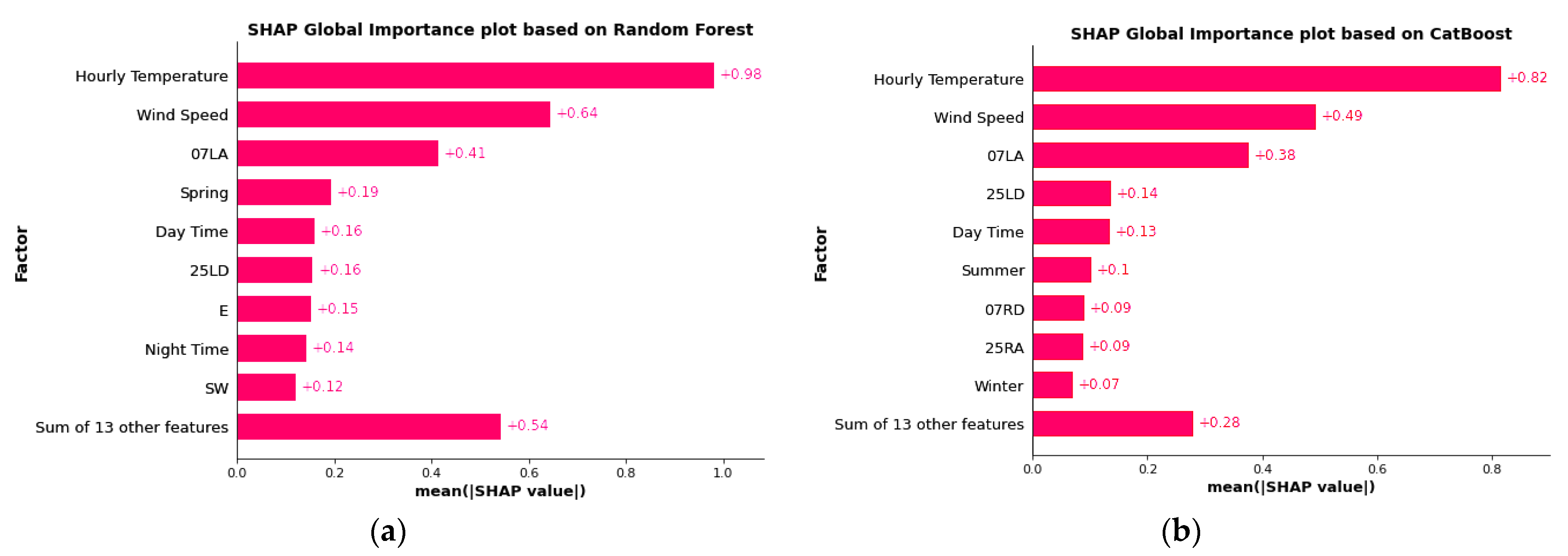
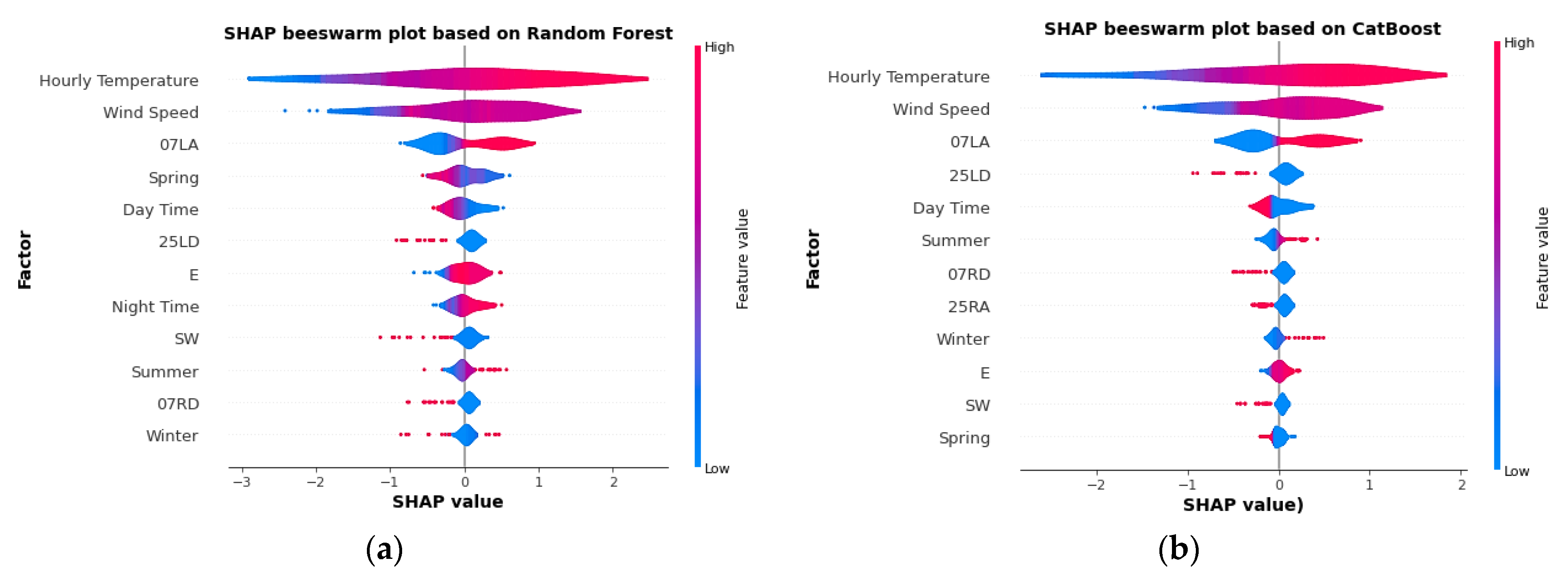
3.3.1. Global Factors’ Importance and Contribution

For the global factors’ importance and contribution analysis, we used the BO-Random Forest classifier, which was the best model in our case, followed by the BO-CatBoost classifier, which was the second-best model. In using these two optimal models with accurate LLWS criticality predictions, there was strong merit in investigating which factors were the most important and quantifying how these factors contributed to the final predictions. To explore the impact of each factor on the final prediction, the SHAP values were used. It is worth mentioning that factor importance is not the same as factor contribution. Factor importance indicates which factors have the greatest impact on a model’s performance. The factor contributions not only identify relevant factors, but they also provide a logical explanation for the observed outcome (NC-LLWS or C-LLWS). This study determined the importance of each factor and its contribution to the model estimate using the top two BO-ELCs with better accuracies. Figure 10a illustrates the SHAP global importance scores for the factors used in the BO-Random Forest classifier. However, the outcome did not indicate the proportionate contribution of each factor to the likelihood of an LLWS criticality. It showed that the most important factor that caused the occurrence of C-LLWS was the hourly temperature, which had a mean SHAP value of +0.98, followed by the mean wind speed with a mean SHAP value of +0.64 and Runway 07LA (+0.41). Figure 10b illustrates the SHAP global importance scores for the factors using the CatBoost model. The results revealed that the most important factor that caused C-LLWS was the hourly temperature (+0.82) followed by wind speed (+0.49) and Runway 07LA (+0.38). The sequences of the factor importance in the case of both the BO-Random Forest classifier and the BO-CatBoost classifier were consistent, while there was a slight difference in their SHAP values.
Similarly, a SHAP contribution evaluation was conducted to conduct a more in-depth examination of the Random Forest and CatBoost models using SHAP beeswarm plots (Figure 11). We created a quantitative value from the SHAP contribution plots that combined the Shaply values and expressed the classifier contributions of factors. The input factors were arranged on the vertical axis in order of increasing influence, starting with the most influential. The SHAP value is shown on the horizontal axis, and the significance of the factor is shown by the color scale, (blue to pinkish-red for low significance to high significance). The SHAP beeswarm plots of the Random Forest and CatBoost models illustrate that most of the moderate-to-high mean wind speeds resulted in the occurrence of C-LLWS events, which are represented by the pinkish-red color toward the right side of the vertical reference line with positive SHAP values (Figure 11a,b). The blue color toward the left of the vertical reference line indicates the occurrence of NC-LLWS events due to a low mean wind speed. Similarly, in the case of the mean hourly temperature, a high temperature (represented in red) is shown to the right of the vertical reference line with a positive SHAP value and blue to the left of the vertical reference line. It shows that high temperatures resulted in C-LLWS events while low temperatures were more likely to cause NC-LLWS events. The same was the case for wind speed and Runway 07LA.

3.3.2. Factor Dependence and Interaction

There was no obvious correlation between the changes in the factor value and the changes in the SHAP value in the factor global importance and contribution (beeswarm) plot. Figure 12 supplements the contribution plot by providing more information about how the SHAP values varied with the eigenvalues and by displaying the individual interpretation outcomes for the three major factors. The SHAP dependence and interaction plots were examined to ascertain the extent to which the input variables used to evaluate the Random Forest classifier interacted in terms of their contributions (see Figure 12). The SHAP dependence plot is a scatter plot that demonstrates the effect a single factor had on the predictions made by the classifier, which in our case was the Random Forest model. The SHAP interaction plot shows the effect of two factors on the models’ predictions.
The dependence and interaction plot examines the top three influential factors; namely, hourly temperature, wind speed, and Runway 07LA. Other factor interactions, however, could be explored as well. Figure 12a depicts the effect of wind speed on the models’ predictions. The points with high density fell above the SHAP 0.0 reference line and at wind speeds of more than 4.4 m/s up to 8 m/s had a positive impact on the prediction of LLWS, which meant that wind speeds higher than 4.4 m/s were more likely to cause C-LLWS events. The results were consistent with the findings of previous studies [41,42]. However, it is pertinent to mention that for the occurrence of C-LLWS events, the variation in wind speed is more important than the mean wind speed. The duration of a C-LLWS event that might be encountered by an aircraft is generally within a few seconds to a few minutes. Therefore, the hourly mean wind speed can hardly provide an accurate indication of LLWS criticality. Therefore, more refined data on wind conditions such as a 1 min mean in turbulence intensity may be required to improve the models’ accuracies.
Figure 12b depicts the effect of hourly temperature on the models’ predictions. The points with high density fell above the SHAP 0.0 reference line at an hourly temperature of 23 °C to 31 °C, which had a positive impact on the predictions of LLWS. This illustrated that C-LLWS events were more likely to occur at temperatures between 23 °C and 31 °C. The SHAP value for Runway 07LA when labeled ‘1’ was higher than reference 0.0 and lower when labeled as ‘0′ (Figure 12c). This illustrated that Runway 07LA was highly vulnerable to the occurrence of C-LLWS events. This also showed that C-LLWS events were more likely to occur under the easterly, southeasterly, southerly, and southwesterly winds, which was also consistent with the previous findings [5,43,44]. Pilots should be cautious when making a “final approach” to Runway 07LA. Figure 12d demonstrates the interaction of the wind speed and hourly temperature and their combined influence on the BO-Random Forest classifier prediction. When the wind speed ranged from 4.2 m/s to 9.8 m/s and the hourly temperature ranged from 24.8 °C to 29.5 °C, high density points formed in the shaded area above the SHAP 0.0 reference line. Within these ranges, C-LLWS events were more likely to occur.

3.3.3. Local Factor Interpretation

Figure 13 shows the SHAP explanatory force chart for two randomly selected cases from the actual estimations. The base value (0.045) on the graph represents the mean of the BO-Random Forest classifier estimations for the training data set. The NC-LLWS condition occurred when the outcome value of classifier was less than the classifier’s base value. C-LLWS events occurred when the classifier’s output value exceeded the base value. The blue arrows illustrate the magnitude of an input factor’s effect on the likelihood of an NC-LLWS occurrence. The likelihood of occurrence of a C-LLWS event was influenced by input factors as indicated by the red arrows. Each arrow’s area occupied by a factor reflects the magnitude of that factor’s effect. Consider two instances of the BO-Random Forest classifier that were correctly classified as C-LLWS and NC-LLWS from the training dataset. The two instances depicted in Figure 13 correctly classified as NC-LLWS and C-LLWS had estimated values of −2.91 and 3.62, respectively. For the first randomly selected instance (Figure 13a), when the wind speed was equal to 3.4 m/s with a moderate hourly temperature equal to 23.8 °C, an NC-LLWS occurred. This figure also illustrates that seasons other than spring can have occurrences of NC-LLWS events. The spring season designated as 0 highlighted that for this randomly selected instance, the spring season did not contribute to the occurrence of NC-LLWS events. Contrary to this (Figure 13b), the combination of a moderate temperature equal to 21.6 °C with a high wind speed and spring season, a C-LLWS event occurred. However, the autumn season did not contribute to the occurrence of C-LLWS events. Similarly, for this very instance, Runway 07LA contributed to the occurrence of a C-LLWS event. In a similar fashion, we could randomly select other correctly classified instances for their local interpretation.

4. Conclusions and Recommendations

This study presented the application of five state-of-the-art BO-ELCs in the prediction of the occurrence of an LLWS criticality. Six factors, including the hourly temperature, wind speed, runway orientation, wind direction, time of day, season, and the height of the LLWS as a binary target factor from the PIREPs and HKO weather reports, were used as inputs. Under the comprehensive evaluation criteria, all models achieved a high prediction accuracy. Nevertheless, ensemble learning algorithms are frequently criticized for their lack of interpretability and transparency. Despite the fact that engineering-domain models are more flexible and frequently more accurate than traditional predictive statistical techniques, this has an effect on their widespread acceptability. In this study, the model with the best prediction was interpreted using the SHAP algorithm, and the influence of the top three factors on the occurrence of an LLWS criticality was demonstrated. Based on the study, the following conclusions were drawn:
  • In the testing dataset, the BO-Random Forest classifier had the best overall performance of all BO-ELCs investigated in this study with an AUC-ROC of 0.759 and accuracy, precision, recall, F1-score, and AUC-PRC values of 0.714, 0.724, 0.710, 0.713, and 0.75, respectively.
  • The performance of each individual BO-ELC varied marginally. Despite the fact that XGBoost’s AUC-ROC was 0.73, its accuracy, recall, precision, F1-score, and AUC-PRC values were 0.652, 0.656, 0.664, 0.656, and 0.68, respectively.
  • The AdaBoost and LGBM models demonstrated the lowest AUC-ROC (0.687) and AUC-PRC (0.67) scores, respectively.
  • SHAP demonstrated efficacy in interpreting the optimal model’s outcome (BO-Random Forest classifier). In terms of the factor influence, the SHAP analysis revealed that the hourly temperature is the most influential factor followed by the wind speed and runway 07LA.
  • When the wind speed was moderate to high (>4.2 m/s) and the temperature was moderate to high (>24.5 °C), aircrafts on a final approach to Runway 07LA were more likely to experience critical LLWS.
The technique proposed in this research work can be utilized to undertake a large-scale investigation of wind shear and can serve as a useful resource for aviation authorities and researchers who are concerned with aviation safety. In addition, this paper focused exclusively on the prediction of LLWS criticality as computed by using five BO-ELC classifiers (CatBoost, XGBoost, LGBM, RF, and AdaBoost) in aggregation with the SHAP model. This study was limited to the application of machine learning models. Future studies might be undertaken by combining a number of other BO-ELCs such as a stacking ensemble as well as neural network models with a range of additional risk factors such as inter-annual changes in wind shear events and their spatial distributions.

Author Contributions

Conceptualization, A.K. and P.-W.C.; Data curation, P.-W.C.; Formal analysis, A.K.; Funding acquisition, P.-W.C. and F.C.; Investigation, A.K., F.C., and H.P.; Methodology, A.K.; Project administration, F.C.; Resources, H.P.; Validation, F.C.; Writing—original draft, A.K.; Writing—review and editing, H.P. All authors have read and agreed to the published version of the manuscript.

Funding

This research was supported by the National Natural Science Foundation of China (U1733113), the Shanghai Municipal Science and Technology Major Project (2021SHZDZX0100), the Research Fund for International Young Scientists (RFIS) of the National Natural Science Foundation of China (NSFC) (Grant No. 52250410351), and the National Foreign Expert Project (Grant No. QN2022133001L).

Institutional Review Board Statement

Not applicable.

Informed Consent Statement

Not applicable.

Data Availability Statement

Not applicable.

Acknowledgments

We are thankful to the Hong Kong Observatory at Hong Kong International Airport for providing us with the pilot reports and weather-related data.

Conflicts of Interest

The authors declare no conflict of interest.

References

  1. ACI. Annual World Airport Traffic Report; ACI: Montreal, QC, Canada, 2018. [Google Scholar]
  2. Fichtl, G.H.; Camp, D.W.; Frost, W. Sources of low-level wind shear around airports. J. Aircr. 1977, 14, 5–14. [Google Scholar] [CrossRef]
  3. Bretschneider, L.; Hankers, R.; Schönhals, S.; Heimann, J.M.; Lampert, A. Wind Shear of Low-Level Jets and Their Influence on Manned and Unmanned Fixed-Wing Aircraft during Landing Approach. Atmosphere 2021, 13, 35. [Google Scholar] [CrossRef]
  4. Michelson, M.; Shrader, W.; Wieler, J. Terminal Doppler weather radar. Microw. J. 1990, 33, 139. [Google Scholar]
  5. Shun, C.; Chan, P. Applications of an infrared Doppler LiDAR in detection of wind shear. J. Atmos. Ocean. Technol. 2008, 25, 637–655. [Google Scholar] [CrossRef]
  6. Li, L.; Shao, A.; Zhang, K.; Ding, N.; Chan, P.-W. Low-level wind shear characteristics and LiDAR-based alerting at Lanzhou Zhongchuan International Airport, China. J. Meteorol. Res. 2020, 34, 633–645. [Google Scholar] [CrossRef]
  7. Thobois, L.; Cariou, J.P.; Gultepe, I. Review of LiDAR-based applications for aviation weather. Pure Appl. Geophys. 2019, 176, 1959–1976. [Google Scholar] [CrossRef]
  8. Hon, K.-K. Predicting low-level wind shear using 200-m-resolution NWP at the Hong Kong International Airport. J. Appl. Meteorol. Climatol. 2020, 59, 193–206. [Google Scholar] [CrossRef]
  9. Chan, P. A tail strike event of an aircraft due to terrain-induced wind shear at the Hong Kong International Airport. Meteorol. Appl. 2014, 21, 504–511. [Google Scholar] [CrossRef]
  10. Lei, L.; Chan, P.; Li-Jie, Z.; Hui, M. Numerical simulation of terrain-induced vortex/wave shedding at the Ho;ng Kong International Airport. Meteorol. Z. 2013, 22, 317–327. [Google Scholar] [CrossRef]
  11. Chan, P.; Hon, K. Observation and numerical simulation of terrain-induced wind shear at the Hong Kong International Airport in a planetary boundary layer without temperature inversions. Adv. Meteorol. 2016, 2016, 1454513. [Google Scholar] [CrossRef]
  12. Shimoyama, K.; Nakanomyo, H.; Obayashi, S. Airport terrain-induced turbulence simulations integrated with weather prediction data. Trans. Jpn. Soc. Aeronaut. Space Sci. 2013, 56, 286–292. [Google Scholar] [CrossRef]
  13. Casado-Sanz, N.; Guirao, B.; Lara Galera, A.; Attard, M. Investigating the risk factors associated with the severity of the pedestrians injured on Spanish crosstown roads. Sustainability 2019, 11, 5194. [Google Scholar] [CrossRef] [Green Version]
  14. Shaik, M.E.; Islam, M.M.; Hossain, Q.S. A review on neural network techniques for the prediction of road traffic accident severity. Asian Transp. Stud. 2021, 7, 100040. [Google Scholar] [CrossRef]
  15. Mujalli, R.O.; de Oña, J. Injury severity models for motor vehicle accidents: A review. In Proceedings of the Institution of Civil Engineers-Transport; Thomas Telford Ltd.: London, UK, 2013; pp. 255–270. [Google Scholar]
  16. Yuan, C.; Li, Y.; Huang, H.; Wang, S.; Sun, Z.; Li, Y. Using traffic flow characteristics to predict real-time conflict risk: A novel method for trajectory data analysis. Anal. Methods Accid. Res. 2022, 35, 100217. [Google Scholar] [CrossRef]
  17. Zhao, Y.; Deng, W. Prediction in Traffic Accident Duration Based on Heterogeneous Ensemble Learning. Appl. Artif. Intell. 2022, 1–24. [Google Scholar] [CrossRef]
  18. Zhang, S.; Khattak, A.; Matara, C.M.; Hussain, A.; Farooq, A. Hybrid feature selection-based machine learning Classification system for the prediction of injury severity in single and multiple-vehicle accidents. PLoS ONE 2022, 17, e0262941. [Google Scholar] [CrossRef]
  19. Goodman, S.N.; Goel, S.; Cullen, M.R. Machine learning, health disparities, and causal reasoning. Ann. Intern. Med. 2018, 169, 883–884. [Google Scholar] [CrossRef]
  20. Guo, R.; Fu, D.; Sollazzo, G. An ensemble learning model for asphalt pavement performance prediction based on gradient boosting decision tree. Int. J. Pavement Eng. 2022, 23, 3633–3646. [Google Scholar] [CrossRef]
  21. Liu, J.N.; Kwong, K.; Chan, P.W. Chaotic oscillatory-based neural network for wind shear and turbulence forecast with LiDAR data. IEEE Trans. Syst. Man Cybern. Part C 2012, 42, 1412–1423. [Google Scholar] [CrossRef]
  22. Guidotti, R.; Monreale, A.; Ruggieri, S.; Pedreschi, D.; Turini, F.; Giannotti, F. Local rule-based explanations of black box decision systems. arXiv 2018, arXiv:1805.10820. [Google Scholar]
  23. Rudin, C. Stop explaining black box machine learning models for high stakes decisions and use interpretable models instead. Nat. Mach. Intell. 2019, 1, 206–215. [Google Scholar] [CrossRef] [PubMed] [Green Version]
  24. Lundberg, S.M.; Lee, S.-I. A unified approach to interpreting model predictions. Adv. Neural Inf. Process. Syst. 2017, 30. [Google Scholar]
  25. Merrick, L.; Taly, A. The explanation game: Explaining machine learning models using Shapley values. In Proceedings of the International Cross-Domain Conference for Machine Learning and Knowledge Extraction, Dublin, Ireland, 25–28 August 2020; pp. 17–38. [Google Scholar]
  26. Dong, S.; Khattak, A.; Ullah, I.; Zhou, J.; Hussain, A. Predicting and analyzing road traffic injury severity using boosting-based ensemble learning models with SHAPley Additive exPlanations. Int. J. Environ. Res. Public Health 2022, 19, 2925. [Google Scholar] [CrossRef] [PubMed]
  27. Mangalathu, S.; Hwang, S.H.; Jeon, J.S. Failure mode and effects analysis of RC members based on machine-learning-based SHapley Additive exPlanations (SHAP) approach. Eng. Struct. 2020, 219, 110927. [Google Scholar] [CrossRef]
  28. Khattak, A.; Almujibah, H.; Elamary, A.; Matara, C.M. Interpretable Dynamic Ensemble Selection Approach for the Prediction of Road Traffic Injury Severity: A Case Study of Pakistan’s National Highway N-5. Sustainability 2022, 14, 12340. [Google Scholar] [CrossRef]
  29. Feng, D.C.; Wang, W.J.; Mangalathu, S.; Taciroglu, E. Interpretable XGBoost-SHAP machine-learning model for shear strength prediction of squat RC walls. J. Struct. Eng. 2021, 147, 04021173. [Google Scholar] [CrossRef]
  30. García, M.V.; Aznarte, J.L. Shapley additive explanations for NO2 forecasting. Ecol. Inform. 2020, 56, 101039. [Google Scholar] [CrossRef]
  31. Wu, J.; Chen, X.Y.; Zhang, H.; Ziong, I.-D.; Lei, H.; Deng, S.-H. Hyperparameter optimization for machine learning models based on Bayesian optimization. J. Electron. Sci. Technol. 2019, 17, 26–40. [Google Scholar]
  32. Shekar, B.; Dagnew, G. Grid search-based hyperparameter tuning and classification of microarray cancer data. In Proceedings of the 2019 2nd International conference on advanced computational and communication paradigms (ICACCP), Sikkim, India, 25–28 February 2019; pp. 1–8. [Google Scholar]
  33. Kadam, V.J.; Jadhav, S.M. Performance analysis of hyperparameter optimization methods for machine learning with small and medium sized medical datasets. J. Discret. Math. Sci. Cryptogr. 2020, 23, 115–123. [Google Scholar] [CrossRef]
  34. Ke, G.; Meng, Q.; Finley, T.; Wang, T.; Chen, W.; Ma, W.; Ye, Q.; Liu, T.Y. LightGBM: A highly efficient gradient boosting decision tree. Adv. Neural Inf. Process. Syst. 2017, 30. [Google Scholar]
  35. Parmar, A.; Katariya, R.; Patel, V. A review on random forest: An ensemble classifier. In Proceedings of the International Conference on Intelligent Data Communication Technologies and Internet of Things, Coimbatore, India, 7–8 August 2018; pp. 758–763. [Google Scholar]
  36. Chen, T.; Guestrin, C. Xgboost: A scalable tree boosting system. In Proceedings of the 22nd ACM SIGKDD International Conference on Knowledge Discovery and Data Mining, San Francisco, CA, USA, 13–17 August 2016; pp. 785–794. [Google Scholar]
  37. Hancock, J.T.; Khoshgoftaar, T.M. CatBoost for big data: An interdisciplinary review. J. BIG Data 2020, 7, 1–45. [Google Scholar] [CrossRef] [PubMed]
  38. An, T.-K.; Kim, M.-H. A new diverse AdaBoost classifier. In Proceedings of the 2010 International conference on artificial intelligence and computational intelligence, Sanya, China, 23–24 October 2010; pp. 359–363. [Google Scholar]
  39. Chan, P.W. A significant wind shear event leading to aircraft diversion at the Hong Kong international airport. Meteorol. Appl. 2012, 19, 10–16. [Google Scholar] [CrossRef]
  40. Chan, P. Severe wind shear at Hong Kong International airport: Climatology and case studies. Meteorol. Appl. 2017, 24, 397–403. [Google Scholar] [CrossRef] [Green Version]
  41. Chen, F.; Peng, H.; Chan, P.W.; Ma, X.; Zeng, X. Assessing the risk of wind shear occurrence at HKIA using rare-event logistic regression. Meteorol. Appl. 2020, 27, e1962. [Google Scholar] [CrossRef]
  42. Chan, P.W.; Hon, K.K. Observations and numerical simulations of sea breezes at Hong Kong International Airport. Weather 2022. [CrossRef]
  43. Chen, F.; Peng, H.; Chan, P.-w.; Zeng, X. Low-level wind effects on the glide paths of the North Runway of HKIA: A wind tunnel study. Build. Environ. 2019, 164, 106337. [Google Scholar] [CrossRef]
  44. Chen, F.; Peng, H.; Chan, P.-w.; Zeng, X. Wind tunnel testing of the effect of terrain on the wind characteristics of airport glide paths. J. Wind. Eng. Ind. Aerodyn. 2020, 203, 104253. [Google Scholar] [CrossRef]
Figure 1. Occurrence location of LLWS events in the vicinity of an airport runway.
Atmosphere 13 02102 g001
Figure 2. Detrimental and potentially hazardous effects of LLWS on approaching aircraft: (a) declining headwind during final approach; (b) rising headwind during final approach.
Atmosphere 13 02102 g002
Figure 3. Framework for the prediction and interpretation of LLWS criticality at the vicinity of runways at HKIA.
Atmosphere 13 02102 g003
Figure 4. Hong Kong International Airport and surrounding terrain.
Atmosphere 13 02102 g004
Figure 5. Hybrid BO-ELC approach for the prediction of LLWS criticality.
Atmosphere 13 02102 g005
Figure 6. Confusion matrix plot.
Atmosphere 13 02102 g006
Figure 7. (a) LLWS events with respect to runway; (b) LLWS events with respect to wind direction; (c) LLWS events with respect to day/night; (d) LLWS events with respect to season of year; (e) box plot of hourly temperature; (f) box plot of wind speed.
Atmosphere 13 02102 g007aAtmosphere 13 02102 g007b
Figure 8. Combined ROC curve for all Bayesian-optimized ELC models.
Atmosphere 13 02102 g008
Figure 9. Combined precision–recall curve (PRC) for all Bayesian-optimized ELC models.
Atmosphere 13 02102 g009
Figure 10. SHAP global importance plots: (a) Random Forest; (b) CatBoost.
Atmosphere 13 02102 g010
Figure 11. SHAP beeswarm plots: (a) Random Forest; (b) CatBoost.
Atmosphere 13 02102 g011
Figure 12. (a) SHAP wind speed dependence plot; (b) SHAP hourly temperature dependence plot output; (c) SHAP Runway 07LA dependence plot; (d) SHAP interaction plot of wind speed and hourly temperature.
Atmosphere 13 02102 g012
Figure 13. SHAP explanatory force plots: (a) plot of case with a value equal to 0.291; (b) plot of case with a value equal to 3.62.
Atmosphere 13 02102 g013
Table 1. One-hot encoding of categorical factors for the modeling.
FactorCodes and Description
Runway Orientation
07LA1: If a wind shear event is reported at Runway 07LA, 0: Otherwise
07RA1: If a wind shear event is reported at Runway 07RA, 0: Otherwise
25RA1: If a wind shear event is reported at Runway 25RA, 0: Otherwise
25LA1: If a wind shear event is reported at Runway 25LA, 0: Otherwise
25LD1: If a wind shear event is reported at Runway 25LD, 0: Otherwise
07RD1: If a wind shear event is reported at Runway 07LD, 0: Otherwise
Wind Direction
N1: If wind direction is North, 0: Otherwise
NE1: If wind direction is North-East, 0: Otherwise
E1: If wind direction is East 0: Otherwise
SE1: If wind direction is South-East, 0: Otherwise
S1: If wind direction is South, 0: Otherwise
SW1: If wind direction is South-West, 0: Otherwise
W1: If wind direction is West, 0: Otherwise
NW1: If wind direction is North-West, 0: Otherwise
Season of the Year
Winter1: If a wind shear event occurs in Winter, 0: Otherwise
Spring1: If a wind shear event occurs in Spring, 0: Otherwise
Summer1: If a wind shear event occurs in Summer, 0: Otherwise
Autumn1: If a wind shear event occurs in Autumn, 0: Otherwise
Time of the Day
Day Time1:If a wind shear event occurs during day time, 0: Otherwise
Night Time1:If a wind shear event occurs during night time, 0: Otherwise
Table 2. Hyperparameter tunings of ELCs.
AlgorithmHyperparametersRangeOptimal Values
LGBM{(n_estimators), (num_leaves), (learning rate), (reg_lambda), (reg_alpha}{(100–1500), (30–100), (0.001–0.2), (1.1–1.5), (1.1–1.5)}{900, 38, 0.07, 1.24, 1.18}
CatBoost{(n_estimators), (max_depth), (learning rate)}{(200–1500), (2–15), (0.001–0.2)}{727, 5, 0.1}
AdaBoost{(n_estimators), (learning rate)}{(100–1500), (0.001–0.2)}{871, 0.08}
RF{(n_estimators), (max_depth)}{(50–1000), (2–15)}{1041, 7}
XGBoost{(n_estimators), (num_leaves), (learning rate), (reg_lambda), (reg_alpha}{(100–1500), (30–100), (0.001–0.2), (1.1–1.5), (1.1–1.5)}{1105, 46, 0.05, 1.41, 1.27}
Table 3. Performance measures of BO-ELCs.
BO-ELCPerformance Metrics
AccuracyPrecisionRecallF1-Score
LGBM0.6720.6810.6720.676
AdaBoost0.6810.6730.6610.663
Random Forest0.7140.7240.7100.713
CatBoost0.6810.6740.6890.686
XGBoost0.6520.6640.6520.656
Publisher’s Note: MDPI stays neutral with regard to jurisdictional claims in published maps and institutional affiliations.

