
How Much Photovoltaic Efficiency Is Enough?

Institute for Photovoltaics and Research Center SCoPE, Pfaffenwaldring 47, 70569 Stuttgart, Germany
Solar 2022, 2(2), 215-233; https://doi.org/10.3390/solar2020012
Submission received: 26 February 2022
/
Revised: 7 April 2022
/
Accepted: 12 April 2022
/
Published: 14 April 2022
(This article belongs to the Special Issue Solar Technologies—A Snapshot of the Editorial Board)
Abstract
:At present, the purchasing prices for silicon-based photovoltaic modules with 20% efficiency and more are between 20 and 40 EURct/Wp. These numbers correspond to 40 to 80 EUR/m2 and are in the same range as the mounting costs (material prices plus salaries) of such modules. Installers and operators of photovoltaic systems carefully balance the module and mounting costs when deciding among modules of different efficiencies. This contribution emulates the installer’s decision via a simple, analytical module mounting decision (Mo2De) model. A priori, the model, and the resulting conclusions are completely independent of the photovoltaically active material inside the modules. De facto, however, based on the present state (cost, efficiency, reliability, bankability, etc.) of modules fabricated from (single) crystalline Si cells, conclusions on other photovoltaic materials might also be drawn: On the one hand, the model suggests that lower-efficiency modules with efficiencies below 20% will be driven out of the market. Keeping in mind their installation costs, installers will ask for large discounts for lower-efficiency modules. Technologies based on organic semiconductors, CdTe, CIGS, and even multicrystalline Si, might not survive in the utility market, or in industrial and residential applications. Moreover, this 20% mark will soon reach 23%, and finally will stop at around 25% for the very best, large-area (square meter sized) commercial modules based on single crystalline silicon only. On the other hand, it also seems difficult for future higher-efficiency modules based on tandem/triple cells to compete with standard Si-based reference modules. Compared to their expected higher efficiency, the production costs of tandem/triple cell modules and, therefore, also their required markup in sales, might be too high. Depending on the mounting cost, the Mo2De-model predicts acceptable markup values of 1 EURct/Wp (for low mounting costs of around 10 EUR/m2) to 11 EURct/Wp (for high mounting costs of 100 EUR/m2) if the module efficiency increases from 23% to 30%. Therefore, a 23% to 24% module efficiency, which is possible with silicon cells alone, might be enough for many terrestrial photovoltaic applications.
1. Introduction
Almost seventy years ago, photovoltaics (PV) started as a byproduct of microelectronics [1]. At the end of the year 2020, more than 700 GWp of photovoltaic power was installed world-wide [2]. In 2021, an additional 150 GWp was added [3]. With over 200 GWp in annual module production capacity, this year, the photovoltaic power installed world-wide will surpass the 1 TWp-mark. Therefore, the prefix “tera” instead of “micro” is characteristic for today’s photovoltaic technology. The technology of wafer-based crystalline silicon solar cells has led us into the Terra-electronics age. [Terra (Latin) = Earth].
In the annual PV market, modules based on crystalline silicon make up 95% of all sales [2]. Within the last ten years, amorphous/microcrystalline silicon disappeared from the market completely, and other thin-film materials such as CdTe and Cu(In,Ga)Se2 steadily lost market shares [2]. The market share of other materials is practically zero. This finding completely adheres to an earlier publication [4] of the present author, which, already in 2004, questioned the success of “second generation photovoltaics”, i.e., of thin-film-based modules. These doubts were based on the author’s own research, performed over ten years, on thin-film cells composed of crystalline silicon and Cu(In,Ga)Se2 [5,6]. Indeed, thin film PV modules did not take over the market, despite the steady exponential growth of the total market since then. Additionally, the hype around so-called “third generation” photovoltaics [7,8] quietly disappeared in the meantime. It will be interesting to see if the present hype around perovskite-type cells, triggered by the sensational results of research on them [9,10], will do the same. Will it really lead to industrially mass-produced, low-cost, long-lasting modules? Furthermore, beyond second and third generation concepts, today, fourth generation photovoltaics are also being discussed in the scientific community [11].
Despite all these scientifically interesting ideas, the photovoltaic revolution, and the real state of photovoltaics outside of research labs is being governed, driven, and even accelerated by cells made from wafered crystalline silicon. The market share of second-generation photovoltaics has dropped to 5% [2], and most third generation concepts [7,8] (including my own [12]) did not even make it from the design stage to become real cells in the lab. Fourth generation materials [11] are also far from industrial cells.
Large-area silicon-cell-based modules with efficiencies around 20% are standard today. Soon, these modules will reach approximately 23 to 24% efficiency. This overall increase in module efficiency is being driven by research on high-efficiency silicon cells and the success in fabricating those cells with large areas (around and above 250 cm2) in huge, high-throughput factories up to efficiencies around 23% for below 20 EURct/Wp. The best industrial cells can currently reach up to 25% efficiency [13], and the world record for lab-based cells is at 26.7% [14].
Within the next few years, the increase in efficiency of silicon solar cells will come to an end: the upper theoretical limit is 29% [15]. It seems possible that even under the conditions of industrial mass production, large area cells with approximately 26% efficiency will be fabricated. However, it will be hard to do this at a low cost.
When the cells are packed into solar modules, the efficiency almost unavoidably drops by 1 to 2% absolute, as the result of optical reflection on the front glass and via electrical mismatch losses among slightly different, series-connected cells. Additionally, there are small gaps between neighboring module strings and often also between neighboring, series-connected cells. In addition, there must be a small distance between the outermost cells and the edges of the frame or the edges of the glass plate. This gap increases the isolation resistance of the modules and minimizes the potential induced degradation (PID) of the cells, particularly in systems that operate at DC-voltages up to 1500 V [16]. Consequently, the module area is larger than the total cell area, leading to a drop in the module’s efficiency when compared to the cells’ efficiency. Therefore, I estimate an upper practical limit of solar module efficiency around 25% solar efficiency in the very best, large area, silicon-based industrial modules of the future. Thus, from the present case of around 20% module efficiency, there is still 5% to be gained by those very best (most expensive) pure Si-based modules. Future “reasonable priced” modules for the large-area, and low-cost production of photovoltaic electricity will probably reach around 23 to 24% efficiency.
Is an efficiency of 23% in photovoltaic modules enough? In other words, is it economically viable to increase the efficiency further, for example by producing solar modules that contain Si/perovskite tandem cells or even by completely replacing the semiconductor silicon in photovoltaic modules?
This contribution takes the standpoint of an installer who must decide between photovoltaic modules of different efficiencies. The decision is emulated by a simple, analytical module mounting decision (Mo2De) model, which emphasizes the importance of mounting cost. Seen from the installer’s perspective, (future) purely silicon-based photovoltaic modules with 23% to 24% efficiency (or even lower) might represent the best and most economic choice for most (terrestrial) photovoltaic applications.
Therefore, it might be hard for the producers/distributors of future high-efficiency modules based on tandem cells made of Si/perovskites (or any other material combination) to compete with the 23% efficient, “standard” modules made from Si only. For installers, all higher efficiency modules are interesting, because they entail that fewer modules, less mounting material, and less time are needed to erect a photovoltaic system of fixed power. Thus, in principle, installers are willing to pay a markup/surcharge for higher-efficiency modules when compared to “standard” modules. However, this markup depends on mounting costs and is limited. The surcharge might not be sufficient for module producers to compensate for the additional production costs, which are necessary if tandem cell modules are to exceed the efficiency limits of “normal” high-efficiency, purely silicon-based modules. Nevertheless, future modules with efficiencies above the efficiency limits of silicon might be interesting in cases of unusually high mounting costs and for systems with very limited space.
2. The Photovoltaic Brick Stone
Table 1 compares the present areal prices of standard silicon-based modules with an efficiency of 20% to other construction materials. The square meter prices of the construction materials are typical wholesale prices paid by craftsmen and also seen in hardware stores in Germany.
The assumed range of power-related module prices from M€ = 20 EURct/Wp = 200 EUR/kWp to M€ = 40 EURct/Wp = 400 EUR/kWp for the η = 20% efficient module under consideration corresponds to area related module prices from M□ = 40 EUR/m2 to M□ = 80 EUR/m2. These prices are realistic for the year 2022. Based on the own author’s experiences, these prices are even lower sometimes, and over time they will drop even more.
According to Table 1, the square meter price for Si-based photovoltaic modules falls in the same range as those of other construction materials used for buildings: steel, glass, windows, brick stones, etc. Therefore, considering not only the modularity but also the area-related cost, it is instructive and fair to look at PV modules as “electric brick stones” used for electricity supply. Small PV systems need only a few brick stones, while larger ones need more.
To produce 1 kWp of electric power with 20% efficient modules (measured under standard testing conditions) requires an area of 5 m2. Modules with η = 10% (e.g., from organic cells) would require 10 m2, the η = 5% modules (e.g., from amorphous Si with one pin-junction) would require 20 m2. Could such low-efficiency modules ever be competitive?
If, for the moment, we neglect the increasing areal mounting cost, MOUNT□ (which is discussed later), such low efficiency modules would have to be sold for M□ = 20 EUR/m2 (in the case of η = 10%) and M□ = 10 EUR/m2 (in the case of η = 5% efficiency), in order to compete with the η = 20% efficient modules at a purchasing price of 20 EURct/Wp (40 EUR/m2). Clearly, such prices are close to, and can even be below, the production and material costs of the lower-efficiency modules—especially, when two glass plates are needed. Unfortunately, most thin film modules do need two glass plates, in order to protect either the photovoltaic material itself, or the conductive ZnO or InOx, against air humidity. It is therefore understandable, that, for example, amorphous and microcrystalline silicon has almost completely disappeared from the module market. Below, this will be discussed in more detail. The competition between photovoltaic materials was/is not limited only to “crystalline silicon against other PV materials”. There is also a competition between different Si technologies: Modules from amorphous and microcrystalline Si have not survived, and even the large area tandem/triple cell modules fought to reach the 10% efficiency mark. Also, some silicon technologies using defective multicrystalline silicon did not reach 15 to 16% efficiency; as a consequence, they completely disappeared from the market: Cells made via the edge defined film fed growth (EFG) technique [17] of SCHOTT Solar GmbH, the string ribbon (SR) technology of Evergreen Solar Inc., and SOVELLO GmbH [18,19], and the ribbon growth on substrate (RGS) approach of SolarWorld AG [20], were the last examples ribbon-based silicon technologies. In addition, within the last few years, even block cast multicrystalline silicon has lost more and more market shares [1]. The efficiencies of multicrystalline cells are too low when compared to those made of single crystalline wafers.
In the past, the research on, and the market of multicrystalline Si cells, was based on the high price of single crystalline Si wafers. However, this is no longer the case. Today, the typical prices for n-type, high minority carrier lifetime, single crystalline Si wafers are around 15 to 30 EUR/m2 [21]. Using such wafers, it is possible to produce cells up to 25% efficiency via industrial mass production. As a consequence, multicrystalline Si technologies are disappearing.
Again, a comparison with Table 1: With a 15 to 30 EUR/m2 purchasing price even for small quantities (1000 wafers), single crystalline Si wafers often are cheaper than ceramic tiles. In fact, sometimes it seems cheaper to use single crystalline Si wafers instead of ceramic tiles to tile bathrooms. Just to remember, from all the materials that mankind has ever made, the single crystalline Si wafer is the most regular, perfect, and clean. This is important when considering other “low-cost” photovoltaic materials or “solar paints”. In addition to being cheap, crystalline silicon has other advantages: it is non-toxic, stable in all aspects, bendable when thin enough; its elastic properties are close to those of steel. Thus, at the present stage of the photovoltaic revolution, it will be very hard—if not impossible—to ever beat or replace crystalline silicon as a photovoltaic material in almost any terrestrial photovoltaic application. This will be discussed further below.
The data in Table 1 show the prices for the PV materials/modules themselves. The balance of the systems and the costs (materials plus salaries) of mounting the photovoltaic modules have not been considered yet. The following discussions show, on the one hand, that the financial situation for the lower-efficiency modules is even worse than that described in Table 1. On the other hand, it is better for the higher-efficiency modules. Those with twice the efficiency of standard modules could be sold for more than twice the price, and installers would pay more because they also consider savings on the mounting costs.
3. Total Cost T of an Installed Photovoltaic System
3.1. Balance of System BOS: Mounting Cost MOUNT and Fixed Cost FIX
Here, we adopt the viewpoint of a PV installer (or owner/operator) who has to purchase modules and installs (and eventually also operate) the complete PV system. Installers regularly have to make economic decisions between modules of different efficiencies. The total cost T (in EUR, USD, JPY, …) of a photovoltaic system consists not only of the module purchasing cost, M, but also of the balance of system cost, BOS, according to
Table 2 exemplifies the different items that are related to the balance of systems, BOS. Usually, BOS is considered as the “cost of everything else apart from the modules”. If we consider materials only, the BOS consists of the mounting system (railing, roof hooks, screws, module clamps, bolts, cables, lightning protection, and animal protection), the land, the purchase cost of the inverter(s)/charge controllers, the transformers (if a large-area PV system has to be connected to a high or medium-volage power grid), the batteries, and the car charging system (wall boxes), etc. In the following, I distinguish between the mounting cost, MOUNT, for the modules themselves and the cost, FIX, according to
The term MOUNT in Equation (2) summarizes the area dependent module mounting costs (railing etc.) incurred by the installer when fixing the PV modules themselves. Via the efficiency η of the modules, MOUNT depends on the total area of the modules needed for the installation of a PV-generator with a particular power. When the system is installed on a flat or hipped roof top, or a façade system is installed, MOUNT primarily includes the railing, or any other mechanical fixing system. In the case of a smaller or larger ground-mounted system one also needs pole mounts or other foundation mounts, such as concrete slabs. Furthermore, given the time taken to fix the modules and set up the mounting system, the labor costs also affect MOUNT: the lower/higher the module efficiency, the larger/smaller the area required for the modules and the mounting system. Consequently, with more/fewer modules, the mounting material and the time required to install the modules that produce the targeted electric power PPV, will increase/decrease. For ground-mounted small- or large-area PV systems, one might also include the cost of the land in MOUNT. This can be done, for example, by assuming a typical area exploitation factor f = 40% [22] for a typical ground mounted PV system with approximately 6% self-shadowing losses over the year [23]. The same applies for floating solar plants.
The term FIX in Equation (2) refers to those purchasing and installation costs related to the installer that do not depend on the module’s/generator’s efficiency but primarily on the total power of the photovoltaic system: inverters, transformers, scaffolding (e.g., for a roof-mounted system) and other safety measures, insurances, and internet connections, etc. In addition, we must consider the labor/machine cost related to installing “everything apart from the modules” (and their mounting system). Furthermore, at present, and in the future, many residential systems are/will also be supplied with a battery system. Typically, a 10 kWp PV-system is supplied with a battery of 10 kWh capacity. And here, in FIX, also the cost for a charging station/wall box for an electric car would be included. None of these items depend on the efficiency/area of the PV modules.
Some of the cost items listed under FIX in Table 2, such as cranes, cars, trucks, and machines for structural engineering, etc., might also show up in the mounting cost MOUNT—particularly in the case of large area, surface mounted systems. However, if the module types have similar efficiency values, the number of cranes, cars, and tractors, etc., used does not change between different module types; instead, the operating time of machines changes. Thus, this operating costs, in addition to the wages and the use (and wear) of any other tools could also be included into MOUNT. Other items, such as lightning protection and fences for animal protection are not dependent on the area, but on the length or the circumference of the PV-system. Such costs could also be considered in MOUNT; for example, by assuming a square root dependence on the modules’ area—and therefore on efficiency. Here, I neglect such second order effects to keep the model simple.
For the installer, the total module costs M (in EUR, USD, Yen…) and the mounting cost MOUNT (in EUR, USD, …) depend on the area APV of the PV system according to
Here, M□ is the area related purchasing price that the installer pays for the modules, for example M□ = 40 to 100 EUR/m2, and MOUNT□ is the areal cost for mounting (e.g., 10 to 100 EUR/m2), which, in turn, consists of the purchasing price for the mechanical mounting system itself plus the labor cost for fixing the mounting system and the modules. Due to the recent drastic reduction in the areal module prices, M□ is now in the same range as the areal mounting costs MOUNT□. Thus, an installer will carefully consider the interplay between the purchasing cost M□ for the modules and the mounting cost MOUNT□ when it comes to deciding among modules of different efficiencies.
Examples of Mounted PV Systems
Figure 1 shows the aluminum-based mounting/railing system of a 11 kWp PV-generator on a residential house in the south of Germany. Figure 2 shows the completely installed generator. The installation was carried out in November 2021 using 29 modules, each one producing 380 Wp rated power. The monofacial half-cell modules stem from a large Chinese manufacturer. The modules have 20.7% efficiency, contain 144 half cells, and—despite the small quantity of modules—were purchased for the regular price of M€ = 32 EURct/Wp (without value added tax) that corresponds to M□ = 66 EUR/m2.
Figure 2 shows the final stage of the installation of the PV generator. Table 3 presents the installer’s calculation of the complete area related mounting cost MOUNT□ ≈ 40 EUR/m2 for the system shown in Figure 1 and Figure 2: The total generator area APV of the 11 kWp-system is APV = 54 m2. The mounting system, including the roof hooks, railings, screws, clamps, and bolts, etc., was purchased for 1250 EUR. The tiled roof necessitated individually cutting/grinding all tiles that would later cover/take up a roof hook. The individual roof hooks were fixed with long screws in/on the beams of the shed roof. This mounting approach was time consuming, and it therefore took approximately 30 working hours for two people (15 h per person) to install the railing system and the modules. Here, we assume a 30 EUR hourly cost for the installer’s cost of labor. This value is rather low if one considers that the employer’s payment to the workers’ insurances is included (at present, in Germany, this value is approximately 20% of the workers’ gross wages). As a result of these boundary conditions, one obtains a 900 EUR personnel cost for the installation of the 29 modules of the 11 kWp system.
On the one hand, in a country with lower labor costs, and, if the system were installed on a simpler roof, this 900 EUR value could probably be lowered by a few hundred EUR. On the other hand, the assumed hourly wages of 30 EUR/h are rather low. In an industrial country such as Germany they could be as much as 60 EUR/h.
Therefore, a total labor cost between 500 and 1500 EUR total labor cost for a system of approximately 10 kWp with 50 m2 area is reasonable. In cases of a simpler mounting substructure and a simpler roof without tiles and wooden beams, one could expect to, approximately, half the material cost. These considerations lead to estimated mounting costs between MOUNT□ = 20 and 60 EUR/m2. Only a complicated system installed on a roof or facade with a lot of shadowing effects, could incur a higher MOUNT□.
Installation costs in this range are also typical for a flat roof as well as for ground-mounted systems with pole mounts as shown in Figure 3. For roof top systems, due to weight limitations, aluminum rails are mostly used. In contrast, ground-mounted installations permit the use of cheaper (but heavier) steel-based constructions. However, due to the requirement of pole mounts (and/or concrete slabs), one must use more material. The potentially higher material cost of pole mounted systems is compensated by a much faster installation, and therefore by the lower cost of labor.
Thus, a value of MOUNT□ = 100 EUR/m2 is a good estimate for an upper limit for the mounting cost a PV generator on the ground as well as on residential or industrial roofs and, most probably, also in the case of building integrated photovoltaics. Therefore, in the following, the Mo2De-model employs the mounting cost MOUNT□ between 10 EUR/m2 and 100 EUR/m2. Higher or lower mounting costs could also be considered.
3.2. Area and Power Related Cost/Prices
The areal module purchasing price M□ (in EUR/m2), and the areal mounting cost MOUNT□ (in EUR/m2) depend upon the power related module price M€ (in EUR/Wp) and the power related mounting cost MOUNT€ (in EUR/Wp) via
and
Here, η is the module efficiency and P0 = 1000 W/m2 the optical power of the AM1.5 G spectrum for standard testing conditions. The total power PPV of the photovoltaic generator depends on the total module area APV, the module efficiency η, and on P0 via
Considering Equations (1) to (4c), for the total cost T of the PV system, we can use either
or
4. Module Mounting Decision (Mo2De) Model
4.1. Module Decision Lines
In a first order approximation, the areal cost of installation MOUNT□ (for example 60 EUR/m2 for a challenging roof mount) and the fixed cost FIX of the installer do not change when modules of different efficiencies are used. Usually, installers will have experience with and perhaps a preference for a particular standard reference module with a reference efficiency ηref (here, for example, ηref = 20%). From the viewpoint of the installer/owner/operator, it would only make sense to use alternative modules with different (higher or lower) efficiencies ηalt if the total cost for the photovoltaic system Talt comprising the alternative modules was lower than (or at least equal to) the total cost Tref of the system comprising the reference modules.
Clearly, in addition to the purchasing price and efficiency, installers also consider other parameters in their decision: the modules’ availability, warranty, reliability, maximum allowed system voltage, temperature coefficient, shadowing resistance (e.g., full cells/half cells, number of bypass diodes), predicted efficiency degradation, bankability, perhaps even their mechanical properties (size, rigidity, weight, type of module frame, bendability), optical appearance, the area’s limitations, and the final request of the customer. The optimization of the installer’s final margin will certainly also play a role. Here, I assume that the modules under discussion are similar in this respect. Then, installers will only choose alternative modules when the total installation cost Talt of the complete system with alternative modules is lower than (or equal to) the total installation cost Tref of the system with the reference modules, according to
If we insert Equation (5) on both sides of Equation (7) for the two systems, we obtain
Here, APV,alt and APV,ref are the areas of the alternative and reference module fields/generators with the same power.
4.2. Area Related Module Decision Lines and Areal Module Cost M□
Solving Equation (8) for the allowed areal module cost M□,alt of the alternative modules, gives the linear equation
Here, ηalt/ηref = APV,ref/APV,alt holds for the ratio between the areas and efficiencies of the alternative and reference module field with the same power. The small space between neighboring modules is neglected.
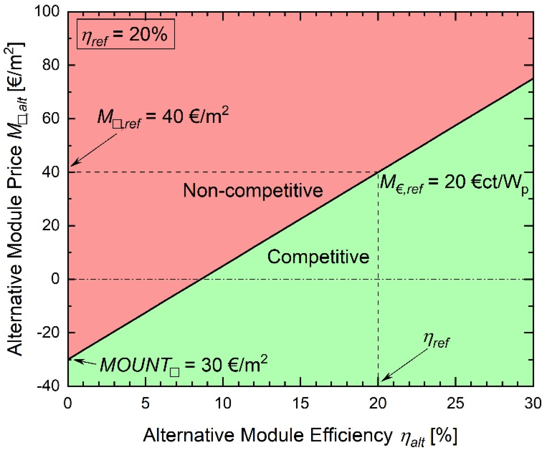
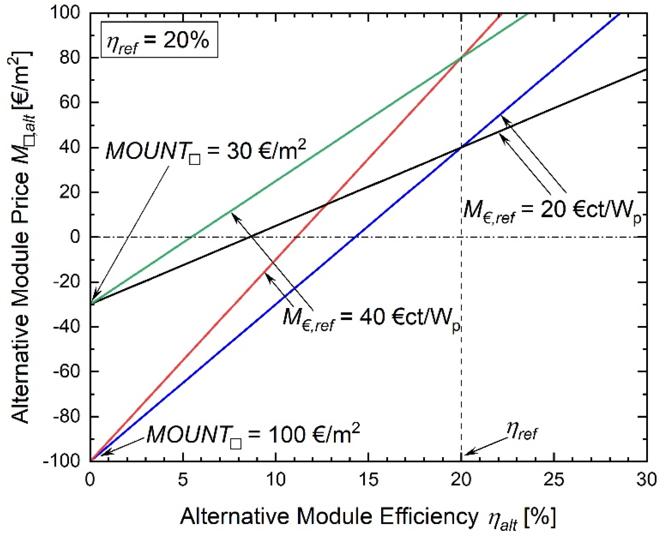
Figure 4 shows a plot of Equation (9), altered by placing an equal sign between the right-hand and left-hand sides and using MOUNT□ = 30 EUR/m2. Such mounting costs are realistic for a large area PV system as well as for small roof top systems that can be mounted easily. In some cases, the mounting costs may be even lower. Note, MOUNT□ appears as the y-axis intercept in Figure 4, and the quantity
is the slope. The value Σ□,ref in Equation (10) represents the areal cost for the complete installation of the module field: the areal purchasing price of the modules plus the cost of their full mounting.
The diagonal straight line in Figure 4 represents a decision line for an installer choosing between alternative modules. The line separates “competitive” and “non-competitive” modules. If the price for the alternative module is situated on or below the line, it represents a real alternative. However, for a module with ηalt < ηref the installer would ask for a discount △M□ from the dealer, while for ηalt > ηref the installer may be willing to pay a markup △M□. The minimal discount / maximal markup is illustrated by the diagonal line. Clearly, for the installer, modules which fall into the green area below the line are the most interesting. Consequently, for the wholesale dealer/producer, the areal sales price for a higher efficiency module must not be too high as the installer might not accept it.
From Equation (9) it follows that
Note that the acceptable module purchasing price M□,alt does not depend on the efficiency ratio ηalt/ηref alone. Instead, the installer’s decision line is dictated by:
Therefore, for installers, the mounting cost MOUNT□ is crucial, but researchers working on lower efficiency “alternative” solar cells/modules tend to overlook this matter! The second term in Equation (11) only disappears when there is a zero mounting cost, MOUNT□ = 0; then it holds M□,alt/M□,ref = ηalt/ηref for the decision line.
Figure 5 shows the decision lines derived from Equation (9) by assuming a reference efficiency ηref = 20% for two different purchasing prices and two different mounting costs MOUNT□.
4.2.1. Cut-Off Efficiency η0
At a certain cut-off efficiency η0, the decision lines in Figure 4 and Figure 5 cross the horizontal line with the value M□,alt = 0, leading to negative purchasing prices, meaning that for ηalt < η0, installers would not even take the alternative modules for free. Instead, they even ask for money to take the modules! The cut-off efficiency η0 follows from Equation (9) for M□,alt = 0 and is
For the mounting cost MOUNT□ ≈ M□,ref, it approximately holds η0 ≈ ηref/2. Thus, in the context of the present ηref ≈ 20% reference modules, any module with ηalt ≈ 10% or below would have to be given away not only for free but with additional payment for the installer—certainly not a good business model for a producer or dealer! In Figure 4, it holds η0 = 8.6%. In Figure 5, η0 ranges at 8.6% (black line), 5.4% (green line), 11.1% (red line), and 14.3% (blue line).
Figure 4 and Figure 5 explain why all silicon-based lower efficiency modules made from amorphous, microcrystalline, and even multicrystalline silicon with efficiency values below ηalt ≈ 15% dropped out of the market: given the discounts required by installers, the production costs of lower efficiency modules were simply too high as soon as alternative (mono- and multicrystalline) modules with efficiencies above 17% entered the market. Consequently, ribbon-based silicon solar cells, such as EFG cells from Schott Solar [17] and String Ribbon cells from Evergreen Solar and Sovello [18,19] disappeared from the market around 2012. The SolarWorld-owned technology of RGS-silicon [20] never entered the market at all. Similarly, numerous other technologies based on multicrystalline Si disappeared. It is also likely that, in the future, other technologies with module efficiencies below 20% will be in danger of dropping out of the market. Indeed, within the last few years even the market share of multicrystalline Si has dropped dramatically [2]. Within a few years, single crystalline silicon with module efficiencies over 20% may be all that remains.
According to Equation (9), the (negative value) of the mounting cost MOUNT□ shows up as the y-axis intercept of the diagonal lines in Figure 4 and Figure 5. Different areal prices M□,ref for the reference modules do not change the point of the y-axis intercept, but only affect the slope of the decision line. The slope in Figure 4, given by
depends on the sum of the areal purchasing price M□,ref of the modules and the total module installation cost MOUNT□, i.e., the total areal cost Σ□,ref.gen (in EUR/m2) of the fully installed PV generator using reference modules. All alternative modules with the same total areal cost Σ□,gen lie on lines parallel to those in Figure 4. Clearly, this is only made possible by a higher or lower mounting cost MOUNT□. All generators with the same MOUNT□ have the same y-axis intercept as the straight lines in Figure 4 and Figure 5, but different slopes.
4.2.2. Mark up and Discount △M□
When ηalt > ηref, dealers may request, and installers would accept, a markup in the purchasing price. When ηalt < ηref, installers may request a discount. Solving Equation (9) for the markup
one obtains
Using
for an efficiency increase (△η > 0) or reduction (△η < 0) leads to
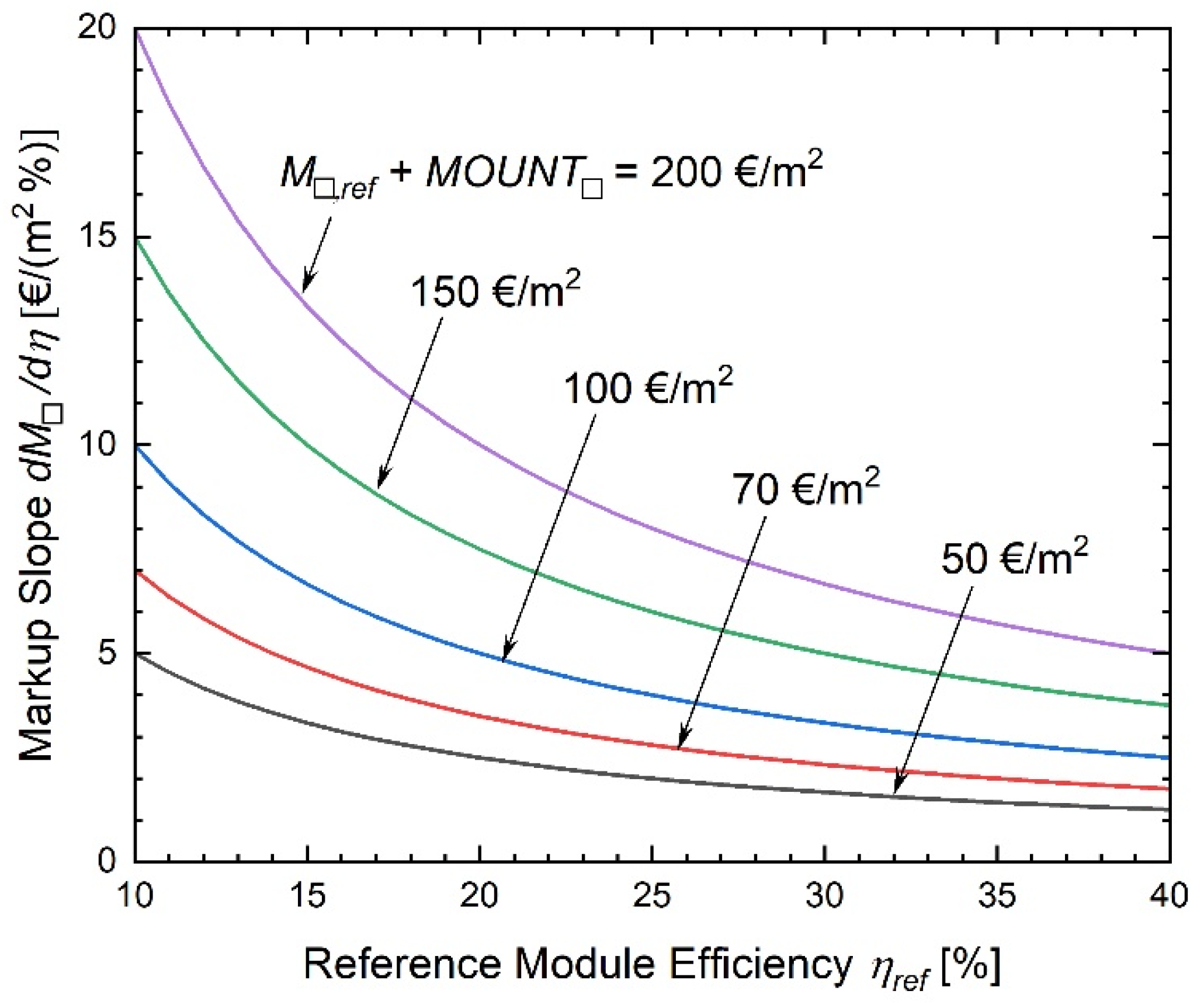
From Equation (19), we obtain the markup slope per percent efficiency increase/decrease dM□/dη = △M□/△η. This value is the same as the slope in Equation (12), namely
Figure 6 gives an example of different total installation costs Σ□, ref.gen up to a (high) value of Σ□,ref.gen. = 200 EUR/m2. The higher this value is, the higher the allowed markup that is permitted for the module producer/dealer as well as for the installer. The plot shows how much more/less alternative modules may cost if their efficiency ηalt is one absolute percentage point higher/lower than the efficiency ηref of the reference modules.
According to Equation (19), the permitted markup drops linearly with the inverse value of the reference efficiency ηref. The higher the efficiency ηref of the reference module, the smaller the slope of the markup is, this also holds when there is zero installation cost, MOUNT□ = 0. Thus, it makes a difference, if one increases the efficiency of modules from a reference efficiency ηref = 18% to ηalt = 19% or from ηref = 20% to ηalt 21%. With an increase in efficiency of one (absolute) percentage point, the permitted markup in EUR/(m2%) decreases with the inverse of the reference efficiency (if one assumes that the value of A□,ref.gen is the same for both cases). For the step from 20% to 21%, the markup is 10% less than from 18% to 19%. As shown below, the allowed markup △M€ in EUR/Wp decreases even with the square of the inverse reference efficiency ηref.
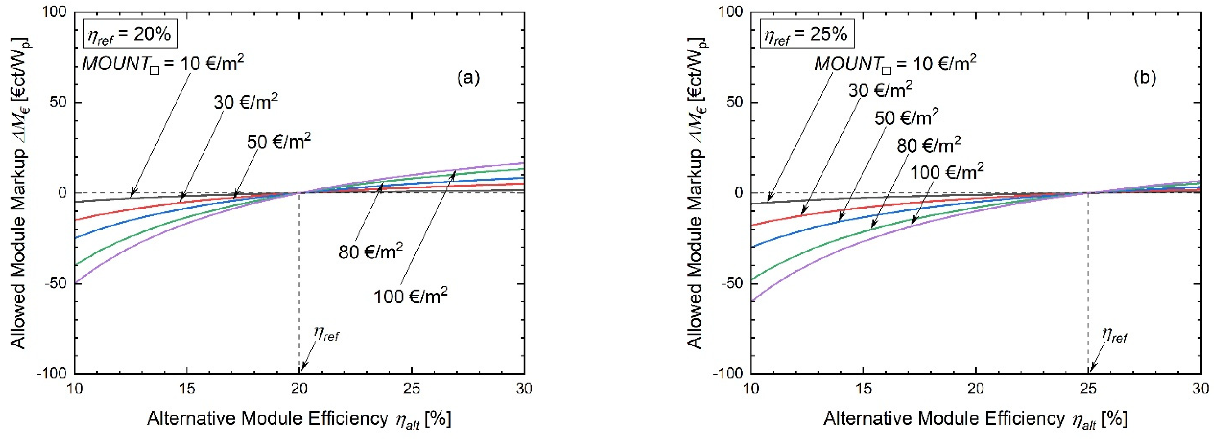
4.3. Power Related Module Decision Lines, M€
Usually, the decision between different modules is not based on area-related prices, M□, but on power-related prices, M€. The discussion of EURct/Wp or EUR/Wp makes the decision even simpler because the absolute value M€,ref of the price of the reference module does not enter into the allowed markup or discount △M€, as shown now: We insert Equations (4a) and (4b) into Equation (9) to obtain
With the markup
we obtain
Figure 7a,b show markup decision lines for reference efficiencies ηref = 20% and 25% derived from Equation (23). At present, modules with a 20% efficiency are a standard. Some producers already offer modules with a 23% efficiency and even more. The value of a 25% efficiency is chosen in Figure 7b, because, in the future, such modules must be compared with (as yet nonexistent) highly efficient silicon/perovskite tandem cell modules, with ηalt ≈ 30%. It can be seen that, depending on the mounting cost MOUNT□, the markup △M€ for these tandem cell modules would only be only a few EURct/Wp.
Inserting △η = ηalt − ηref into Equation (23) yields
For △η << ηref, it follows from Equation (24) that
Note that, compared to Equation (19), showing the area related markup △M□, in the power related markup △M€ of Equation (25), the absolute values M€,ref or M□,ref indeed do not show up. In this sense, Equation (25) is much more useful than Equation (19) to the installer making choice. Additionally, in contrast to Equation (19), in Equation (25), not only the inverse of the reference module’s efficiency ηref but the square of the inverse appears. This square immediately disappears if we convert the mounting cost per square meter, MOUNT□ to MOUNT€ via Equation (4b). It then follows from Equation (25) that
For installers, Equation (25) is more convenient to use than Equation (26) when making decisions, because the cost of mounting material (and wages) is calculated in EUR/m2 instead of EUR/Wp. In contrast, module purchasing is done in EUR/Wp.
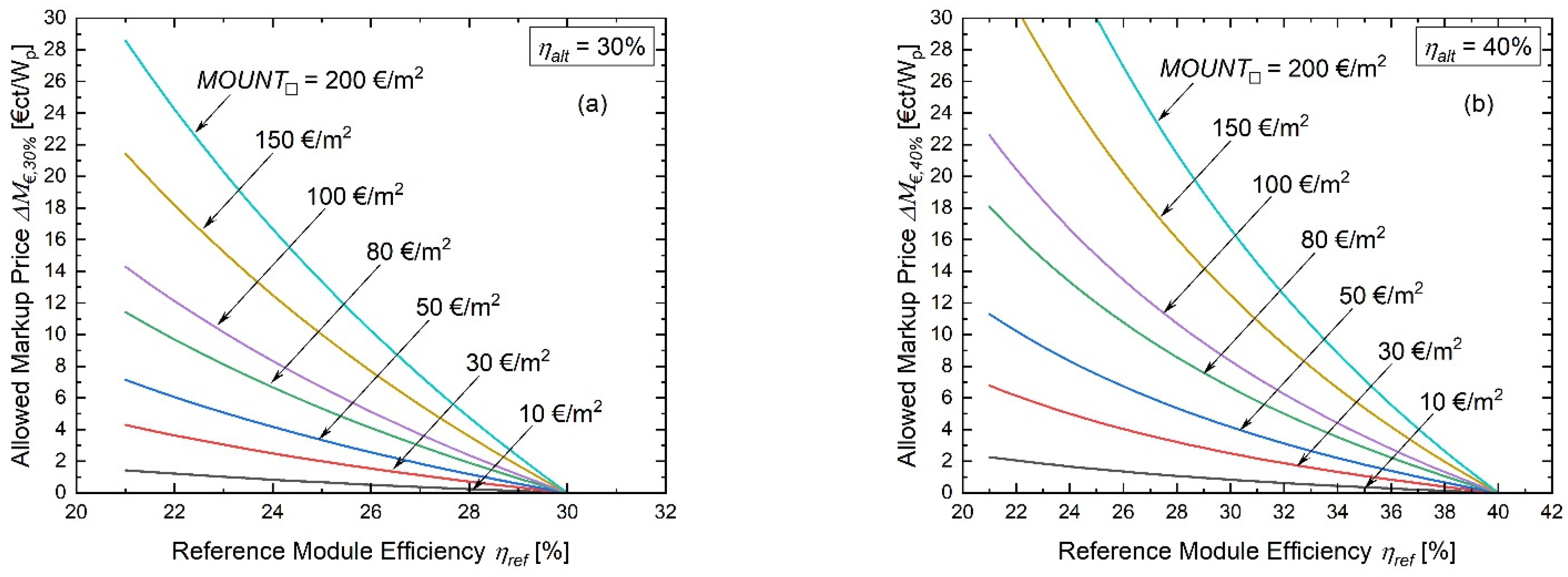
Figure 8a,b answer a slightly different question: How high the markup could be for a hypothetical tandem/triple junction module (or any other module with similarly high efficiencies) with ηalt = 30% (Figure 8a) or ηalt = 40% (Figure 8b), when compared to standard (silicon) modules with efficiencies ηref ≥ 20%? The figures show that ηalt = 30% tandem cell modules will struggle to compete against (silicon) modules with ηref = 23% efficiency (and even against ηref = 21%). The allowed markup △M€,30% for the low mounting cost MOUNT□ might be too small: For MOUNT□ = 10 EUR/m2 the 30% module must be less than △M€,30% = 1 EURct/Wp more expensive than the 23% one. Even when MOUNT□ = 50 EUR/m2, the allowed markup will be limited to approximately △M€ ≤ 6 EURct/Wp when the efficiency increases from 23% (silicon module) to 30% (future tandem cell module). With the unusually high MOUNT□ = 100 EUR/m2 one obtains △M€ ≤ 11 EURct/Wp.
This overall picture does not change much, if we consider alternative tandem/triple modules (or any other alternative technology) with efficiencies ηalt = 40%: Figure 8b demonstrates that even a module with ηalt = 40% efficiency must be still less than △M€ = 10 EURct/Wp or more expensive than one of “only” ηref = 23% efficiency when MOUNT□ ≈ 50 EUR/m2. Only when MOUNT□ > 100 EUR/m2, will the markup exceed △M€ = 15 EURct/Wp. Thus, this model, which simply considers the areal cost of “normal” installations, suggests that the market will be tough for modules containing other/more materials than crystalline silicon.
Finally, Figure 9 shows the markup slope dM€/dη for small increases in efficiency, △η << ηref, which is given by
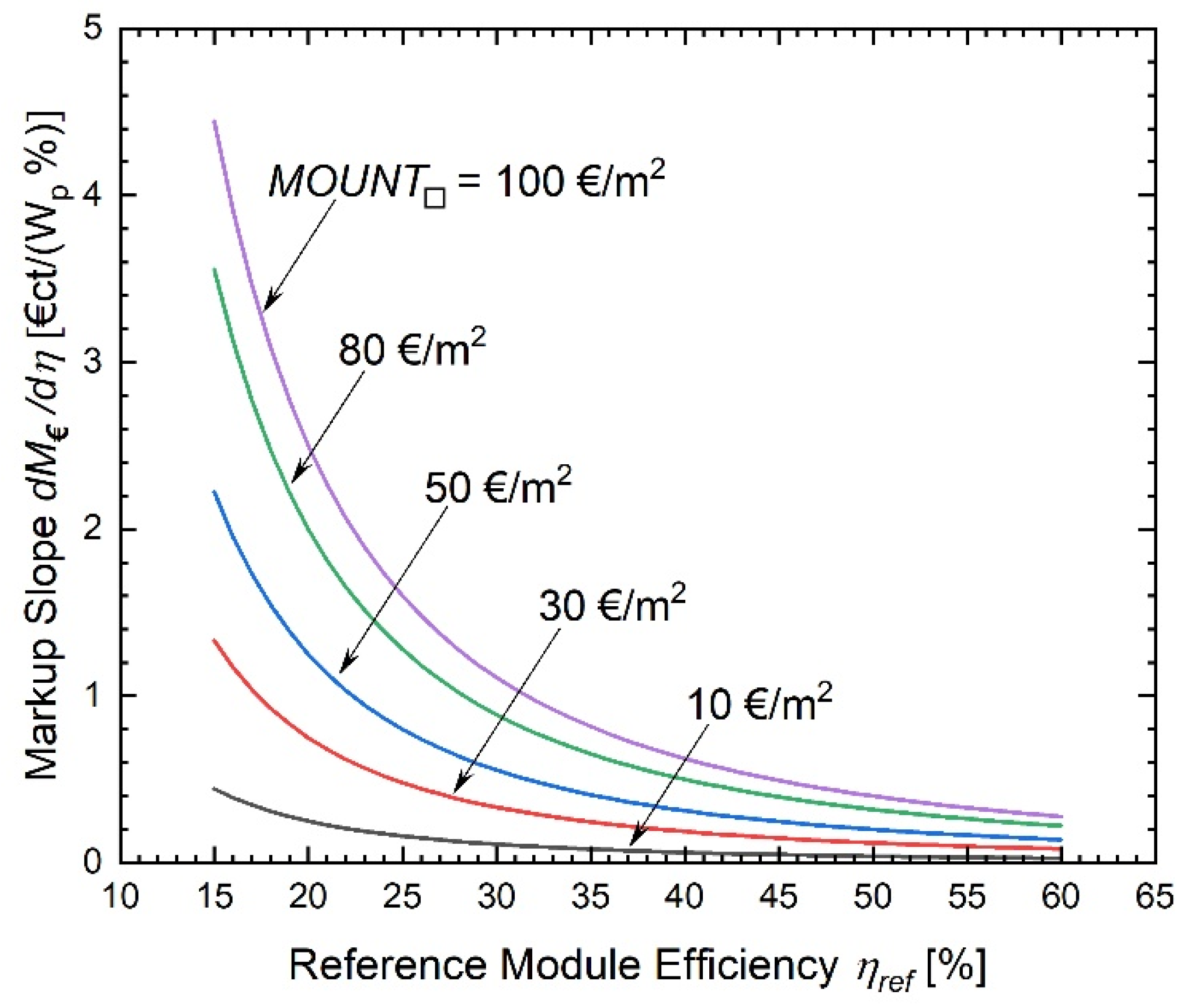
up to a 60% module efficiency. According to Equation (27), the slope of the permitted markup for alternative modules decreases with the square of the reference module’s efficiency. For example, in a case with an unusually high mounting cost MOUNT□ = 100 EUR/m2, a markup of more than 3 EURct/Wp is acceptable for an efficiency increase of 1% absolute from 20% to 21%. However, the accepted markup is only 2 EURct/Wp from 23% to 24%, and approximately 1 EURct/Wp from 30% to 31%. Furthermore, above the 40% value, the markup slope dM€/dη is far below 1 EURct/(Wp%). This must be seen in light of the fact, that above 23% to 25% module efficiency (the limit for reasonably priced, purely Si-based modules), the producers of the solar modules must have achieved a large technological advancement with huge investments, high risks, and increased operating costs at their factories. To achieve a return on their investment, producers might have to enforce much higher markup prices for higher efficiency modules in the future. It is possible that only in cases of exorbitant high installation costs, or very limited mounting areas without alternatives (such as a small roof in cases of residential applications), will installers/customers be willing to pay such high prices.
5. Conclusions
How much efficiency is enough? Certainly, from the scientific standpoint, it is interesting to attempt to increase the (monofacial) AM1.5G efficiency of solar cells and modules beyond the ηref = 25% to 26% mark that is, most probably, the upper limit for industrial, silicon-based PV modules. However, higher efficiencies require crucial technological changes, i.e., the use of either tandem cells or, another add-on (such as radiation converters?) to accompany the Si cells or alternatively, a complete replacement of Si cells. According to the model presented here, it is questionable whether the additional production costs and markups in sales prices thus required are low enough for such add-ons or replacements. The future purchasing price for a “standard” 23% to 24% efficient silicon module will probably be around 20 to 30 EURct/Wp (≈60 EUR/m2). In the long run, with the constant increases in production capacities, this price will continue to drop. Could, for example, a 30% efficient perovskite/silicon module be produced, distributed, and sold for a markup of just 6 EURct/Wp (≈18 EUR/m2)? If not, the market for utility, industrial, and residential applications might not be accessible for such modules. The opportunity seems only to be open for a rather high mounting cost MOUNT□. For all other applications, future 23% to 24% efficiency silicon-based modules (and even the present ones with 21 to 22%) might be sufficient, unless there are severe space limitations for a particular application.
Compared to increasing the efficiency of modules using (non-toxic, stable) tandem/triple cells, in many applications, it seems that it will be easier and cheaper (and at least as effective) to increase the annual yield of the complete PV system. Apart from the improvement in temperature management, bifacial modules with 10% to 30% higher annual yields are most interesting [24]: with an annual bifacial gain of 20%, future 25% efficient (monofacially measured), silicon-based bifacial modules can compete with a 30% efficiency tandem module.
Additionally, a 23% (monofacially measured) efficient Si module with 20% bifacial gain corresponds to a 28% efficient monofacial Si module with tandem cells. In fact, even with only 10% bifacial gain, such a 23% efficient bifacial module, can compete with a future (probably high priced) 25% efficient monofacial module. The technologies required for such inexpensive bifacial modules exist already today: The ZEBRA technology of the ISC Konstanz [25], for example, combines the low-cost production of bifacial, back side contact cells/modules with a high annual yield.
Finally, we consider: How much efficiency is necessary? Is 20% also enough? For most future applications, the answer will probably be “no!”. In light of the arguments given above, installers will ask for (probably high) discounts if they are required to accept modules with efficiencies below the future “standard”, i.e., 23% efficiency Si modules. It is hard to imagine that large-area secondary photovoltaics modules made from CdTe or Cu(In,Ga)Se2, or from organic semiconductors will ever reach this level in mass production. These technologies may have the same destiny as amorphous, microcrystalline, and multicrystalline Si. The module efficiencies of all these technologies are inherently limited by electronic defects, and, in addition by inhomogeneities, as was first discussed in Ref. [26] on the cell level. In thin film/secondary photovoltaic modules, the consequences of spatial inhomogeneities and local differences in cell efficiencies are much more severe than for modules made from single crystalline Si. Due to their seemingly elegant production technology involving the integrated series connection within thin film modules, cells in such modules cannot be sorted anymore after their production. Therefore, the overall module efficiency is limited by the cells with the lowest quality. In the “old fashioned” wafer-based Si technology, the cells can be sorted (usually in four bins) and modules with a tailored efficiency are fabricated. “Lower” efficiency cells are simply sorted out (and either recycled/remelted or cut into smaller cells, which end up in garden lamps etc.). Therefore, even if thin-film cells, e.g., from perovskites, ever will come close or even exceed the efficiency of single crystalline Si cells on (a small-area) cell level, it will be hard to outperform wafered Si on the module level, due simply to the integrated series connection. Unfortunately, installers are not interested in the physical reasons for lower efficiency, they simply ask for a price discount.
Thus, does it make sense to pursue research on other photovoltaic materials besides silicon? The answer is both yes and no! From the scientific point of view, it is certainly interesting. However, economically, the only technologies that seem interesting are those that can be added on to the present and future highly efficient silicon cells and modules. The fight against climatic change can only be sustained with silicon-based modules. All other activities will not only be too late (and sometimes even too toxic), but they might also be too expensive for the large-area, low-cost, CO2-free generation of electricity, given the future requirement of hundreds of TWp of installed PV power.
Funding
This research received no external funding.
Acknowledgments
The author gratefully acknowledges the indispensable help of Yanqiu Zhao with the drawings, fruitful discussions with Michael Reuter (Solarzentrum Stuttgart GmbH), Salentino Primitivo di Manduria (JHW Consulting Ltd.), Roman Jehle (Actensys GmbH), Radovan Kopecek (Institute for Solar Energy, Konstanz), as well as with Renate Zapf-Gottwick and Michael Saliba, both from the Institute for Photovoltaics, University of Stuttgart.
Conflicts of Interest
The author declares no conflict of interest.
References and Notes
- Chapin, D.M.; Fuller, D.S.; Pearson, G.L. A New Silicon p-n Junction Photocell for Converting Solar Radiation into Electrical Power. J. Appl. Phys. 1954, 25, 676. [Google Scholar] [CrossRef]
- Philipps, S.; Warmuth, W. Photovoltaics Report. Available online: https://www.ise.fraunhofer.de/de/veroeffentlichungen/studien/photovoltaics-report.html (accessed on 11 February 2022).
- Jäger-Waldau, A. Snapshot of Photovoltaics—March 2021. EPJ Photovolt. 2021, 12, 2. [Google Scholar] [CrossRef]
- Werner, J.H. Second and Third Generation Photovoltaics—Dreams and Reality. In Advances in Solid State Physics; Kramer, B., Ed.; Springer: Berlin/Heidelberg, Germany, 2004; Volume 44, pp. 51–66. [Google Scholar] [CrossRef]
- Bergmann, R.B.; Werner, J.H. The future of crystalline silicon films on foreign substrates. Thin Solid Film 2002, 403–404, 162–169. [Google Scholar] [CrossRef]
- Jackson, P.; Würz, R.; Rau, U.; Mattheis, J.; Kurth, M.; Schlötzer, T.; Bilger, G.; Werner, J.H. High quality baseline for high efficiency Cu(In1-x, Gax) solar cells. Prog. Photovolt. 2007, 15, 507–519. [Google Scholar] [CrossRef]
- Green, M.A. Third Generation Photovoltaics; Springer: Berlin/Heidelberg, Germany, 2003; ISBN 3540401377. [Google Scholar]
- Marti, A.; Luque, A. Next Generation Photovoltaics—High Efficiency through Full Spectrum Utilization; Institute of Physics Publishing: Bristol, UK, 2004; ISBN 0750309059. [Google Scholar]
- Saliba, M.; Correa-Baena, J.-P.; Wolff, C.M.; Stolterfoht, M.; Phung, N.; Albrecht, S.; Neher, D.; Abate, A. How to make over 20% Perovskite Solar Cells in Regular (n-i-p) and Inverted (p-i-n) Architectures. Chem. Mater. 2018, 30, 4193–4201. [Google Scholar] [CrossRef]
- Zhang, Y.; Park, N.-G. Quasi-Two-Dimensional Perovskite Solar Cells with Efficiency Exceeding 22%. ACS Energy Lett. 2022, 7, 757–765. [Google Scholar] [CrossRef]
- Luceno-Sanchez, J.A.; Diez-Pacual, A.M.; Capilla, R.P. Materials for Photovoltaics: State of the Art and Recent Developments. Int. J. Mol. Sci. 2019, 20, 976. [Google Scholar] [CrossRef] [PubMed] [Green Version]
- Werner, J.H.; Kolodinski, S.; Queisser, H.J. Novel optimization principles and efficiency limits for semiconductor solar cells. Phys. Rev. Lett. 1994, 72, 3851–3854. [Google Scholar] [CrossRef] [PubMed]
- Available online: https://www.pv-magazine.com/2021/06/02/longi-achieves-25-21-efficiency-for-topcon-solar-cell-announces-two-more-records (accessed on 17 February 2022).
- Yoshikawa, K.; Kawasaki, H.; Yoshida, W.; Irie, T.; Konishi, K.; Nakano, N.; Uto, T.; Adachi, D.; Kanematsu, M.; Uzu, H.; et al. Silicon heterojunction solar cell with interdigitated back contacts for a photoconversion efficiency over 26%. Nat. Energy 2017, 2, 17032. [Google Scholar] [CrossRef]
- Richter, A.; Hermle, M.; Glunz, S.W. Reassessment of the Limiting Efficiency for Crystalline Silicon Solar Cells. IEEE J. Photovolt. 2013, 3, 1184–1191. [Google Scholar] [CrossRef]
- Luo, W.; Khoo, Y.S.; Hacke, P.; Naumann, V.; Lausch, D.; Harvey, S.P.; Singh, J.P.; Chai, J.; Wang, Y.; Aberle, A.G.; et al. Potential-induced degradation in photovoltaic modules: A critical review. Energy Environ. Sci. 2017, 10, 43–68. [Google Scholar] [CrossRef] [Green Version]
- Kales, J.; Schmidt, W.; Schwirtlich, I.; Hoffmann, W. Challenges for EFG ribbon technology on the path to large scale manufacturing. In Proceedings of the Record of the Thirty-First IEEE Photovoltaic Specialists Conference, Lake Buena Vista, FL, USA, 3–7 January 2005; pp. 1301–1304. [Google Scholar]
- Available online: https://en.wikipedia.org/wiki/Evergreen_Solar (accessed on 17 February 2022).
- Hahn, G.; Hauser, A.; Gabor, A.M.; Cretella, M.C. 15% efficient large area screen printed string ribbon colar cells. In Proceedings of the Conference Record of the Twenty-Ninth IEEE Photovoltaic Specialists Conference, New Orleans, LA, USA, 19–24 May 2002; pp. 182–185. [Google Scholar] [CrossRef] [Green Version]
- Lange, H.; Schwirtlich, I.A. Ribbon Growth on Substrate (RGS)—A new approach to high speed growth of silicon ribbons for photovoltaics. J. Cryst. Growth 1990, 104, 108–112. [Google Scholar] [CrossRef]
- The price for an own purchase in 2020 for 1000 wafers, high lifetime, n-Type, single Crystalline Si, Was 20 €/m².
- Deutsche Gesellschaft für Sonnenenergie. Planning and Installing Photovoltaic Systems—A Guide for Installers, Architects, and Engineers, 3rd ed.; Routledge: Abdingson, UK, 2013; p. 189. [Google Scholar]
- f = 40% means that the ratio of the (slanted) PV generator’s area to the base area of the land is 40%.
- Kopecek, R.; Libal, J. Bifacial Photovoltaics 2021: Status, Opportunities and Challenges. Energies 2021, 14, 2076. [Google Scholar] [CrossRef]
- Kopecek, R.; Libal, J.; Lossen, J.; Mihailetchi, V.D.; Chu, H.; Peter, C.; Buchholz, F.; Wefringhaus, E.; Halm, A.; Ma, J.; et al. ZEBRA technology: Low cost bifacial IBC solar cells in mass production exceeding 23.5%. In Proceedings of the 2020 47th IEEE Photovoltaic Specialists Conference (PVSC), Calgary, AB, Canada, 15 June–21 August 2020; pp. 1008–1012. [Google Scholar] [CrossRef]
- Werner, J.H.; Mattheis, J.; Rau, U. Efficiency limitations of polycrystalline thin film solar cells: Case of Cu(In,Ga)Se2. Thin Solid Films 2005, 480–481, 399–409. [Google Scholar] [CrossRef]
Figure 1.
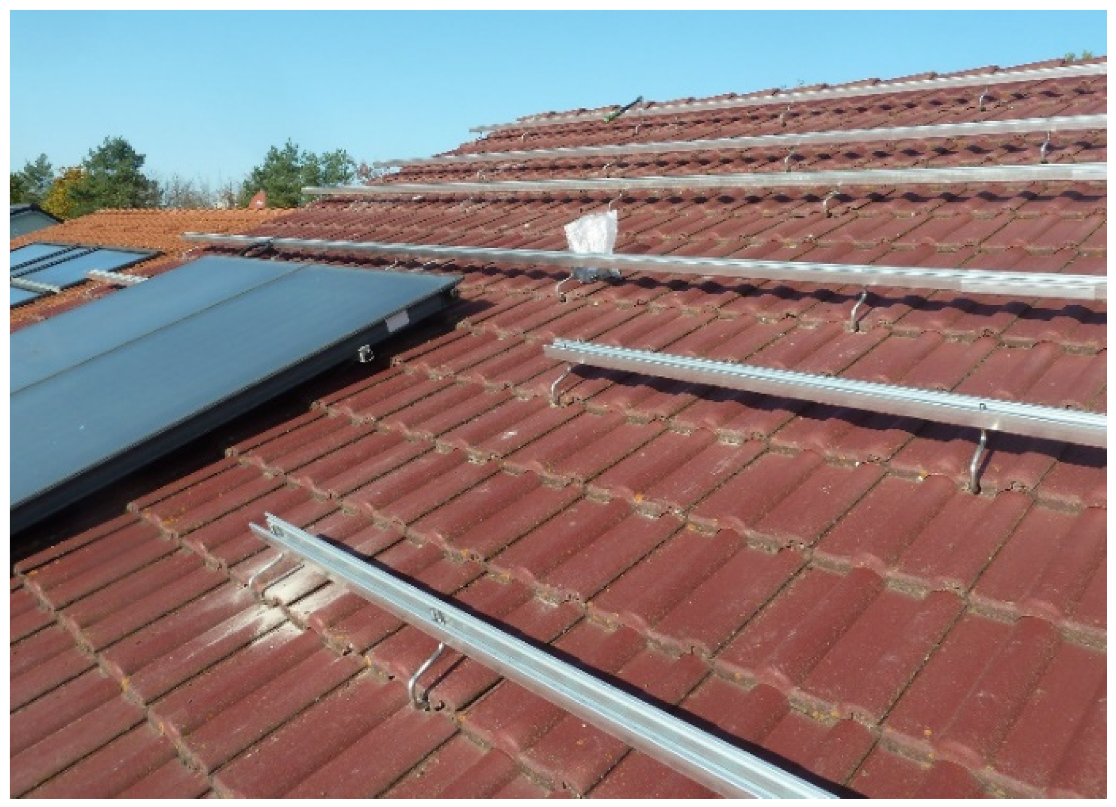
Mounting/railing system for a relatively simple 11 kWp, residential PV generator on a tiled roof. The roof angle is 25°. Only the two solar thermal collectors on the lefthand side cannot be covered by PV modules. Including wages, the total mounting cost ranged at MOUNT□ ≈ 40 EUR/m2. Due to the necessary, but time-consuming, process of cutting/adjusting tiles for the roof hooks, this mounting cost is relatively high.
Figure 1.
Mounting/railing system for a relatively simple 11 kWp, residential PV generator on a tiled roof. The roof angle is 25°. Only the two solar thermal collectors on the lefthand side cannot be covered by PV modules. Including wages, the total mounting cost ranged at MOUNT□ ≈ 40 EUR/m2. Due to the necessary, but time-consuming, process of cutting/adjusting tiles for the roof hooks, this mounting cost is relatively high.

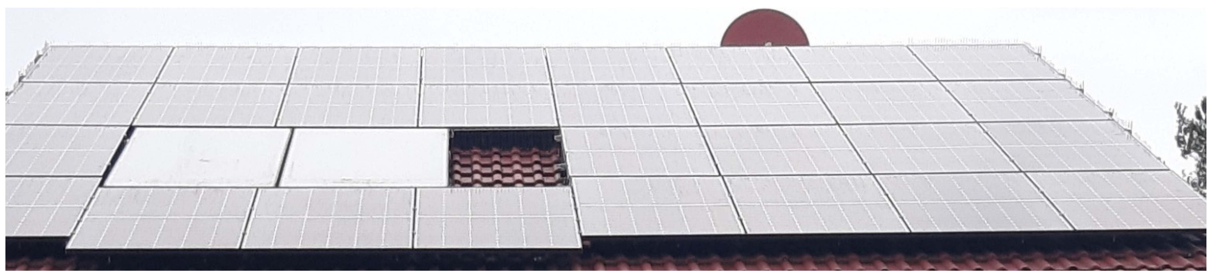
Figure 2.
The 11 kWp PV generator after installation. It consists of 29 PV modules mounted around two solar thermal collectors.
Figure 2.
The 11 kWp PV generator after installation. It consists of 29 PV modules mounted around two solar thermal collectors.

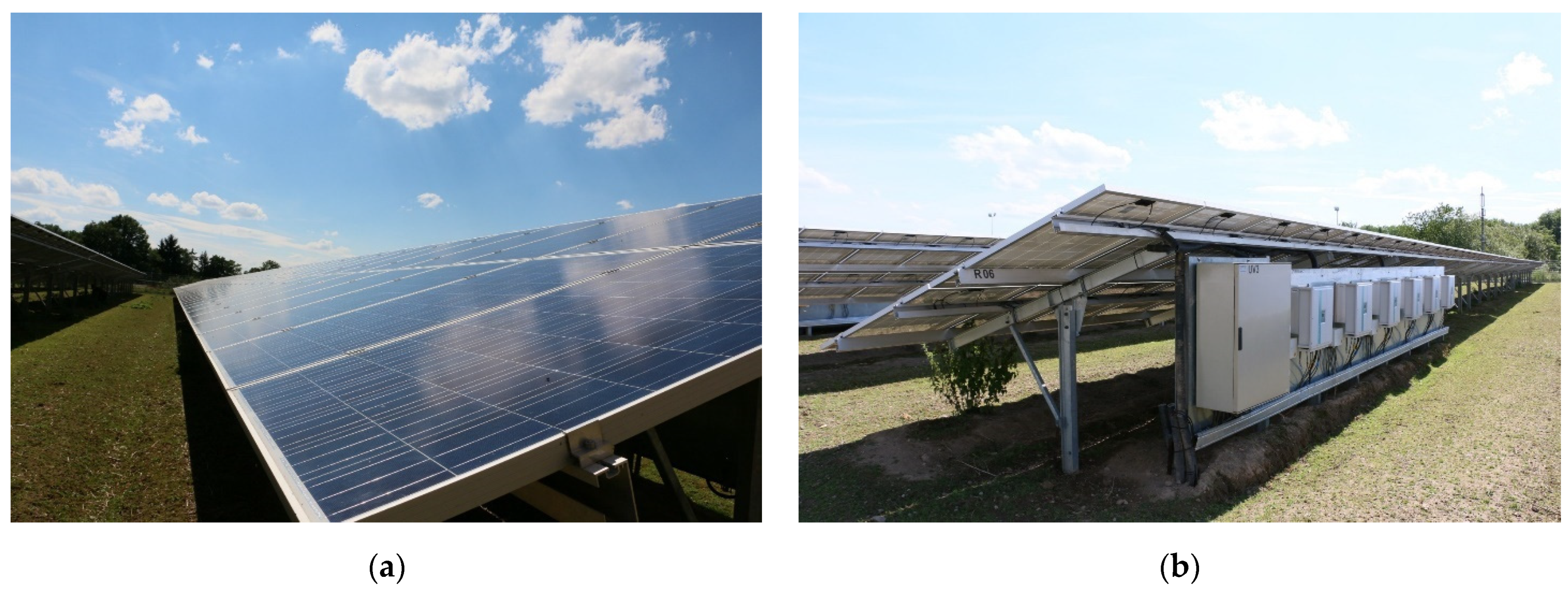
Figure 3.
A 200 kWp PV system mounted in 2013. (a) Front view with multicrystalline Si modules. (b) Back view. The mounting system, contributing to the mounting cost MOUNT, employed in Equation (2), consists of piled steel poles and steel rails. The six inverters and the large box for housing the internet connection are included in the FIX in Equation (2). The total mounting cost was MOUNT□ ≈ 35 EUR/m2.

Figure 4.
Module decision line from Equation (9) with an assumed reference efficiency ηref = 20% and mounting cost MOUNT□ = 30 EUR/m2. The assumed M€,ref = 20 €ct/Wp for the reference modules corresponds to M□,ref = 40 EUR/m2. For the installer, the diagonal line divides the available modules offers into competitive and non-competitive. Modules with efficiencies η < η0 = 8.6% (cut-off efficiency) are below the zero line and would have to be sold for negative prices!

Figure 5.
Module decision lines for reference modules with ηref = 20% and purchasing prices of either M€,ref = 20 EURct/Wp or M€,ref = 40 EURct/Wp, and installation cost of either MOUNT□ = 30 EUR/m2 or (unusually high) MOUNT□ = 100 EUR/m2. Only alternative modules falling either onto or below the lines are interesting for installers.

Figure 6.
Slope of the module decision lines with differently assumed efficiencies for the reference modules and different total cost for the complete generator field (areal costs of modules plus mounting cost) derived from Equation (20). The higher the reference modules’ efficiency ηref, the smaller the permitted areal markup for alternative modules per each singular (absolute) percentage point increase in efficiency.

Figure 7.
Markup decision lines for alternative modules, when the reference modules have (a) ηref = 20% and (b) ηref = 25% efficiency. Different mounting costs MOUNT□ are considered. Only alternative modules lying below the decision lines are economically interesting for the installer. Compared to the present price of approximately 30 EURct/Wp for modules with ηref ≈ 21% efficiency, the markup permitted for modules with alternative efficiencies ηalt > ηref is quite small, especially in the case of a low mounting cost MOUNT□.

Figure 8.
Allowed markup of new, hypothetical alternative modules with assumed efficiencies (a) ηalt = 30% and (b) ηalt = 40%, compared to lower efficiency modules. (a) For a typical mounting cost MOUNT□ < 50 EUR/m2, the hypothetical 30% efficiency module only has an acceptable markup △M€,30% ≤ 6 EURct/Wp when compared to a future (silicon) standard module with ηref = 23% efficiency. (b) Even for a hypothetical module with ηalt = 40%, the accepted markup is around △M€,40% ≤ 10 EURct/Wp when compared to a ηref = 23% reference module and at △M€,40% ≤ 13 EURct/Wp when compared to today’s standard 20 to 21% efficient silicon modules. Future, high-efficiency modules are only competitive when high mounting costs are involved.

Figure 9.
Data derived from Equation (27). Slopes of the module decision lines such as those in Figure 7a,b. The higher the reference modules’ efficiency ηref, the smaller the markup per each singular absolute percentage point in efficiency increase.
Figure 9.
Data derived from Equation (27). Slopes of the module decision lines such as those in Figure 7a,b. The higher the reference modules’ efficiency ηref, the smaller the markup per each singular absolute percentage point in efficiency increase.


Table 1.
Areal price of PV modules in comparison to other construction materials. The PV-modules fall in the same price range as clay-based brick stones. Shown as well are the required prices for modules with efficiencies of 10% and 5%, which would produce the same power as the 20% efficiency module. Even without considering the mounting cost, the low efficiency modules are not competitive.
| Construction Material | Price [EUR/m2] | Required Price η = 10% [EUR/m2] | Required Price η = 5% [EUR/m2] |
|---|---|---|---|
| η = 20% module; M€ = 20 EURct/Wp | 40 | 20 | 10 |
| M€ = 40 EURct/Wp | 80 | ||
| Simple windows with two glasses | 100–300 | ||
| Stainless steel sheets, 1 mm | 70–150 | ||
| Brick stones | 40–80 | ||
| Steel sheets, 1 mm | 30–50 | ||
| Ceramic tiles | 10–50 | ||
| High lifetime Si wafers | 15–30 | ||
| Window glass | 5–20 | ||
| Block board, 18 mm | 10–25 | ||
| Ingrain wallpaper | 0.5–1 |
Table 2.
Gross cost estimation for roof or ground mounted grid connected PV-systems in the power range 10 kWp < PPV < 1000 kWp. All values stem either from personal communications with installers or from the author’s own installations. Note that the lowest/highest price of one item almost never occurs together with the lowest/highest prices of the other two items. For example, a low module purchasing price M with a quantity discount for the large number of modules required for large area PV systems does not necessarily accompany a low MOUNT and low FIX. For example, machines for structural engineering and transformers to facilitate the connection to the medium-voltage grid might be necessary. A margin for the installer(s) (for example of 5% for a large area ground mounted system or 20 to 30% for a small residential roof-top system) is not included. The data apply to a completely installed grid-connected system in Germany.
| Installation Cost of PV System | EUR/m2 | EUR/kWp | Percentage [%] |
|---|---|---|---|
| Module purchasing price M, η = 20% | 40–80 | 200–400 | 20–40 |
| Balance of systems BOS = MOUNT + FIX | |||
| Module mounting cost MOUNT (material + labor) | 20–100 | 100–500 | 20–40 |
| 200–700 | 20–60 | |
| Total TEUR | 700–1500 | 100 |
Publisher’s Note: MDPI stays neutral with regard to jurisdictional claims in published maps and institutional affiliations. |
© 2022 by the author. Licensee MDPI, Basel, Switzerland. This article is an open access article distributed under the terms and conditions of the Creative Commons Attribution (CC BY) license (https://creativecommons.org/licenses/by/4.0/).
Share and Cite
MDPI and ACS Style
Werner, J.H. How Much Photovoltaic Efficiency Is Enough? Solar 2022, 2, 215-233. https://doi.org/10.3390/solar2020012
AMA Style
Werner JH. How Much Photovoltaic Efficiency Is Enough? Solar. 2022; 2(2):215-233. https://doi.org/10.3390/solar2020012
Chicago/Turabian StyleWerner, Jürgen Heinz. 2022. "How Much Photovoltaic Efficiency Is Enough?" Solar 2, no. 2: 215-233. https://doi.org/10.3390/solar2020012