1. Introduction
A key factor for the continuous photovoltaic (PV) technology uptake is the reduction of its levelized cost of electricity (LCOE). This can be achieved by increasing lifetime performance through advanced monitoring that provides quality control through data-driven predictive performance and cost-effective operation and maintenance (O&M). In this domain, monitoring systems can assist in improving the reliability and service performance of PV systems by enhancing existing functionalities with next-generation data-driven operational-state and performance verification solutions [
1]. Such features include data quality routines (DQRs) for data validity and sanity [
2], system health-state predictive models offering events-driven operational state information, and failure diagnosis routines (FDRs) for the timely detection of faults. The integration of such functionalities for monitoring system architectures ensures optimal levels of PV performance by mitigating power losses due to operational problems and reducing system’s downtime [
3].
At present, most PV installations are by default monitored either via inverter-based solutions (i.e., passive monitoring systems) or through active monitoring systems. Inverter-based monitoring systems perform basic PV performance and measurements checks. Such functional systems are integrated in inverters and alert operators when an inverter is underperforming. Additionally, grid errors (e.g., inverter disconnection, damaged AC cable), errors at the AC side, unstable PV operation (e.g., near zero DC power production), sensors errors (e.g., communication fault with the meter unit), ground faults, and other incidents (such as inverter over-temperature, DC overvoltage, and overcurrent) can be detected. However, passive monitoring systems often trigger false alerts, especially during cloudy days, and they cannot detect faults that cause a small amount of power loss nor PV array-related problems.
Recent advancements in monitoring solutions that support high plant performance are associated with the so-called active monitoring systems, which integrate data-driven algorithms for PV performance assessment and fault detection at the array and string level [
1]. To this end, the current advances in the field of machine learning and the rapid developments of artificial intelligence (AI) enable novel features to be integrated into active PV monitoring systems. Such functionalities entail the predictive ability of machine learning and the diagnostic power of AI to overcome data processing and mining issues, and to capture the actual behavior of PV systems for effective predictive maintenance. Some of them offer remote diagnosis of failures in PV systems based on Internet of Things (IoT) [
4], cloud-computing [
5], and satellite observations [
6]. Other approaches employ machine learning techniques to simulate the PV performance and extract useful information from the available measurements and decide upon underperformance conditions [
7]. Moreover, these systems apply different threshold levels (TL) [
8], either static or dynamic, for determining whether the system is performing as expected or not, also offering constant alerting in case of malfunctions and system underperformance [
9].
Over the past years, numerous algorithms have been presented to address the challenges of accurately detecting PV system faults and to form foundational parts of health-state architectures applicable to monitoring systems. Health-state monitoring refers to the data-driven strategies applied to improve the performance and reliable operation of PV systems. Overall, the basis of most presented methods is the comparative analysis of historical or predicted performance to actual data and the identification of fault signatures [
10] through abnormal data patterns by applying statistical [
11] or machine learning techniques [
12].
With respect to the failure detection at the PV array level, most published failure detection routines define operational range limits for each monitored parameter and make a decision on the fault condition when measured values exceed a threshold limit [
13]. Other studies utilized both univariate and multivariate statistical outlier detection techniques [
14] to detect failures from the comparison of the actual and predicted PV system performance [
15,
16]. In this context, the application of machine learning power output predictive models is rapidly evolving due to the enhanced accuracy and robustness offered compared to other deterministic approaches. Moreover, by leveraging machine learning principles, the technical bottlenecks arising from the lack of PV system metadata (e.g., installation characteristics and operational performance status) are overcome since the performance is entirely captured from historic data [
17]. Despite a multitude of employed techniques and studies in the area of fault detection, a main challenge remains the lack of a unified approach for robust and scalable PV system health-state architecture. In addition, the diagnostic accuracy of failure detection models is dependent on the availability and quality of site-specific historical data as well as on the performance accuracy of the predictive model [
18]. Moreover, the prediction model selection is an area that is not yet fully explored due to lack of well-defined methodologies and standardization for deriving the most appropriate model [
18].
A unified PV system health-state architecture that comprises of data-driven functionalities is presented in this work. The main contribution lies in the combination of regression and classification models for PV system health-state assessment based on eXtreme Gradient Boosting (XGBoost) with the ability to predict power output and to detect data issues and typical power-related faults. The analysis aims to fill in the gap of knowledge by presenting a methodology for developing a PV system health-state architecture by leveraging the XGBoost algorithm and constructing optimally performing predictive and classification models. The approach for the development of the predictive model relies on optimized model hyper-parameters by following structured supervised learning regimes that utilize low partitions of historic data and input features for the training procedure. In case of field data unavailability, a synthetic generated PV dataset (using measured meteorological data) can be used for its development. Concurrently, XGBoost was used to construct a fault classifier for the categorization of PV operating conditions (i.e., normal and fault conditions). The training regime was based on either field or synthetic generated data and reinforced using a resampling technique to improve the classifiers’ accuracy. The effectiveness of the health-state architecture was experimentally validated using three different PV datasets: (a) a dataset containing historic performance measurements with/without fault patterns of 5% relative power reduction, (b) a synthetic generated dataset with/without fault patterns of 5% relative power reduction, and (c) a dataset containing historic field-emulated failures. All datasets were obtained from a test-bench PV system installed in Nicosia, Cyprus.
Additionally, the health-state architecture includes implemented routines that comprise of a sequence of data filters and statistical comparisons applied to acquire performance data to detect erroneous data (attributed to faults of communication, sensor, and data-acquisition devices). Lastly, the implemented routines and the proposed architecture provide useful information to PV power plant operators regarding modeling approaches for the timely detection of faults and uninterrupted monitoring of PV systems.
2. Materials and Methods
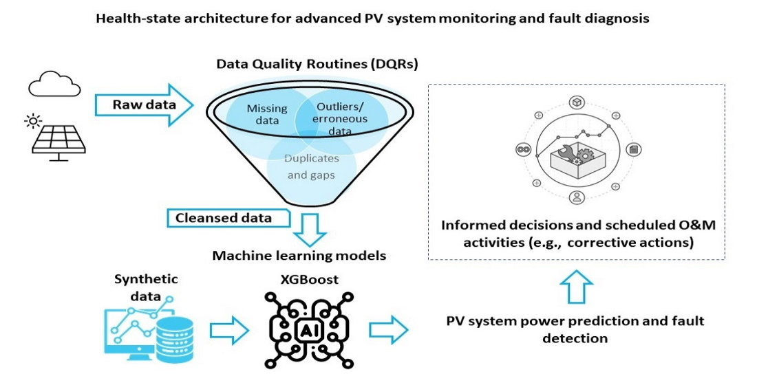
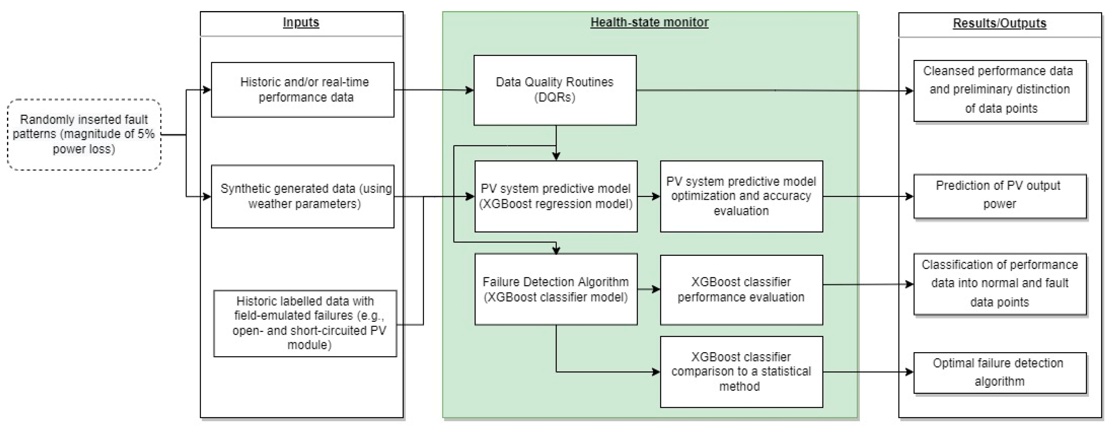
This section describes the experimental setup and the methodological approach of the proposed health-state architecture for PV systems, which is conceptualized to operate on field performance data (i.e., historic or real-time meteorological and electrical measurements). The raw data are first filtered using DQRs to evaluate their quality and provide cleansed data. A data-driven predictive model is then constructed using different model construction conditions (i.e., input features, partitions of actual and synthetic generated performance data for the training procedure, etc.) to simulate the PV performance using an XGBoost regression model. The ultimate scope of this procedure is to develop an accurate predictive model that would utilize low shares of data and commonly monitored input features. In case of measured data unavailability, a synthetic generated PV dataset (using measured meteorological data from the test PV installation) can be used for the development of the predictive model. The model’s accuracy is finally evaluated using a yearly PV dataset, containing 15-min field measurements obtained from a test-bench PV system installed in Nicosia, Cyprus.
Further to the PV predictive model, a fault detection stage is proposed to complement a sound health-state architecture. In this stage, a classifier using XGBoost is proposed to determine underperformance incidents (that cause reduction in power measurements) in PV systems. To evaluate its performance, fault conditions were introduced to both the actual and synthetic generated PV datasets. The fault conditions were randomly imputed by reducing the power measurements magnitude to a relative level of 5%. Each fault condition point was labeled in order to be used in a supervised learning regime to construct a fault detection classifier. The performance of the developed classifier was evaluated under these fault conditions, and it was then compared against a statistical method.
Finally, to demonstrate the applicability of the health-state architecture for detecting faults in operating PV systems, a time series with historic field-emulated failures from the test-bench PV system was used. The functional block diagram of the proposed health-state architecture is illustrated in
Figure 1.
2.1. Experimental Setup
Historical field measurements were obtained from a test-bench PV system installed in Nicosia, Cyprus (Köppen-Geiger-Photovoltaic climate classification CH; steppe climate with high irradiation) [
19]. The array includes five crystalline-Silicon (c-Si) modules (connected in series) and is installed in an open-field mounting arrangement at an inclination angle of 27° due South [
20]. The system is grid-connected with a total capacity of 1.2 kW
p.
A data-acquisition (DAQ) platform is used for the monitoring and storage of meteorological and electrical measurements. The monitoring is performed following the requirements of the IEC 61724-1 [
21]. The meteorological measurements include the in-plane irradiance
, ambient temperature
, wind speed
, and direction
. The PV operational data include the back-surface module temperature
, array DC current
, and voltage
multiplied together to calculate the DC power
and AC output power
. Additional yields and performance metrics such as the array energy yield
, the final PV system yield (
), the reference yield (
), and the performance ratio (
) were also calculated [
22]. The solar position parameters of solar azimuth
and elevation
angles were finally calculated using solar position algorithms [
23]. The system was continuously monitored and high-quality data (at a resolution of 1 s and recording interval of 1-, 15-, 30-, and 60-min averages) were acquired over a yearly evaluation period.
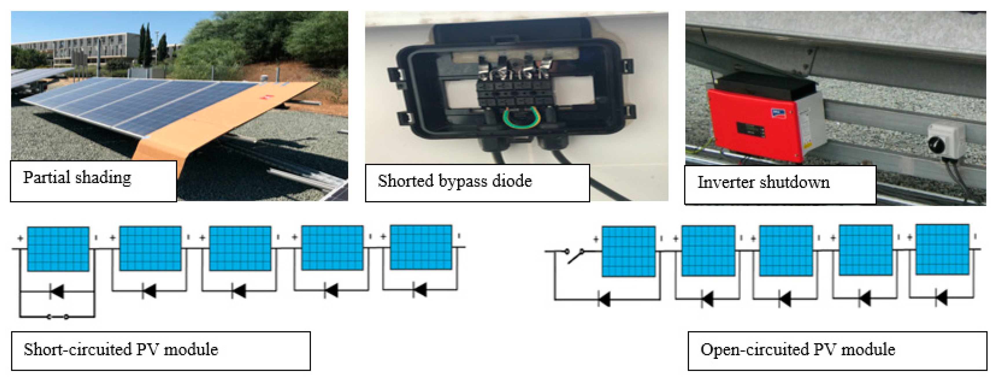
The maintenance and cleaning of the PV array and the pyranometer were carried out on a seasonal basis (i.e., four cleaning events per year) and after dust events to minimize any soiling effects. Systematic recalibration of the sensors was performed as specified by the manufacturers, and periodic cross-checks against neighboring sensors (other pyranometers and temperature sensors installed in close proximity) were conducted to identify sensor drifts. During the system’s operation, different types of failures (e.g., open- and short-circuited PV module, inverter shutdown, shorted bypass diode, partial shading), data issues (e.g., communication loss, sensors faulty operation, missing and erroneous data values, etc.) and maintenance events occurred and information about the incidents (outage’s periods and actual failure sources) and performed actions were kept in maintenance logs.
2.2. Actual and Synthetic Performance Datasets
The actual electrical and weather data acquired for the test-bench PV system were aggregated as 15-min averages over a yearly evaluation period (from June 2015 to June 2016) and used to create the actual performance time series (also referred to as the yearly actual PV dataset). The constructed time series was used for both the predictive and classification model development, as well as for the validation procedure of the architecture for diagnosing fault conditions in PV systems.
In parallel, a synthetic performance time series over a period of a year was generated by inputting the 15-min meteorological measurements from Nicosia, Cyprus, and system-specific metadata to the Sandia PV Array Performance Model (SAPM) [
24], available in pvlib-Python [
25]. The synthetic generated time series replicates the operation of the test-bench PV system and was used to facilitate the evaluation of the classification model.
2.3. Fault Conditions Introduction and Emulation Procedure
To evaluate the performance of the health-state architecture for classifying normal and fault conditions in PV systems, fault patterns were introduced to both the actual and synthetic PV datasets by declining the array DC power at a relative magnitude of 5% for occurrences at high irradiance conditions (over 600 W/m
2). As reported by the International Energy Agency (IEA) in the report outlying the PV module failures [
26], the minimum detection limit for power loss is 3%. Furthermore, detectable PV module failures (i.e., short-circuited and inverted bypass diode, short-circuited and cracked cells, light-induced degradation, corrosion, delamination, etc.) cause power loss higher than 2% [
26]. To distinguish fault events (e.g., partial shading, bypass diode faults, etc.) from degradation modes (e.g., corrosion of the antireflection coating, initial light-induced degradation, glass corrosion, etc.), which are usually limited up to a maximum of 4% power loss [
26], a magnitude of 5% power loss was selected in this work to represent fault occurrences in PV systems.
The fault conditions were imputed randomly to the yearly PV datasets at a share of 10% to evaluate the performance of the fault classifier when trained with field/synthetic data and imputed fault conditions. Lastly, the data of the actual and synthetic PV datasets (with imputed faults) were labeled to define normal or faulty PV operation and facilitate the supervised learning phase of fault diagnosis.
In parallel, five types of failures (open- and short-circuited PV module, inverter shutdown, shorted bypass diode, and partial shading) were emulated at the test-bench PV system (see
Figure 2) to evaluate the performance of the health-state architecture for detecting “real” fault incidents [
27]. The emulated failures were introduced at different time periods (during the year 2017), and irradiance levels ranged from 600 to 1300 W/m
2. The open- and short-circuit PV module failures were emulated by open- and short-circuiting a PV module in the string, while the measurement platform continued the data acquisition process [
27]. Inverter shutdown was emulated by switching off the inverter, while the bypass diode failure was emulated by short-circuiting one of the three bypass diodes located at the junction box of a module of the test-bench PV system [
27]. Finally, partial shading of the array was achieved by placing an object on the surface of a PV module of the array, which covered 30 of the total 300 cells (10% of total amount of cells) for a specific time duration while the solar irradiance was relatively constant [
27]. The labeled test set used for the validation process included 4465 data points, from which 4420 were normal, while 45 were fault data points.
2.4. Data Quality Routines (DQRs)
Another fundamental function is the data quality routines applied to the acquired measurements to ensure data validity and sanity. This is an important initial step, since a preliminary distinction between normal and erroneous data points (indicating communication, sensor, and data acquisition errors) is necessary prior to the development of the predictive model. Specifically, the DQRs procedure includes an initial data consistency examination that entails the identification of repetitive patterns, missing data, synchronization issues, and sensor measurement errors.
2.5. PV System Machine Learning Predictive Model
The PV system machine learning predictive model is the fundamental element of the proposed health-state architecture. In this work, the constructed XGBoost regressor was used to predict the power output of the system since it has exhibited high performance accuracies in both prediction and classification problems [
28]. The XGBoost is an ensemble algorithm that combines several decision trees (or weak learners) using the boosting method to generate the desired output prediction. Once the decision trees were trained, ensemble modelling by weighted averaging was performed to pool the results from multiple trees and averaged using weights based on accuracy to minimize the error.
The core of XGBoost is to optimize the objective function’s value by using gradient descent to create new trees based on the residual errors of previously trees. For a given dataset with
n labeled examples and
m features,
K additive functions are used to predict the class of the examples as follows:
where
is the space of regression trees,
q represents the structure of each terminal node index, and
T is the number of leaves in the constructed tree. Each
corresponds to an independent tree structure (
q) and leaf weight (
w). To this end, XGBoost minimizes the following regularized objective:
where
,
l is the loss function of the model based on the training data, and
Ω is the regularization term which penalizes the complexity of the model. To speed up the optimization of the model, second order approximation is used:
where
are the first and second order gradient statistics on the loss function, respectively.
For the implementation of the optimal performing predictive model, an extensive evaluation of input features, training data partitioning, and hyper-parameter optimization were performed. More specifically, an initial investigation was performed to assess the importance of input features on the output by investigating the correlation between the different parameters. The Pearson Correlation Coefficient (
ρ) [
29] was thus used and the results are summarized in
Table 1. Thresholds were set for the
ρ parameter (
ρ ≥ |0.5|) to obtain the higher correlated input features [
29]. The analysis revealed
,
,
, and
as the highly correlated features. The other parameters did not have a high impact on the output feature (i.e., the DC power).
Once the input features were defined, the PV time series was separated into the train and test sets using different data split approaches to investigate the impact of training duration on predictive accuracy. More specifically, four different train sets were extracted from the original time series by partitioning it sequentially into training portions of 10%, 30%, 50%, and 70%. In all cases, the test set was always the same 30% of the yearly evaluation time series.
2.6. Failure Detection Algorithm (FDA)
The PV datasets with imputed fault conditions (power reduction of 5%) were employed to construct a failure detection classifier using the XGBoost algorithm. The constructed supervised classifier model utilized the highly correlated input features of , , , and . The model was generated by using a learning procedure applied to the partitioned time series sets. Both the train and test sets contained normal and fault data points (i.e., reduced power measurements by 5%). Each instance in the sets contained one target value (the labeled data) and several attributes (meteorological and electrical measurements).
The Borderline Synthetic Minority Oversampling Technique (SMOTE) [
30] was then applied to the train set to select the instances of the minority class that are misclassified and oversample them. In this way, the machine learning training process is reinforced to yield accurate classification results from the imbalanced set to quantity the fault events. After the training process, the sensitivity of the constructed classifier was evaluated on instances of the test set, for which only the attributes are known.
Furthermore, the classifier was benchmarked against the results obtained from a statistical anomaly detection technique; the Seasonal Hybrid Extreme Studentized Deviates (S-H-ESD) [
31]. Specifically, the S-H-ESD was applied to detect data anomalies in the power output time series by identifying sudden increases or decreases in time series data that reflect to fault occurrences and data issues. The S-H-ESD anomaly detection algorithm is an extension of the generalized Extreme Studentized Deviates (ESD) [
32]. In the ESD algorithm, the sample mean and standard deviation are used for identifying anomalies in a given time series, while the S-H-ESD model uses the median for minimizing the number of false positives detected by the model. The S-H-ESD model was selected due to its ability to detect both global and local anomalies by applying Seasonal and Trend decomposition using Loess and robust statistics (i.e., statistical test hypothesis, median based estimation, piecewise approximation) together with ESD [
33]. For the S-H-ESD implementation in this work, the following input arguments were defined:
Maximum number of anomalies that S-H-ESD will detect as a percentage of the data: 10%;
Directionality of the anomalies to be detected: both (positive and negative anomalies);
Level of statistical significance with which to accept or reject anomalies (alpha): 5%;
Number of observations in a single period used during seasonal decomposition: 40.
Finally, the best performing algorithm was validated against five field-emulated failures using a historic PV dataset from the test-bench PV system in Cyprus. This dataset contained labeled data, indicating normal or fault PV conditions.
2.7. Performance Metrics
To evaluate the predictive accuracy of the constructed model, the performance metrics of the root mean squared error (RMSE) and the normalized root mean square error (nRMSE) metrics (relative to the power capacity of the system) were used [
34]. The RMSE was calculated as follows [
34]:
where
is the number of predictions and
is the error between the observed (
) and the predicted value (
) given by:
Likewise, the nRMSE is calculated by normalizing the RMSE to the nominal capacity of the system (
):
For the fault classifier, a confusion matrix (see
Table 2) of a binary classification problem (Class 0 represents normal PV operation, while Class 1 indicates fault incidents) was used to assess its performance accuracy (using the sensitivity and specificity metrics) [
35]. The four outcomes of the binary classifier are defined as true positive (TP) (correct positive predictions), true negative (TN) (correct negative predictions), false positive (FP) (incorrect positive predictions), and false negative (FN) (incorrect negative predictions) [
35].
The sensitivity measures the proportion of positive observations that were correctly classified and it is calculated as follows [
35]:
Similarly, the specificity, defined as the ratio of the number of fault conditions detected correctly to the total number of actual fault conditions, is given by [
36]:
3. Results
This section presents the benchmarking and validation results in the scope of developing a robust health-state architecture for PV system monitoring and fault diagnosis. The methodology followed for the development of the machine learning predictive and classification models is also presented.
3.1. Application of Data Quality Routines (DQRs)
The analysis performed on the acquired PV performance and weather time series yielded a sequential step of routine-based functions applicable for the validation of data fidelity issues and system level faults. The compiled steps, in the form of DQRs along with the event’s cause, are tabulated in
Table 3.
Over the evaluation period, the DQRs detected 3.78% invalid data points (e.g., erroneous and missing values), providing insights about possible data and performance issues (e.g., communication loss problems, data storage and synchronization issues, sensors’ faulty operation, PV system outages/downtimes, etc.). The low percentage of invalid data points indicates a continuously monitored PV plant with a high-quality data acquisition system (or a system with a high monitoring health-state grade) [
9].
The data quality methodology was then used to include daylight measurements only (irradiance values between 20 W/m
2 and 1300 W/m
2) and to filter out invalid measurements (by applying physical limit ranges and the boxplot rule method [
37]) before simulating the PV performance.
3.2. PV System Machine Learning Model Performance
The obtained results on the influence of train set partitions (application of training portions at 10%, 30%, 50%, and 70% sequential shares of the 1-year field time series) showed that high predictive accuracies were obtained even at low data training partitions. The results demonstrated a correlation coefficient (
) > 99% when training the XGBoost model using the measured historical data of
and
and the calculated parameters of
and
. Furthermore, the machine learning model yielded nRMSE values in the range of 2.99–3.40% (see
Table 4) when trained with different field data partitions from 10–70% shares.
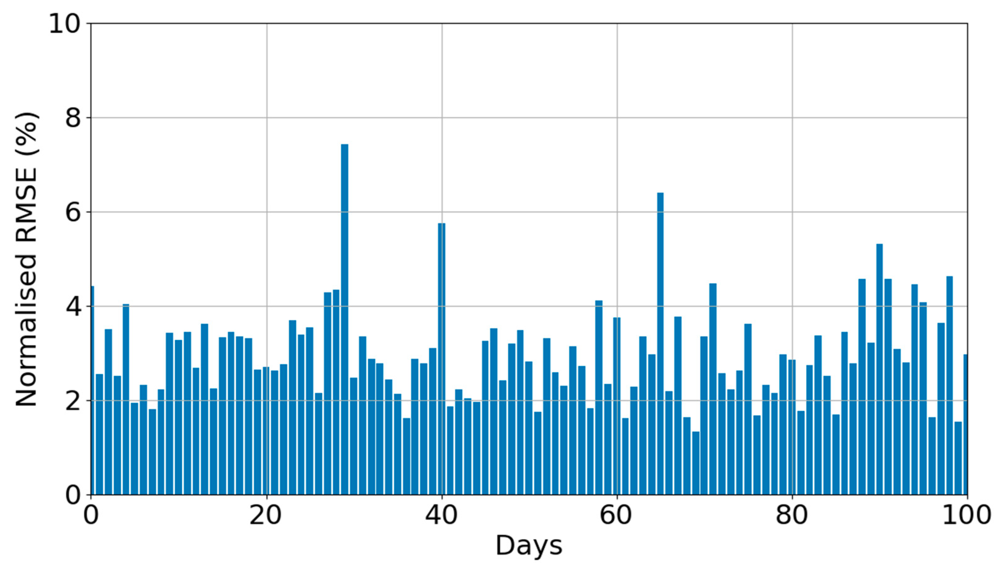
Figure 3 shows the daily nRMSE of the model when trained using 70% of the available data points and evaluated on the test set. Overall, the XGBoost predictive model yielded an average nRMSE of 2.99% over the test set period, while the daily nRMSE predictions were lower than 5% (except for three days), demonstrating high accuracies at varying irradiance level conditions.
In case of field data unavailability, the 1-year synthetic generated time series of the test-bench PV system was used for the training procedure and development of the XGBoost model. For a 70:30% train and test set approach, the machine learning model yielded a nRMSE value of 5.22%, while for a 10:30% train and test set approach, the nRMSE was 5.75%. It is worth noting here that the test set was the same as above (30% of the actual PV dataset containing the field measurements).
3.3. Failure Detection Algorithm (FDA) Classification Performance
The capability of the proposed XGBoost classifier to distinguish normal from fault data points was assessed against the imputed fault conditions with 5% power loss. The classifier was developed by using either synthetically generated or actual performance data for the train set. The results of this analysis, summarized in
Table 5, showed that the classifier (with oversampling) was capable of diagnosing fault conditions at accuracies of 84.50% and 85.40% when trained with synthetic or actual performance data with fault patterns, respectively. The classifier trained with synthetic data presented high sensitivity and specificity indicators of 82.55% and 86.70%, respectively. These indicators were in close agreement with the results obtained when training the classifier against actual performance data from the test-bench system (sensitivity of 83.91% and specificity of 87.03%), providing evidence that accurate classification models can be constructed by utilizing synthetic datasets and emulated fault patterns.
Finally, the performance accuracy of the classifier for fault diagnosis was improved when oversampling the train set. For example, when the classifier was trained using field data, accuracies of 85.40% and 82.05% and sensitivities of 83.91% and 76.55% were obtained for the dataset with and without oversampling, respectively.
For comparative purposes, the diagnostic ability of the XGBoost classifier constructed with synthetic data was compared against a statistical anomaly detector. More specifically, the S-H-ESD algorithm was applied on the reduced power time series data to detect data anomalies (indicating fault conditions). The performance of the S-H-ESD algorithm for diagnosing 5% power reducing incidents was evaluated using a binary confusion metric. The fault detection results from the S-H-ESD application are summarized in
Table 6. The anomaly detection algorithm could diagnose fault conditions causing 5% power loss (detected either as global or local anomalies), achieving an accuracy of 76.25%, a sensitivity of 76.22%, and a specificity of 76.28%.
The obtained results demonstrated that the XGBoost classifier outperformed the statistical S-H-ESD algorithm for PV fault diagnosis. However, it is worth noting that for the S-H-ESD application there is no need for training data.
The XGBoost algorithm was then used for detecting “real” faults. The optimum XGBoost classifier was used to classify a labeled test set containing 4465 data points (4420 and 45 normal and fault data points, respectively). The fault data points were attributed to five types of failures (open- and short-circuited PV module, inverter shutdown, shorted bypass diode, and partial shading) that were emulated at the test-bench PV system. The fault classification results using field-emulated measurements are summarized in
Table 7. A 30:30% sequential train and test set approach was selected to illustrate low data training partitions. The classifier presented high sensitivity (99.98%) and specificity (84.62%), indicating its suitability for diagnosing different common failure types in operating PV systems. Once the failures are detected, O&M teams can perform corrective actions to minimize the power loss and hence increase revenue.
4. Discussion
In this work, a health-state architecture for PV system monitoring and failure diagnosis was presented. Within this framework, the performed analysis revealed useful information for the construction of accurate predictive and classification models for sites that either lack in amounts or quality of historic data. Throughout this analysis, the following findings were obtained:
The DQRs form a fundamental stage of the proposed health-state architecture. The data quality methodology can be applied on raw field measurements for a preliminary distinction between normal and erroneous data or fault condition events, prior to predictive model’s development procedure.
The XGBoost machine learning model can be used for both PV system power prediction (regression model) and failure diagnosis (classification model).
Regarding the regression model, the most significant input features were the
,
,
, and
. This finding is aligned with that of [
29], where the same input parameters were derived as the highly correlated features for the development of an optimal artificial neural network (ANN) predictive model for power production forecasting.
The XGBoost regression model exhibited the lowest average nRMSE of 2.99% when trained with 70% field data partition share. Even at low data training partitions (i.e., 10% of the entire dataset), the predictive model yielded an average nRMSE of 3.40%. In relation to previous literature, authors in [
38] developed a model for on-line monitoring and fault detection in large-scale PV installations (of 1 MW
p) with reported nRMSE values ranging from 10.51% to 16.71% when using inverter measurements. Similarly, power predictions at the inverter level (approximately 350 kW
p) in [
39] reported nRMSE values in the range of 9.68% to 19.47%. Finally, lower nRMSE values (e.g., 1.44%) have also been reported in the literature for predicting the DC power of small-scale PV systems (1.2 kW
p) [
18]. However, the validation process in [
18] was conducted against performance under normal operating conditions using laboratory-scale data, which differentiates it from our study. In this work, the model’s prediction performance was assessed using the test set that included both normal and fault conditions, resulting in higher nRMSE.
With respect to the XGBoost classifier, the results showed high fault diagnostic capabilities, achieving a specificity of 87.03%, accuracy of 85.40%, and a sensitivity of 83.91% when using on-site data for the training procedure. Similarly, with the use of synthetic data, the classifier presented high sensitivity and specificity indicators of 82.54% and 86.70%, respectively. Fault detection accuracies ranging from 93.09% up to ~99% have been reported in the literature [
40,
41]. In particular, a monitoring system for online fault diagnosis (tested on a 5 kW
p PV system) demonstrated a detection accuracy of 93.09%, while the accuracy of the classification stage was 95.44% [
40]. Likewise, a support vector machine (SVM) achieved up to 94.74% accuracy for detecting short-circuit conditions [
41]. The SVM model was trained with simulated data and tested in a small-scale PV system. Similarly, a fuzzy logic system for fault diagnosis was presented in [
42] and demonstrated detection accuracies ranging from 95.27% to 98.8% for a 1.1 kW
p and 0.52 kW
p PV systems. Finally, a fault detection algorithm based on ANN was developed to detect PV module disconnections [
43]. The benchmarking results from a 2.2 kW
p and 4.16 kW
p PV systems provided up to 98.1% accuracy for partial shading and PV module disconnection faults. Despite the relatively high performance of the reported algorithms and systems, the investigated faults cause relative power reduction from 10% to 100%. In this work, fault events that may even cause small power loss (i.e., 5% relative power reduction) were investigated, thus justifying the lower detection accuracy provided by the XGBoost classifier.
Improved performance accuracy and sensitivity was obtained by the classifier when oversampling the training data. When the classifier was trained using field data, accuracies of 85.40% and 82.05% and sensitivities of 83.91% and 76.55% were obtained for the dataset with and without oversampling, respectively.
The machine learning classifier for PV failure diagnosis outperformed the S-H-ESD statistical anomaly detection technique, which achieved an accuracy of 76.25%, a sensitivity of 76.22%, and a specificity of 76.28%. However, it is worth noting the value of the S-H-ESD statistical technique, as it does not require any training.
The XGBoost classifier proved capable of detecting field-emulated failures in the test-bench PV system, achieving high sensitivity and specificity indicators (99.98% and 84.62%, respectively). The XGBoost classifier outperformed other machine learning classifiers (such as decision trees, k-nearest neighbors, support vector machine, and fuzzy inference systems) reported in a previous study [
27] that had been developed to classify the field-emulated failure signatures of open- and short-circuited PV module, inverter shutdown, shorted bypass diode, and partial shading in the test-bench PV system.
Overall, this study addresses the current research challenge in bringing unified approaches for robust and scalable PV system health-state monitors. The obtained results demonstrated that an accurate architecture for PV performance prediction and fault detection can be constructed with minimal input features by utilizing either low amounts of on-site historic data or entirely synthetically generated data and fault patterns. The proposed health-state architecture presents some advantages compared to other existing ones reported in the literature, which can be summarized as follows:
It allows real-time fault detection of incidents that may even cause small power loss (i.e., 5% relative power reduction), ensuring optimal PV plant operation;
A combined regression and classification XGBoost model was used to predict power output and detect typical power-related faults;
The XGBoost model proved to be accurate for PV system performance prediction and fault detection, even when trained using synthetic generated data;
It can be constructed regardless of historic data availability and quality.
The analytical architecture can be integrated into existing/new PV monitoring systems, thus leading to performance improvements and, in return, minimizing both energy and economic losses. However, it lacks extensive benchmarking on multiple PV system topologies and locations, which will be the focus of future work. Finally, future research should focus on developing a fault diagnostic technique that offers a reduced false alarm rate (i.e., the number of FP) [
7].
5. Conclusions
A health-state architecture for advanced PV system monitoring and fault diagnosis was presented in this paper. The proposed architecture incorporates DQRs for effective field data preparation and a machine learning model (i.e., the XGBoost), which was used for both PV power prediction (regression model) and detection of typical power-related faults (classifier model).
The XGBoost predictive model was developed and evaluated using field data from a test-bench PV system installed in Cyprus, achieving low prediction errors. The prediction model was optimally trained on low fractions of on-site data and minimal features to postulate its accuracy with reduced dependency of site data. Concurrently, the developed XGBoost classifier was trained under an enhanced supervised learning regime and proved to be effective for PV fault diagnosis, even when trained using synthetic data.
Overall, the results provided proof that robust health-state architectures can be built using synthetic data and fault patterns backed on low amounts of on-site historic data. The developed data-driven algorithms can form integral parts of monitoring systems for real-time and uninterrupted monitoring of PV plants. Furthermore, this work provided useful insights on how to construct accurate predictive and classification models for the timely and reliable detection of faults in PV systems. Such health-state architectures for PV plants can have positive implications in field O&M operations (e.g., mitigation actions) and costs. By providing information and detecting underperformance incidents in PV systems, PV plant owners, operators, and managers can perform corrective actions, thus minimizing energy production losses and maximizing revenue.
While the accuracies of the proposed regressor and classifier are high, there is still room for improvement. Future work will focus on the development of more robust, accurate, and scalable PV health-state architectures tested on multiple PV system topologies and locations to verify the installation- and location-independence of the health-state monitor for PV monitoring and fault diagnosis.
Author Contributions
Conceptualization, A.L. and G.M.; methodology, A.L., G.P., M.T., J.L.-L. and G.M.; software, A.L., G.P. and G.M.; validation, A.L., M.T., J.L.-L. and G.M.; formal analysis, A.L., G.P., M.T. and G.M.; writing—original draft preparation, A.L. and M.T.; writing—review and editing, A.L., M.T., J.L.-L., G.M. and G.E.G.; visualization, A.L. and G.P.; supervision, G.E.G.; project administration, G.E.G.; funding acquisition, G.E.G. All authors have read and agreed to the published version of the manuscript.
Funding
This research was funded by the 1C4PV SOLAR-ERA.NET project and the Research and Innovation Foundation (RIF) of Cyprus (RIF project number: P2P/SOLAR/0818/0010) for the UCY authors. The work of M. Theristis was supported by the U.S. Department of Energy’s Office of Energy Efficiency and Renewable Energy (EERE) under the Solar Energy Technologies Office Award Number 38267.
Institutional Review Board Statement
Not applicable.
Informed Consent Statement
Not applicable.
Data Availability Statement
Restrictions apply to the availability of the test PV plant data. Data was obtained from the University of Cyprus and are only available on request from the university. The data are not publicly available due to privacy reasons.
Acknowledgments
The work of UCY authors was supported by the 1C4PV project. Project 1C4PV is supported under the umbrella of SOLAR-ERA.NET Cofund by the Centro para el Desarrollo Tecnológico Industrial (CDTI), the Scientific and Technological Research Council of Turkey and the Research and Innovation Foundation (RIF) of Cyprus. SOLAR-ERA.NET is supported by the European Commission within the EU Framework Programme for Research and Innovation HORIZON 2020 (Cofund ERA-NET Action, N° 691664). The work of M. Theristis was supported by the U.S. Department of Energy’s Office of Energy Efficiency and Renewable Energy (EERE) under the Solar Energy Technologies Office Award Number 38267. Sandia National Laboratories is a multimission laboratory managed and operated by National Technology & Engineering Solutions of Sandia, LLC, a wholly owned subsidiary of Honeywell International Inc., for the U.S. Department of Energy’s National Nuclear Security Administration under contract DE-NA0003525. This article describes objective technical results and analysis. Any subjective views or opinions that might be expressed in this article do not necessarily represent the views of the U.S. Department of Energy or the Unites States Government.
Conflicts of Interest
The authors declare no conflict of interest.
Abbreviations
The following abbreviations were used in this manuscript:
| SMOTE | Synthetic Minority Oversampling Technique |
| c-Si | crystalline-Silicon |
| DAQ | data acquisition |
| DQRs | Data Quality Routines |
| XGBoost | eXtream Gradient Boosting |
| FDA | Failure Detection Algorithm |
| FDRs | Failure Diagnosis Routines |
| LCOE | levelized cost of electricity |
| MIT | minimum irradiance threshold |
| nRMSE | normalized root mean square error |
| PR | performance ratio |
| PV | photovoltaic |
| RMSE | root mean squared error |
| SAPM | Sandia PV Array Performance Model |
| S-H-ESD | Seasonal Hybrid Extreme Studentized Deviates |
| TL | threshold level |
| AC output power |
| Ambient temperature |
| Array DC current |
| Module temperature |
| Array DC power |
| Wind direction |
| Downtimes |
| Solar elevation |
| In-plane irradiance |
| Array energy yield |
| Final PV system yield |
| Reference yield |
| Solar azimuth |
| Useful periods of time |
| Array DC Voltage |
| Wind speed |
References
- Livera, A.; Theristis, M.; Makrides, G.; Georghiou, G.E. Recent advances in failure diagnosis techniques based on performance data analysis for grid-connected photovoltaic systems. Renew. Energy 2019, 133, 126–143. [Google Scholar] [CrossRef]
- Livera, A.; Theristis, M.; Koumpli, E.; Theocharides, S.; Makrides, G.; Sutterlueti, J.; Stein, J.S.; Georghiou, G.E. Data processing and quality verification for improved photovoltaic performance and reliability analytics. Prog. Photovoltaics Res. Appl. 2021, 29, 143–158. [Google Scholar] [CrossRef]
- Woyte, A.; Richter, M.; Moser, D.; Mau, S.; Reich, N.; Jahn, U. Monitoring of photovoltaic systems: Good practices and systematic analysis. In Proceedings of the 28th European Photovoltaic Solar Energy Conference and Exhibition (EU PVSEC), Paris, France, 4 October 2013; pp. 3686–3694. [Google Scholar]
- Manzano, S.; Guevara, D.; Rios, A. An Overview of Remote Monitoring Pv Systems: Acquisition, Storages, Processing and Publication of Real-Time Data Based on Cloud Computing. In Proceedings of the 13th International Workshop on Large-Scale Integration of Wind Power into Power Systems as well as on Transmission Networks for Offshore Wind Power Plants & 4th Solar Integration Workshop, Berlin, Germany, 11–13 November 2014. [Google Scholar]
- Samara, S.; Natsheh, E. Intelligent Real-Time Photovoltaic Panel Monitoring System Using Artificial Neural Networks. IEEE Access 2019, 7, 50287–50299. [Google Scholar] [CrossRef]
- Drews, A.; de Keizer, A.C.; Beyer, H.G.; Lorenz, E.; Betcke, J.; van Sark, W.G.J.H.M.; Heydenreich, W.; Wiemken, E.; Stettler, S.; Toggweiler, P.; et al. Monitoring and remote failure detection of grid-connected PV systems based on satellite observations. Sol. Energy 2007, 81, 548–564. [Google Scholar] [CrossRef] [Green Version]
- Fazai, R.; Abodayeh, K.; Mansouri, M.; Trabelsi, M.; Nounou, H.; Nounou, M.; Georghiou, G.E. Machine learning-based statistical testing hypothesis for fault detection in photovoltaic systems. Sol. Energy 2019, 190, 405–413. [Google Scholar] [CrossRef]
- Platon, R.; Martel, J.; Woodruff, N.; Chau, T.Y. Online Fault Detection in PV Systems. IEEE Trans. Sustain. Energy 2015, 6, 1200–1207. [Google Scholar] [CrossRef]
- Woyte, A.; Richter, M.; Moser, D.; Green, M.; Mau, S.; Beyer, H.G. Analytical Monitoring of Grid-Connected Photovoltaic Systems: Good Practice for Monitoring and Performance Analysis; IEA PVPS Task 13, Subtask 2; Report IEA-PVPS T13-03: 2014; International Energy Agency: Paris, France, March 2014. [Google Scholar]
- Dhibi, K.; Fezai, R.; Mansouri, M.; Trabelsi, M.; Kouadri, A.; Bouzara, K.; Nounou, H.; Nounou, M. Reduced Kernel Random Forest Technique for Fault Detection and Classification in Grid-Tied PV Systems. IEEE J. Photovolt. 2020, 10, 1864–1871. [Google Scholar] [CrossRef]
- Garoudja, E.; Harrou, F.; Sun, Y.; Kara, K.; Chouder, A.; Silvestre, S. Statistical fault detection in photovoltaic systems. Sol. Energy 2017, 150, 485–499. [Google Scholar] [CrossRef]
- Jones, C.B.; Stein, J.S.; Gonzalez, S.; King, B.H. Photovoltaic system fault detection and diagnostics using Laterally Primed Adaptive Resonance Theory neural network. In Proceedings of the 42nd IEEE Photovoltaic Specialist Conference (PVSC), New Orleans, LA, USA, 14–19 June 2015. [Google Scholar] [CrossRef]
- Livera, A.; Theristis, M.; Stein, J.S.; Georghiou, G.E. Failure Diagnosis and Trend-Based Performance Losses Routines for the Detection and Classification of Incidents in Large-Scale Photovoltaic Systems. In Proceedings of the 38h European Photovoltaic Solar Energy Conference (EU PVSEC), Lisbon, Portugal, 6–10 September 2021; pp. 973–978. [Google Scholar]
- Zhao, Y.; Balboni, F.; Arnaud, T.; Mosesian, J.; Ball, R.; Lehman, B. Fault experiments in a commercial-scale PV laboratory and fault detection using local outlier factor. In Proceedings of the 40th IEEE Photovoltaic Specialist Conference (PVSC), Denver, CO, USA, 8–13 June 2014. [Google Scholar] [CrossRef]
- Chouder, A.; Silvestre, S. Automatic supervision and fault detection of PV systems based on power losses analysis. Energy Convers. Manag. 2010, 51, 1929–1937. [Google Scholar] [CrossRef]
- Ding, H.; Ding, K.; Zhang, J.; Wang, Y.; Gao, L.; Li, Y.; Chen, F.; Shao, Z.; Lai, W. Local outlier factor-based fault detection and evaluation of photovoltaic system. Sol. Energy 2018, 164, 139–148. [Google Scholar] [CrossRef]
- Belaout, A.; Krim, F.; Mellit, A.; Talbi, B.; Arabi, A. Multiclass adaptive neuro-fuzzy classifier and feature selection techniques for photovoltaic array fault detection and classification. Renew. Energy 2018, 127, 548–558. [Google Scholar] [CrossRef]
- Livera, A.; Theristis, M.; Makrides, G.; Ransome, S.; Sutterlueti, J.; Georghiou, G.E. Optimal development of location and technology independent machine learning photovoltaic performance predictive models. In Proceedings of the 46th IEEE Photovoltaic Specialist Conference (PVSC), Chicago, IL, USA, 16–21 June 2019; pp. 1270–1275. [Google Scholar]
- Ascencio-Vásquez, J.; Brecl, K.; Topič, M. Methodology of Köppen-Geiger-Photovoltaic climate classification and implications to worldwide mapping of PV system performance. Sol. Energy 2019, 191, 672–685. [Google Scholar] [CrossRef]
- Phinikarides, A.; Makrides, G.; Zinsser, B.; Schubert, M.; Georghiou, G.E. Analysis of photovoltaic system performance time series: Seasonality and performance loss. Renew. Energy 2015, 77, 51–63. [Google Scholar] [CrossRef]
- International Electrotechnical Commission. Photovoltaic System Performance—Part 1: Monitoring; IEC 61724-1:2017; IEC: Geneva, Switzerland, 2017. [Google Scholar]
- Theristis, M.; Venizelou, V.; Makrides, G.; Georghiou, G.E. Chapter II-1-B—Energy yield in photovoltaic systems. In McEvoy’s Handbook of Photovoltaics, third ed; Kalogirou, S.A., Ed.; Academic Press: Cambridge, MA, USA, 2018; pp. 671–713. ISBN 9780128099216. [Google Scholar]
- Reda, I.; Andreas, A. Solar Position Algorithm for Solar Radiation Applications; National Renewable Energy Laboratory Technical Report; NREL/Tp-560-34302; National Renewable Energy Laboratory: Golden, CO, USA, 2008. [Google Scholar] [CrossRef] [Green Version]
- King, D.L.; Boyson, W.E.; Kratochvil, J.A. Photovoltaic Array Performance Model; SANDIA Report SAND2004-3535; Sandia National Laboratories: Albuquerque, NM, USA, 2004; Volume 8. [Google Scholar]
- Holmgren, W.F.; Hansen, C.W.; Mikofski, M.A. Pvlib Python: A Python Package for Modeling Solar Energy Systems. J. Open Source Softw. 2018, 3, 884. [Google Scholar] [CrossRef] [Green Version]
- Köntges, M.; Kurtz, S.; Packard, C.; Jahn, U.; Berger, K.A.; Kato, K.; Friesen, T.; Liu, H.; Van Iseghem, M. Performance and reliability of photovoltaic systems, Subtask 3.2: Review of Failures of Photovoltaic Modules; Report IEA-PVPS T13-01: 2014; IEA International Energy Agency: Paris, France, 2014. [Google Scholar]
- Livera, A.; Theristis, M.; Makrides, G.; Sutterlueti, J.; Georghiou, G.E. Advanced diagnostic approach of failures for grid-connected photovoltaic (PV) systems. In Proceedings of the 35th European Photovoltaic Solar Energy Conference (EU PVSEC), Brussels, Belgium, 24–27 September 2018; pp. 1548–1553. [Google Scholar]
- Chen, T.; Guestrin, C. XGBoost: A Scalable Tree Boosting System. In Proceedings of the KDD’16: Proceedings of the 22nd ACM SIGKDD International Conference on Knowledge Discovery and Data Mining, San Francisco, CA, USA, 13–17 August 2016. [Google Scholar]
- Theocharides, S.; Makrides, G.; Livera, A.; Theristis, M.; Kaimakis, P.; Georghiou, G.E. Day-ahead photovoltaic power production forecasting methodology based on machine learning and statistical post-processing. Appl. Energy 2020, 268, 115023. [Google Scholar] [CrossRef]
- Han, H.; Wang, W.Y.; Mao, B.H. Borderline-SMOTE: A New Over-Sampling Method in Imbalanced Data Sets Learning. In Proceedings of the International Conference on Intelligent Computing, Hefei, China, 23–26 August 2005; Volume 3644, pp. 878–887. [Google Scholar] [CrossRef]
- Rosner, B. On the detection of many outliers. Technometrics 1975, 17, 221–227. [Google Scholar] [CrossRef]
- Rosner, B. Percentage points for a Generalized ESD many-outlier procedure. Technometrics 1983, 25, 165–172. [Google Scholar] [CrossRef]
- Twitter AnomalyDetection R Package; GitHub: San Francisco, CA, USA, 2015.
- Theocharides, S.; Makrides, G.; Kyprianou, A.; Georghiou, G.E. Machine Learning Algorithms for Photovoltaic System Power Output Prediction. In Proceedings of the 5th IEEE International Energy Conference (ENERGYCON), Limassol, Cyprus, 3–7 June 2018; pp. 1–6. [Google Scholar] [CrossRef]
- Lantz, B. Machine Learning with R; Packt Publishing Ltd.: Birmingham, UK, 2013; ISBN 9789811068089. [Google Scholar]
- Jufri, F.H.; Oh, S.; Jung, J. Development of Photovoltaic abnormal condition detection system using combined regression and Support Vector Machine. Energy 2019, 176, 457–467. [Google Scholar] [CrossRef]
- Theristis, M.; Livera, A.; Jones, C.B.; Makrides, G.; Georghiou, G.E.; Stein, J.S. Nonlinear Photovoltaic Degradation Rates: Modeling and Comparison Against Conventional Methods. IEEE J. Photovolt. 2020, 10, 1112–1118. [Google Scholar] [CrossRef]
- Ventura, C.; Tina, G.M. Utility scale photovoltaic plant indices and models for on-line monitoring and fault detection purposes. Electr. Power Syst. Res. 2016, 136, 43–56. [Google Scholar] [CrossRef]
- Ventura, C.; Tina, G.M. Development of models for on-line diagnostic and energy assessment analysis of PV power plants: The study case of 1 MW Sicilian PV plant. Energy Procedia 2015, 83, 248–257. [Google Scholar] [CrossRef] [Green Version]
- Lazzaretti, A.E.; da Costa, C.H.; Rodrigues, M.P.; Yamada, G.D.; Lexinoski, G.; Moritz, G.L.; Oroski, E.; de Goes, R.E.; Linhares, R.R.; Stadzisz, P.C.; et al. A monitoring system for online fault detection and classification in photovoltaic plants. Sensors 2020, 20, 4688. [Google Scholar] [CrossRef] [PubMed]
- Yi, Z.; Etemadi, A.H. Line-to-line fault detection for photovoltaic arrays based on multi-resolution signal decomposition and two-stage support vector machine. IEEE Trans. Ind. Electron. 2017, 64, 8546–8556. [Google Scholar] [CrossRef]
- Dhimish, M.; Holmes, V.; Mehrdadi, B.; Dales, M. Diagnostic method for photovoltaic systems based on six layer detection algorithm. Electr. Power Syst. Res. 2017, 151, 26–39. [Google Scholar] [CrossRef]
- Hussain, M.; Dhimish, M.; Titarenko, S.; Mather, P. Artificial neural network based photovoltaic fault detection algorithm integrating two bi-directional input parameters. Renew. Energy 2020, 155, 1272–1292. [Google Scholar] [CrossRef]
| Publisher’s Note: MDPI stays neutral with regard to jurisdictional claims in published maps and institutional affiliations. |
© 2022 by the authors. Licensee MDPI, Basel, Switzerland. This article is an open access article distributed under the terms and conditions of the Creative Commons Attribution (CC BY) license (https://creativecommons.org/licenses/by/4.0/).


 ,
, 


