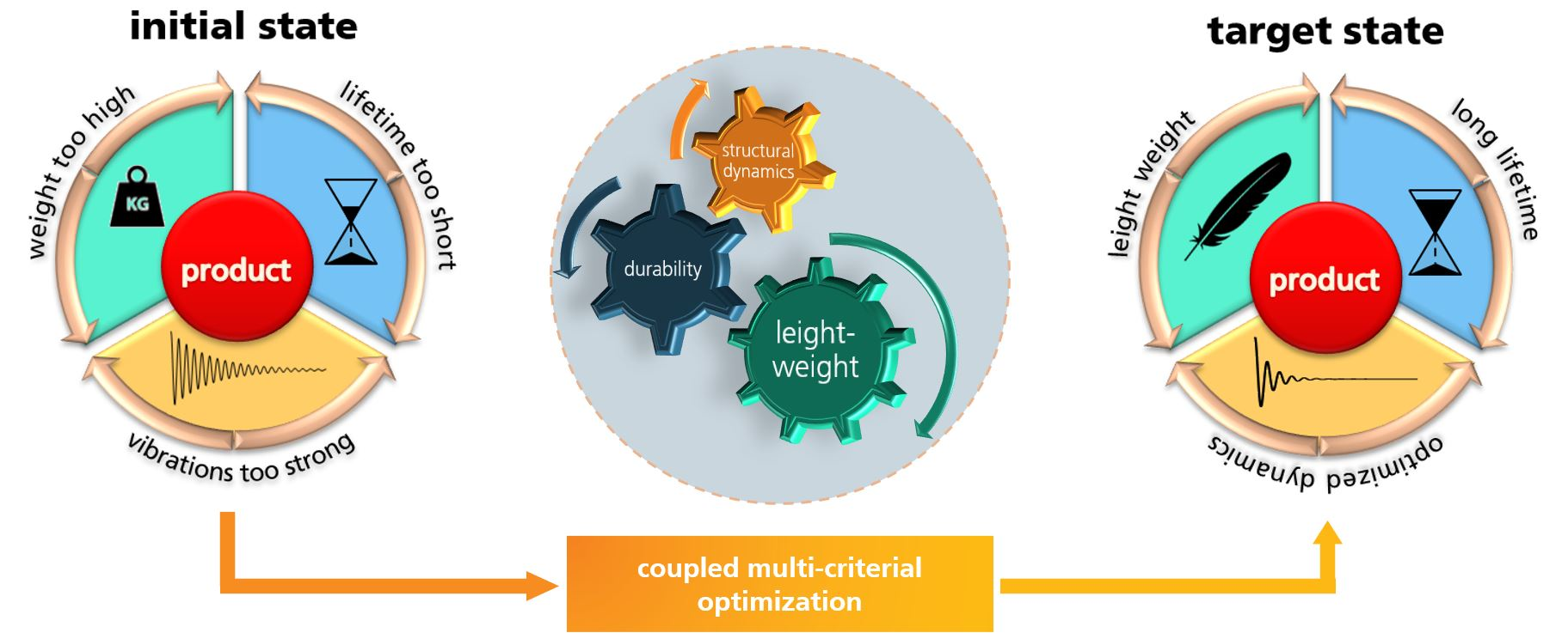
The overall goal of the optimization process is to find a set of parameters that minimizes both the dynamic amplitudes and the damage values of the critical welds with a minimum expense of additional mass. Since these demands are in conflict with each other and cannot be minimized at the same time, the optimization problem can be seen as a MDO task from a mathematical point of view, which can be denoted as a multi-criterial optimization since several criteria are considered. However, to gain a good understanding of the problem, the system is initially analysed in the three dimensions structural dynamics, durability and lightweight design independently.
3.1.1. Mono-Criterial Optimization
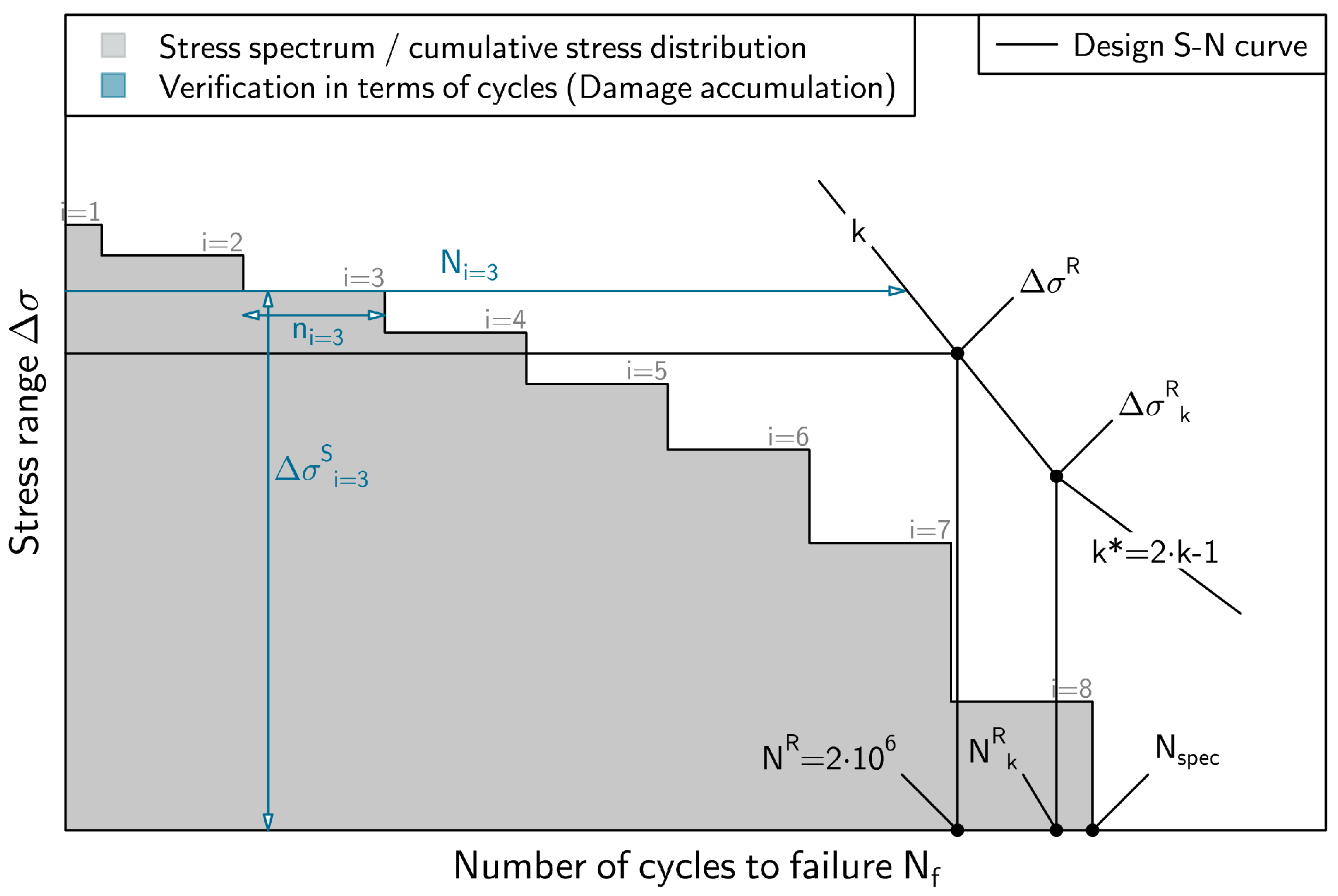
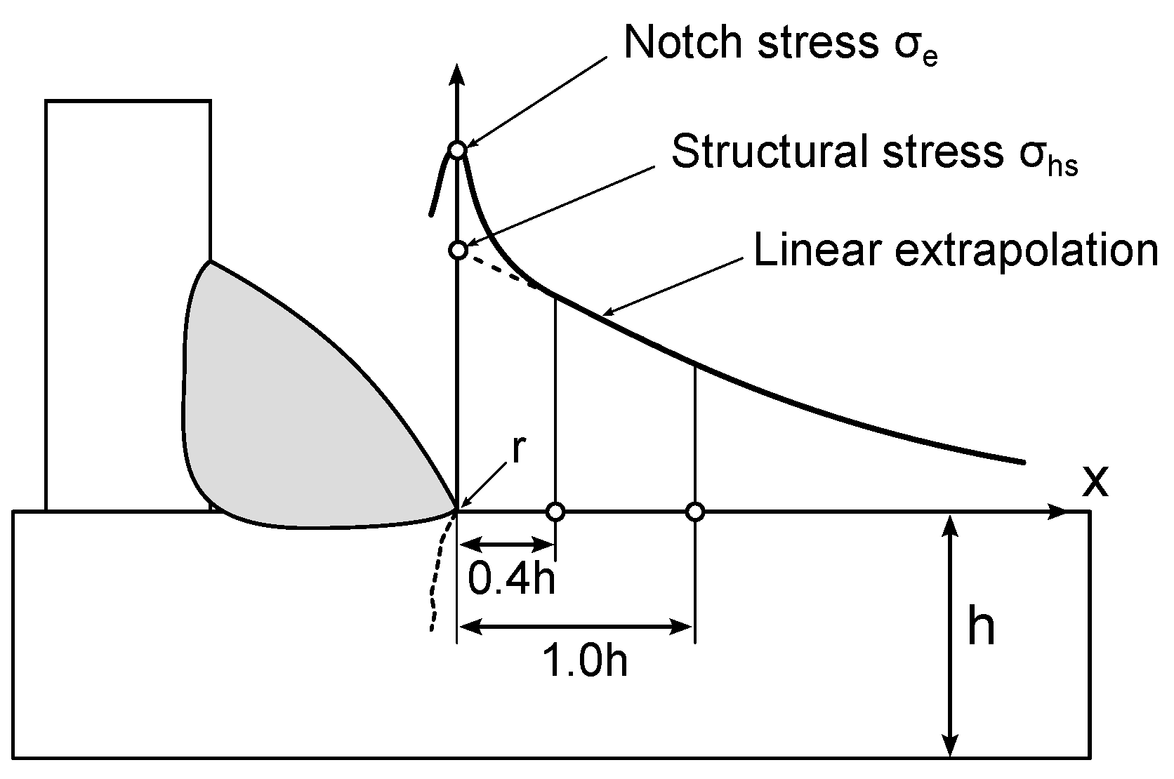
Input for the damage accumulation are the counted hot-spot stress ranges using ASTM 1049-85 based on the simulated stress-time course and the design S–N curve with = 100 MPa and the slopes and . The damage D is evaluated with the linear damage accumulation.
Four values are defined to asses each parameter set:
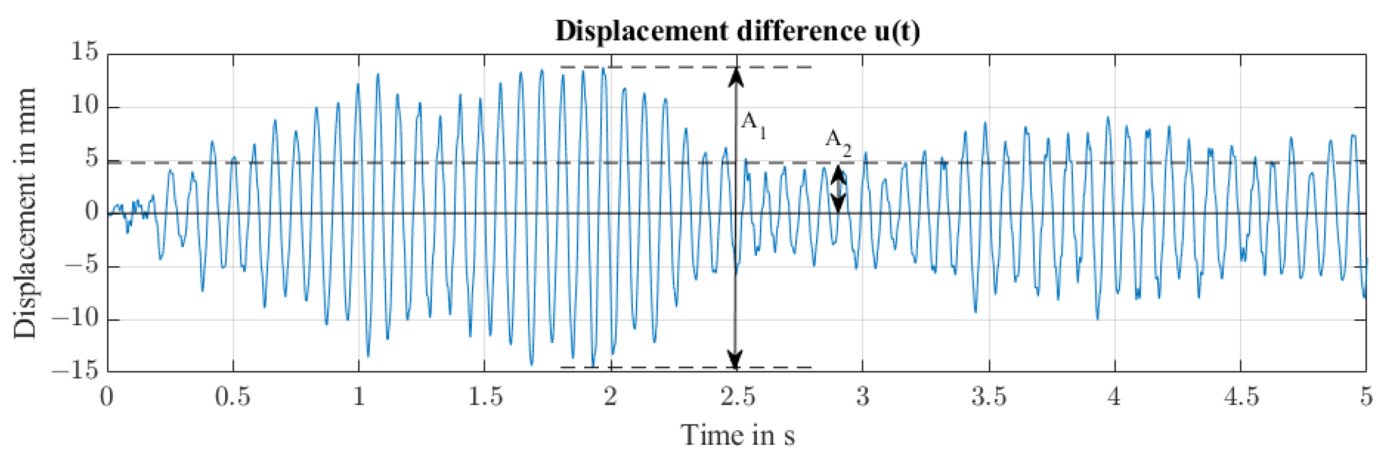
is the maximum displacement range (peak to peak) at the outer tip within the given time frame,
is the mean displacement at the same point,
M is the overall mass and
D is the damage value of the most critical weld, that is the maximum of all damage values
. The equations for each value is given in (
22) to (
25) with
u denoting the difference in displacement in
z-direction (Equation (
26)).
The calculation of
and
according to Equations (
22) and (
23) is visualized in
Figure 8 for exemplary time data of
u and a simulation time of 5 s.
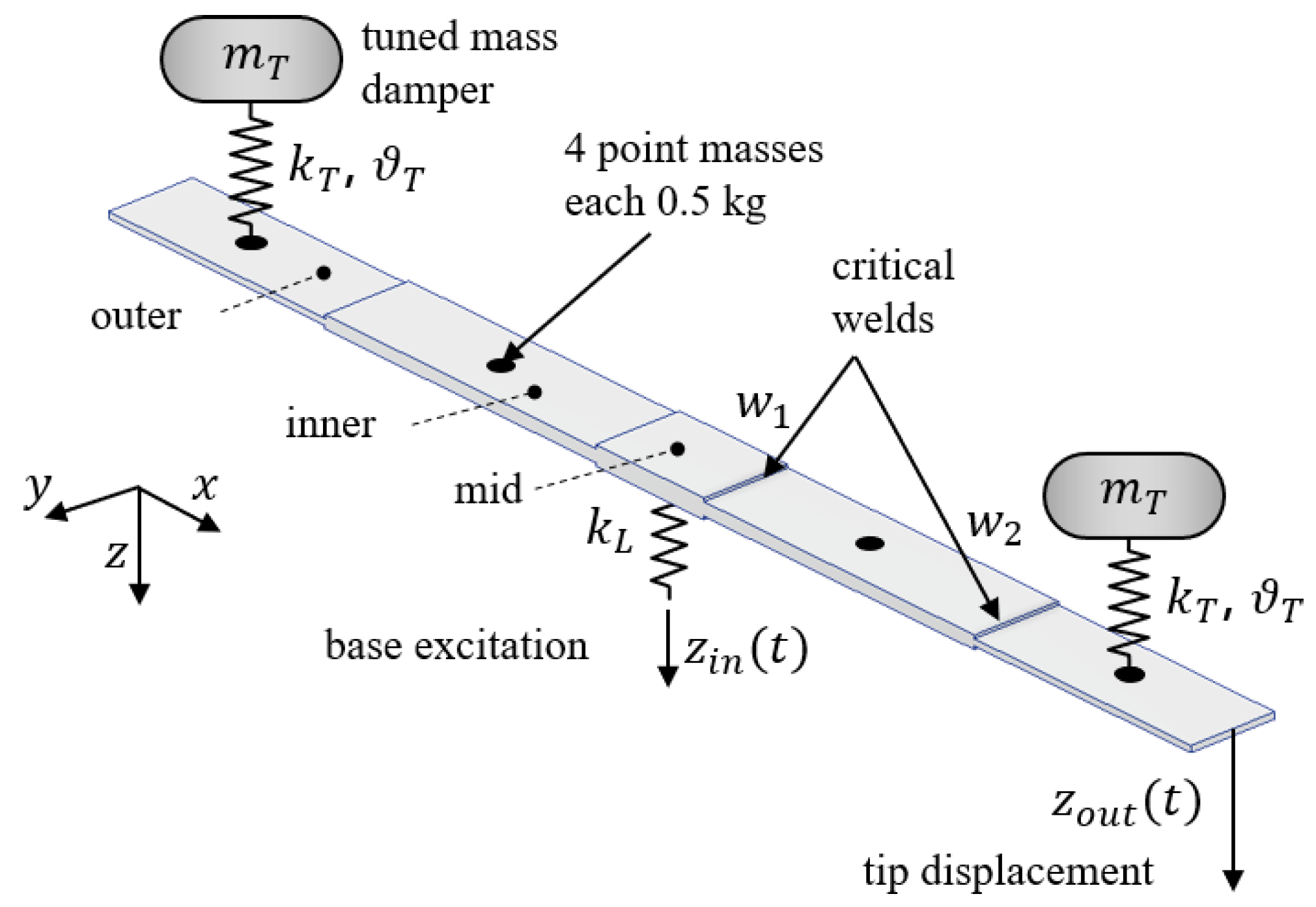
Since each value should be as low as possible, various optimization algorithms can be used to find optimal design parameters in a given design space. However, for a simple structure as this a full factorial parameter variation can be performed with reasonable computational effort. This typically gives a good understanding of the problem and allows an illustrative 2D visualization in the case of only two design variables. Therefore, the simulation model was run 21 × 21 = 441 times, while the absorber mass was varied from 0 to 0.300 kg in steps of 0.015 kg and the absorber stiffness was varied from 100 N/m to 900 N/m in steps of 40 N/m. The damping ratio was kept constant at 3%, which is a realistic average value for vibration absorbers with elastomer-based damping.
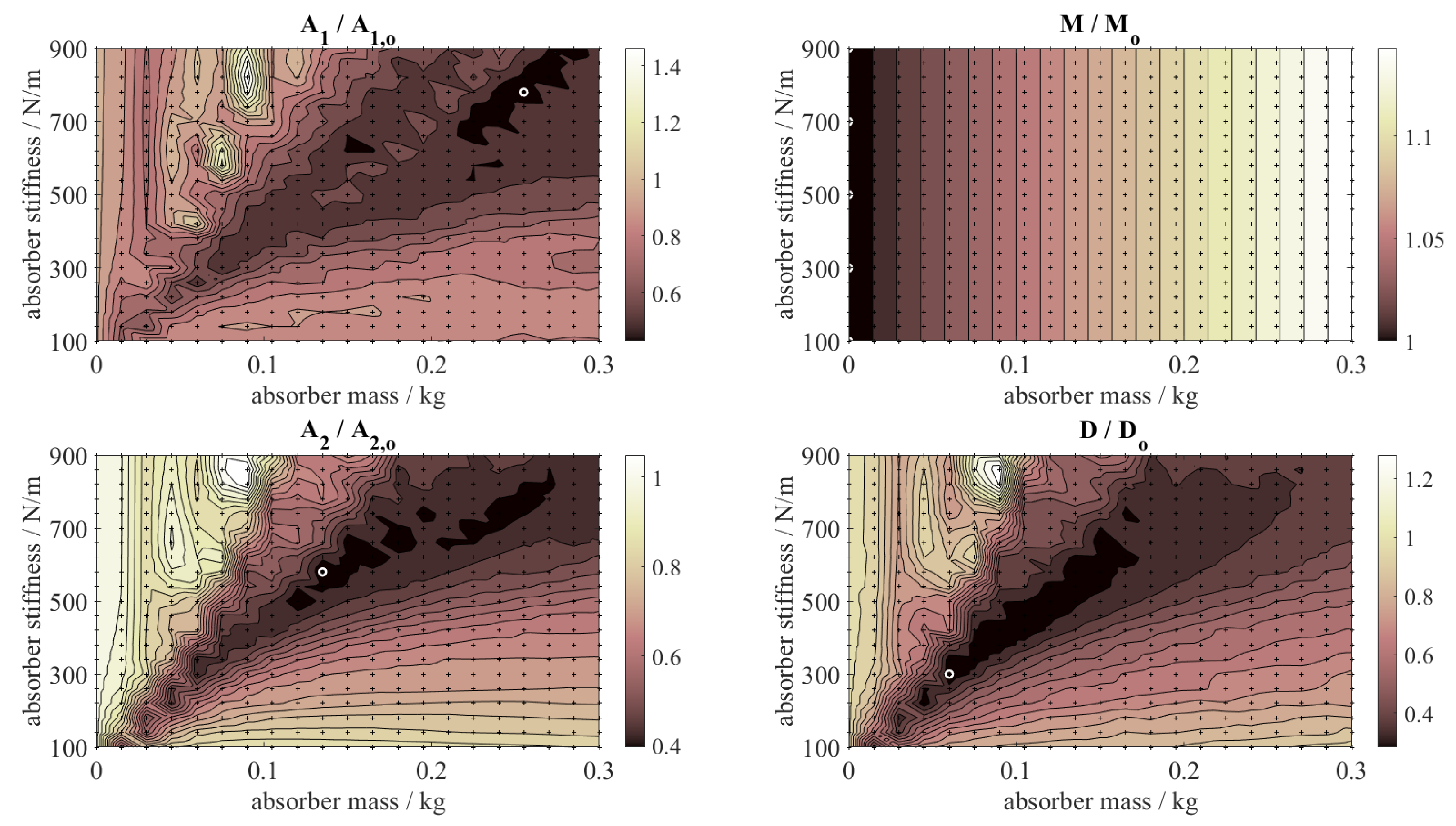
Figure 9 shows the relative values for
,
,
M, and
D for the full factorial parameter variation (relative to the corresponding values of the initial system, denoted as
,
,
, and
). The optimal value is marked in each case and given in
Table 3, together with the corresponding design parameters mass
, stiffness
, and the related undamped eigenfrequency of the absorber
.
As observed, the single parameter optimization leads to very different optimal design parameters. The value can be reduced most effectively with an absorber mass of 0.255 kg tuned to 8.85 Hz, while the mean displacement is lowest for an absorber mass of 0.135 kg tuned to 10.5 Hz. The best lightweight design has no absorber at all, and for the most durable design an absorber mass of 0.060 kg tuned to 10.98 Hz is needed. Interestingly, the design parameter set for the best dynamics differs from the one for the best durability, which underlines that evaluating the damage of the structure together with its dynamic behaviour is essential.
With the results shown in
Figure 9 the engineer can choose a proper set of design parameters, taking into account the specific boundary conditions and requirements of the application, and see, at a glance, the implications of a certain design regarding dynamics, durability, and lightweight design.
3.1.2. Multi-Criterial Optimization
For multi-criterial optimization problems in the engineering context many different techniques are known and described in the literature [
33,
34,
35].
Here, the most straight forward approach with weighting functions for each target value and an arithmetic summation of all four components is chosen, which mathematically reduces the problem to the mono-criterial optimization of a cost function. The corresponding equations are given in Equations (
27)–(
30).
For the maximum displacement difference
a step function is chosen to guarantee that a certain threshold value
is never exceeded, which may result from practical considerations in the application ((
27), with
H denoting the Heaviside step function). For the mean displacement
, a quadratic weighting function is chosen with the optimization parameter
. This accounts for the assumption that the vibration of the system should be as low as possible at all times for a good performance (Equation (
28)). For the overall mass
M, a linear weighting function is chosen with the optimization parameter
, assuming that any additional mass is seen as disadvantageous in the application (Equation (
29)). For the damage
D, again a step function is chosen with a threshold value
, taking into account that in many engineering problems a minimum lifetime must be guaranteed, but no further requirements regarding lifetime are made (Equation (
29)). The formulation of these weighting functions and the specification of the parameters can be adjusted to each individual application scenario considering further requirements and boundary conditions of the system.
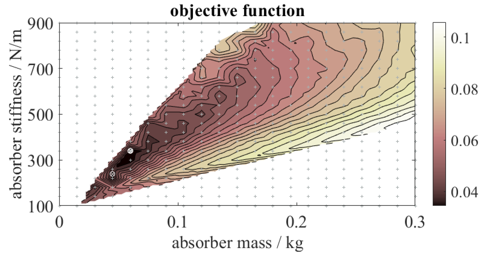
The summation of the weighting functions results in the overall cost function
S (
31) that needs to be minimized.
The optimization parameters for this example are set to
mm,
1/mm²,
1/kg and
= 0.001 as an initial guess. The determination of suitable values is not focused on here as the emphasis is on the methodology. Therefore, the values in this context were chosen exemplary. In practice, engineering expertise, experience, and economic considerations and design restrictions will be used in determining the values. The consideration of individual example cases or a pairwise comparison can also be helpful here. Since full factorial data are available, the goal function
S can easily be visualized and the minimum value identified. The surface plot of
S is shown in
Figure 10. The white areas are invalid regions because the cost function is above 1. The parameters of the minimum are given in the first row of
Table 4.
A standard optimization algorithm is used to find an optimum of
S. In this case, the function fminsearch of Matlab is implemented, which is based on the simplex search method of Lagarias et al. [
36]. Upper and lower limits are additionally implemented and the algorithm was confined to a maximum of 44 evaluations, that is 10% of the number of evaluations of the full factorial simulation. Using the central point of the design space as initial guess (
= 0.150 kg,
= 500 N/m), the algorithm yields a result that is worse compared to the minimum found by the full-factorial search. This is due to the fact that the function
S is not very smooth and the algorithm is susceptible to become caught in local minima. Therefore, the minimum found by the full-factorial search was used as initial guess for another optimization run, yielding now an improved design point. The values of these two optimization runs are given in the second and third row of
Table 4 and
Table 5.
In the optimization runs, the damping ratio has been kept constant at 3%. Finally, an optimization run with the damping ratio as free design variable (within 0.5 and 6%, accounting for practical limitations) is performed, starting from the same design point as before. The results of this optimization process are given in the last row of
Table 4 and
Table 5.
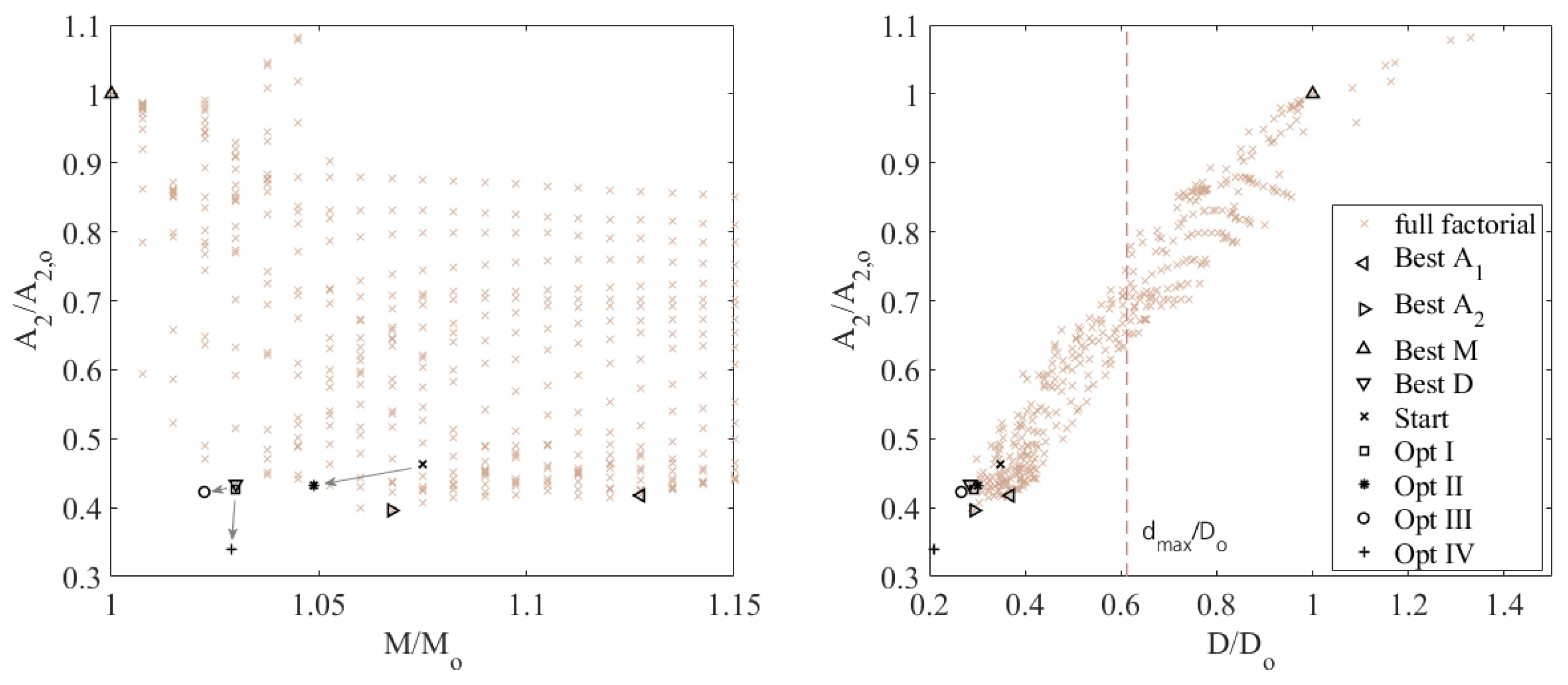
Finally, all optimization results obtained in this study are visualized in
Figure 11 in the three dimensional solution space regarding structural dynamics (in terms of mean displacement
), lightweight design (in terms of overall mass
M) and durability (in terms of damage
D). On the left side, the conflict of goals between overall mass and displacement reduction can be seen. Up to an additional mass of 7% an increasing displacement reduction is possible with higher masses, clearly showing a typical Pareto frontier for these objectives with the optimum found by method I being part of the front line. The Pareto frontier is defined as the sum of all solutions for which any improvement in one objective can only take place if at least one other objective worsens [
37]. The quick optimization run, starting from the centre of the design space (method II), does not reach the Pareto frontier. However, the successive optimization runs starting from the best full factorial value (method III and IV) exceed the Pareto frontier. On the right side, the relationship between displacement reduction and lifetime increase is comprehensible. By and large, a reduction in mean displacement corresponds with the reduction in the damage value; however, this is not true in general as, for some cases, a displacement reduction can also mean a reduction in durability. The dashed line indicates the threshold
.
The results of this simple example show the challenges of multi-criterial optimization. As it can be seen, the full factorial analysis gives a good understanding of the problem and is recommended if the required simulation capacity is available. A pure gradient-based optimization with an arbitrary starting point runs the risk of ending in an unfavourable local minimum due to the complexity of the cost function and should be used with care. A combination of a coarse full-factorial search with a limited number of design parameters and a subsequent gradient-based optimization starting from a previously found minimum can yield satisfactory results with justifiable numerical effort. However, more complex search algorithms that are designed to search for global minima like particle swarm, surrogate, or pattern search are also possible options [
38]. As can be seen, numerical optimization processes need many evaluations and can rapidly become time-consuming for complicated structures in the time domain. In these cases, an evaluation of both the structural dynamics and the durability is recommended in the frequency domain, which is typically accompanied by a loss in accuracy in assessment [
39], but which will lead to better optimization results within a limited computation time.


