Efficient Modal Identification and Optimal Sensor Placement via Dynamic DIC Measurement and Feature-Based Data Compression

Abstract

Full-field non-contact vibration measurements provide a rich dataset for analysing structural dynamics. However, implementing the identification algorithm directly using high-spatial resolution data can be computationally expensive in modal identification. To address this challenge, performing identification in a shape-preserving but lower-dimensional feature space is more feasible. The full-field mode shapes can then be reconstructed from the identified feature mode shapes. This paper discusses two approaches, namely data-dependent and data-independent, for constructing the feature spaces. The applications of these approaches to modal identification on a curved plate are studied, and their performance is compared. In a case study involving a curved plate, it was found that a spatial data compression ratio as low as 1% could be achieved without compromising the integrity of the shape features essential for a full-field modal. Furthermore, the paper explores the optimal point-wise sensor placement using the feature space. It presents an alternative, data-driven method for optimal sensor placement that eliminates the need for a normal model, which is typically required in conventional approaches. Combining a small number of point-wise sensors with the constructed feature space can accurately reconstruct the full-field response. This approach demonstrates a two-step structural health monitoring (SHM) preparation process: offline full-field identification of the structure and the recommended point-wise sensor placement for online long-term monitoring.

1. Introduction

Vibration modal identification [1] plays a crucial role in various engineering applications, e.g., numerical model validation and updating [2,3,4], structural health monitoring [5,6,7,8,9,10], and structural active control [11,12,13,14,15]. Modal parameter identification is typically regarded as an inverse problem [15,16]. The general procedure involves collecting data from various sensors, such as accelerometers and strain gauges, to capture system outputs/responses and load cells to capture inputs/actuation.

The measured data are then utilised in a mathematical model governing the vibration behaviour, enabling the estimation of modal parameters by minimising the difference between the model predictions and the measured data [1,17]. Established approaches can be found in the literature, with categorisations including deterministic vs. stochastic [18,19,20]; linear vs. nonlinear [21,22,23]; time-domain vs. frequency-domain methods [24]; and grey-box vs. black-box approaches [25]. Additionally, modal identification can be classified as an input–output method, generally called experimental modal analysis (EMA) [1,26] or an output-only method, called operational modal analysis (OMA) [27,28,29,30,31,32], in cases where measuring the input/excitation is challenging or infeasible.

Point-wise sensors like accelerometers present certain limitations, such as measuring only a small number of discrete locations and introducing additional mass that can alter the system’s properties. Non-contact dynamic measurement instruments such as scanning laser vibrometers [33,34,35], high-speed, high-resolution digital image correlation [36,37,38], and event-based cameras [39,40,41] can capture high-resolution response data, acquiring significantly larger spatial-temporal datasets. The non-contact approach captures much richer spatial data points than the point-wise sensors approach, where the mass property of the structure being tested is usually affected by the additional weights of the sensors, e.g., accelerometers.

However, applying these extensive datasets directly to modal identification algorithms can be computationally expensive or even infeasible. To address this challenge, data compression or salient feature extraction techniques are employed as pre-processing steps for identification [42,43,44,45,46]. In data compression, the full-field measurements are typically projected onto a lower-dimensional subspace while preserving most of the shape information [47,48]. This subspace can be constructed on the measured domain using mathematical functions such as sine waves or polynomials. The constructed basis functions are independent of the response data, making them less sensitive to measurement noise and allowing the construction of desired shape patterns, such as localised or globalised patterns.

Another approach to creating a projection subspace is data-dependent [49,50]. The measured response data in the domain of interest are organised into a data matrix, where columns represent temporal snapshots and each row represents responses at spatial degrees of freedom. Singular value decomposition (SVD) is then applied to decompose the data matrix into three matrices: left and right unitary matrices and a diagonal matrix of singular values. Data compression is achieved by retaining only the most significant singular values, and the corresponding columns of the left unitary matrix represent the retained principal directions or basis functions. While the data-dependent approach is more straightforward, it may be more susceptible to measurement noise, and some weakly excited modes might be insensitive to the principal directions.

Both approaches can generate a lower-dimensional feature space from the high-dimensional full-field data, enabling more computationally efficient modal identification. Once the modal properties are identified in the feature space, they can be utilised to reconstruct the high-dimensional mode shape in the original data space. The reconstruction can be achieved by expanding the shape basis functions with the identified feature modes, allowing the accurate representation of the original data with reduced dimensionality.

The fact that salient information is embedded in a low-dimensional sub-space suggests that the required sensing locations can also be limited. This lower order or sparsity is particularly advantageous for applications like structural condition monitoring or digital twinning, which require continuous online sensing. In such cases, a small number of point-wise sensors may be preferable, while full-field measurements are more suitable for offline testing. Adopting a concept similar to compressive sensing, where the basis functions are universal and redundant while the feature vectors are assumed to be sparse [51], our approach tailors the shape-preserving low-dimensional subspace to the specific problem at hand. This subspace can then guide the placement of point-wise sensors, with the number of locations similar to the dimensions of the feature space [52]. Section 6 will provide a detailed discussion and an example to illustrate this concept.

The remainder of the paper is organised as follows. Section 2 provides a brief discussion of the theory of modal testing. Section 3 explains the construction of feature spaces for data decomposition, covering both data-dependent and data-independent approaches. Section 4 presents an experimental case study involving a curved plate under random vibration to demonstrate the data compression approach. Section 5 focuses on vibration modal identification using low-dimensional features. Finally, Section 6 discusses the strategy for point-wise sensing locations based on information obtained from the constructed feature spaces, highlighting the ability to reconstruct a full-field response with a small number of sensing locations using the constructed basis functions.

2. Modal Identification

The vibration equation of a multi-degree of freedom (MDOF) system [53] may be expressed as:

$$\mathbf{M}\ddot{\mathbf{z}}+\mathbf{C}\dot{\mathbf{z}}+\mathbf{K}\mathbf{z}=\mathbf{f}$$

(1)

where $\mathbf{M},\mathbf{C},\mathbf{K}$ are the mass, damping, and stiffness matrices, respectively, $\mathbf{z}$ denotes the displacement vector, the overhead dot denotes the time derivative, and $\mathbf{f}$ is the externally applied load.

When the matrices $\mathbf{M},\mathbf{C}$ and $\mathbf{K}$ are known, the modal properties of the system can be determined by solving the eigenvalue problem of the homogeneous version of Equation (1). A comprehensive discussion of modal identification methods can be found in references such as [1,17,18,19,20,21,27,30,54,55,56,57,58]. In this paper, a formulation based on state space methods will be applied and implemented in MATLAB [59,60].

For the system described in Equation (1), an equivalent state-space formulation can be expressed as:

$$\dot{\mathbf{x}}=\mathbf{A}\mathbf{x}+\mathbf{B}\mathbf{u}$$

(2)

where the state matrix $\mathbf{A}$, input matrix $\mathbf{B}$, state-vector $\mathbf{x}$, and input vector $\mathbf{u}$ may be expressed, respectively, as:

$$\mathbf{A}=\left[\begin{array}{cc}0& \mathbf{I}\\ -{\mathbf{M}}^{-1}\mathbf{C}& -{\mathbf{M}}^{-1}\mathbf{K}\end{array}\right];\mathbf{B}=\left[\begin{array}{c}0\\ {\mathbf{M}}^{-1}\end{array}\right];\mathbf{x}=\left\{\begin{array}{c}\mathbf{z}\\ \dot{\mathbf{z}}\end{array}\right\};\mathbf{u}=\left\{\begin{array}{c}\mathbf{0}\\ \mathbf{f}\end{array}\right\}$$

(3)

where $\mathbf{I}$ is the identity matrix. In the context of an input–output system, the output $\mathbf{y}$ can be measured, e.g., via the following expression:

$$\mathbf{y}=\mathbf{C}\mathbf{x}$$

(4)

where C represents the measurement matrix. If the input and output measurements are available, the state matrix can be identified using methods such as N4SID [59,60,61]. Subsequently, the transfer function between the input and output in the Laplace domain can be written as:

$$\mathbf{G}\left(\mathfrak{s}\right)=\mathbf{C}{\left(\mathfrak{s}\mathbf{I}-\mathbf{A}\right)}^{-1}\mathbf{B}$$

(5)

where $\mathfrak{s}$ denotes the Laplace variable. This transfer function represents the system dynamics in the frequency domain.

When the outputs are displacements, the transfer function in Equation (5) can be reformulated as the receptance matrix [18,19]. This allows for estimating the modal frequencies ($f_r$,), modal damping ratios (${\eta }_r$), and mass-normalised mode shape vectors ($\mathsf{\phi }\equiv {\left\{\begin{array}{ccc}\cdots & {\phi }_{jr}& \cdots \end{array}\right\}}^T$) using the following equation:

$${\mathbf{H}}_{jk}\left(\omega \right)={\displaystyle \sum _r}\left(\frac{{\phi }_{jr}\cdot {\phi }_{kr}}{\mathrm{i}\omega -{\lambda }_r}+\frac{{\phi }_{jr}^{*}\cdot {\phi }_{kr}^{*}}{\mathrm{i}\omega -{\lambda }_r^{*}}\right)$$

(6)

where $\mathrm{i}=\sqrt{-1}$, and * denotes the complex conjugate. The values ${\lambda }_r$ and ${\lambda }_r^{*}$ are expressed as:

$${\lambda }_r,{\lambda }_r^{*}=-{\eta }_r{\omega }_r\pm \mathrm{i}{\omega }_r\sqrt{1-{\eta }_r^2}$$

(7)

Furthermore, the modal frequencies are represented as $f_r\equiv {\left(2\pi \right)}^{-1}{\omega }_r$. By utilising Equation (6), the receptance matrix can provide information about the system’s modal properties, including modal frequencies, damping ratios, and mode shape vector.

3. Data Compression Methods

The availability of full-field, high-speed optical instruments for vibration measurement allows for obtaining rich data sets. Full-field data provide detailed displacement responses of the structural components, which can offer crucial information about the strain and stress of the system. However, directly applying modal identification algorithms to such large amounts of data can be computationally expensive, especially when considering stochastic modelling to account for model uncertainties and measurement noises. To address this issue, data compression techniques in the spatial domain of the full-field data can significantly enhance the efficiency of modal identification. One common approach is to compress the spatial data into another domain where the dimensionality is much smaller while retaining the essential “shape” information. Examples of such approaches include the use of Fourier transform or wavelet transform. For more in-depth discussions on data compression, sparsity, and compressed sensing, please refer to the works in [62,63,64,65,66,67,68,69,70].

The general expression for the compression of a data vector $\mathbf{z}$ may be written as:

$$\mathbf{z}=\mathsf{\Phi }\mathbf{s}$$

(8)

where $\mathsf{\Phi }\in {\mathbb{R}}^{N\times M}$ is the matrix consisting of basis functions/vectors, and $\mathbf{s}\in {\mathbb{R}}^M$ is the coefficients vector or feature vector. In a suitably selected basis matrix/space, the coefficients $\mathbf{s}$ may be sparse and in low dimension, meaning that most of the information in the data $\mathbf{z}$ can be efficiently represented in the feature space. This allows for information processing of the data to be performed in the feature domain with a much smaller dimensionality, e.g.:

$$\mathbf{z}\approx \widehat{\mathbf{z}}=\widehat{\mathsf{\Phi }}\widehat{\mathbf{s}}$$

(9)

where the subspace is $\widehat{\mathsf{\Phi }}\in {\mathbb{R}}^{N\times r}$ and the truncated feature vector is $\widehat{\mathbf{s}}\in {\mathbb{R}}^r$, with $r\ll M$.

3.1. Data-Dependent Subspace Construction

In the context of working with a dataset derived from observations within a specific domain, a fundamental step involves constructing basis functions and feature vectors. This process is facilitated through the application of singular value decomposition (SVD). To illustrate, let us consider a dataset denoted as $\mathbf{Z}$, which can be expressed as $\mathbf{Z}\equiv \left[\begin{array}{ccc}\cdots & {\mathbf{z}}_t& \cdots \end{array}\right]\in {\mathbb{R}}^{N\times T}$. In this dataset, we capture $T$ discrete snapshots of spatial data, each snapshot characterized by N degrees of freedom (DOF).

SVD enables us to decompose this data set $\mathbf{Z}$ into three essential components: left and right unitary matrices, denoted as $\mathbf{U}$ and $\mathbf{V}$, respectively, and a diagonal matrix Σ, which encapsulates the singular values. This decomposition is mathematically represented as: $\mathbf{Z}=\mathbf{U}\mathsf{\Sigma }{\mathbf{V}}^{\mathbf{*}}$. In this context, the matrix $\mathbf{U}$ takes on a significant role as the basis function matrix, often denoted as $\mathsf{\Phi }$. This matrix encapsulates the fundamental functions that form the building blocks for expressing the spatial data in a more compact form.

To extract the feature vector associated with each individual snapshot ${\mathbf{z}}_t$, we can achieve this by considering the $t^{th}$ column of the matrix $\mathsf{\Sigma }{\mathbf{V}}^{\mathbf{*}}$. In essence, this process condenses the intricate spatial data into a set of feature vectors, enabling a more efficient and structured representation of the underlying information, ultimately facilitating further analysis and insights.

3.2. Data-Independent Subspace Construction

In a spatial domain, basis functions can be constructed using elementary functions like polynomials, sinusoidal functions, or wavelets. These basis functions are independent of the measured data within the domain. In stereo–digital image correlation measurements, a 3D surface domain, also known as a 2-manifold $\mathcal{M}$, is typically evaluated. Within this 2-manifold, specific elementary functions can be defined, such as monomials in curvilinear coordinates $\left(u,v\right)\in \mathcal{D}\subset {\mathbb{R}}^2$, represented as $u^m v^n$, where $m$ and $n$ are non-negative integers representing the orders of the monomials. Irregular boundaries are common in real engineering applications. To ensure independence among the basis functions, denoted as ${\mathcal{G}}_{m,n}\left(u,v\right)$ or ${\mathcal{G}}_{\mathcal{l}}\left(u,v\right)$, orthogonalisation of the monomials over the domain of interest can be performed using methods like the Gram–Schmidt process or Householder transformation. Mathematically, the orthonormality of basis functions may be expressed as below, through the inner product operation:

$$⟨\begin{array}{cc}{\mathcal{G}}_i\left(u,v\right),& {\mathcal{G}}_j\left(u,v\right)\end{array}⟩={\int }_{\mathcal{D}}{\mathcal{G}}_i\left(u,v\right){\mathcal{G}}_j\left(u,v\right)\mathrm{d}u\mathrm{d}v={\delta }_{ij}$$

(10)

where ${\mathcal{G}}_i\left(u,v\right)$ and ${\mathcal{G}}_j\left(u,v\right)$ are two orthogonalised basis functions expressed on the parametric coordinates, and ${\delta }_{ij}$ is the Kronecker delta function. This inner product may also be expressed in the $x-y-z$ coordinates on the 3D surface. Suppose the mapping between the 2-manifold (or 3D surface) $\mathcal{M}$ and the parametric domain $\mathcal{D}$ as $\chi :\mathcal{M}\to \mathcal{D}$, or expressed as $\chi \left(x\left(u,v\right),y\left(u,v\right),z\left(u,v\right)\right)=\left(u,v\right),$ for all $\left(u,v\right)\in \mathcal{D}$. Let $\mathcal{J}$ denote the determinant of the mapping Jacobian, i.e., $\mathcal{J}=\left|\frac{\partial \chi }{\partial u}\times \frac{\partial \chi }{\partial v}\right|$. Equation (10) could then be expressed using $\chi \left(x,y,z\right)$ in the manifold as:

$$〈{\mathcal{G}}_i,{\mathcal{G}}_j〉={\int }_{{\mathcal{M}}_{\mathsf{\Omega }}}\left(\mathcal{w}{\mathcal{G}}_i\left(\chi \right)\right)\left(\mathcal{w}{\mathcal{G}}_j\left(\chi \right)\right)\mathrm{d}\mu \left(\chi \right)={\delta }_{ij}$$

(11)

where ${\mathcal{M}}_{\mathsf{\Omega }}$ denotes the measured 3D surface domain, $\mathrm{d}\mu =\mathcal{J}\mathrm{d}u\mathrm{d}v$ is the differential measure of the 2-manifold, and the weighting $\mathcal{w}=\sqrt{{\mathcal{J}}^{-1}}$.

The shape features of the measured data, denoted as $\mathcal{Z}\left(x\left(u,v\right),y\left(u,v\right),z\left(u,v\right)\right)$, can be extracted within the space spanned by orthonormal monomials by projecting the data onto the basis functions using an inner product operation [71]:

$$s_{\mathcal{l}}=〈\mathcal{Z},{\mathcal{G}}_{\mathcal{l}}〉={\int }_{\mathcal{D}}\mathcal{Z}\left({\chi }^{-1}\left(u,v\right)\right){\mathcal{G}}_{\mathcal{l}}\left(u,v\right)\mathrm{d}u\mathrm{d}v\equiv {\int }_{{\mathcal{M}}_{\mathsf{\Omega }}}\mathcal{Z}{\mathcal{G}}_{\mathcal{l}} {\mathcal{w}}^2\mathrm{d}\mu \left(\chi \right)$$

(12)

and the reconstruction of the data can be expressed as:

$$\tilde{\mathcal{Z}}={\displaystyle \sum _{\mathcal{l}}}{s}_{\mathcal{l}}\cdot {\mathcal{G}}_{\mathcal{l}}$$

(13)

Suppose a discrete 2-manifold represented by a 3D surface mesh consisting of a set of vertices ${\mathcal{V}}_k^{\mathcal{M}}: \left(x_k,y_k,z_k\right)$, for $k=1 \mathrm{t}\mathrm{o} N$, connected via Delaunay triangles ${\mathcal{T}}^{\mathcal{M}}$. Alternatively, in the parametric space, the manifold is represented by vertices ${\mathcal{V}}_k^{\mathcal{D}}: \left(u_k,v_k\right)$, for $k=1 \mathrm{t}\mathrm{o} N$, connected via Delaunay triangles ${\mathcal{T}}^{\mathcal{D}}$. In the discrete version of Equation (12), the weighted inner product between two N-vectors may be expressed as follows:

$$s_{\mathcal{l}}={〈\mathcal{Z}\left(x_k,y_k,z_k\right),{\mathcal{G}}_{\mathcal{l}}\left(u_k,v_k\right)〉}_{{\mathsf{\Delta }}_k^{\mathcal{D}}}=\sum _{k=1}^N\mathcal{Z}\left({\chi }^{-1}\left(u_k,v_k\right)\right)\cdot {\mathcal{G}}_{\mathcal{l}}\left(u_k,v_k\right)\cdot {\mathsf{\Delta }}_k^{\mathcal{D}}$$

(14)

where ${\mathsf{\Delta }}_k^{\mathcal{D}}$ denotes the area of the Voronoi region associated with the $k^{th}$ vertex in the parametric space [72].

In the data-independent approach described in this method, the basis function matrix $\mathsf{\Phi }$ in Equation (8) is constructed using discrete orthonormal monomials $\left[{\mathcal{G}}_{\mathcal{l}}\left(u_k,v_k\right)\right]$, where $\mathcal{l}$ represents the column index, and $k$ represents the row index. In this matrix, each column corresponds to a specific order of the basis function (or orthonormal monomial) ${\mathcal{G}}_{\mathcal{l}}\left(u_k,v_k\right)$, and each row corresponds to the function value at a specific vertex or point $\left(u_k,v_k\right)$ in the parametric space. The feature vector $\mathbf{s}$ is then defined as: $\mathbf{s}={\left[\begin{array}{ccc}\cdots & s_{\mathcal{l}}& \cdots \end{array}\right]}^T$, with $s_{\mathcal{l}}$ defined in Equation (12).

4. Data Collection and Compression

This section presents a case study on the vibration measurement of a polypropylene panel to showcase the application of these methods. The experimental setup, and data collection process, are described. The efficacy of the two introduced methods, data-dependent and data-independent, is demonstrated in reducing dimensionality while preserving shape information. A comparison between the two methods is also provided.

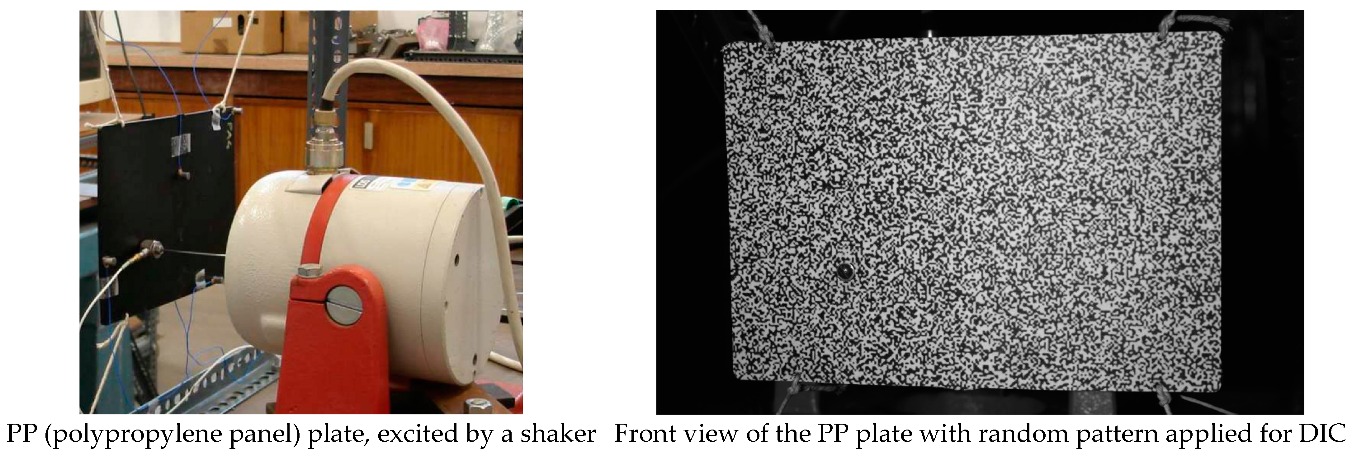
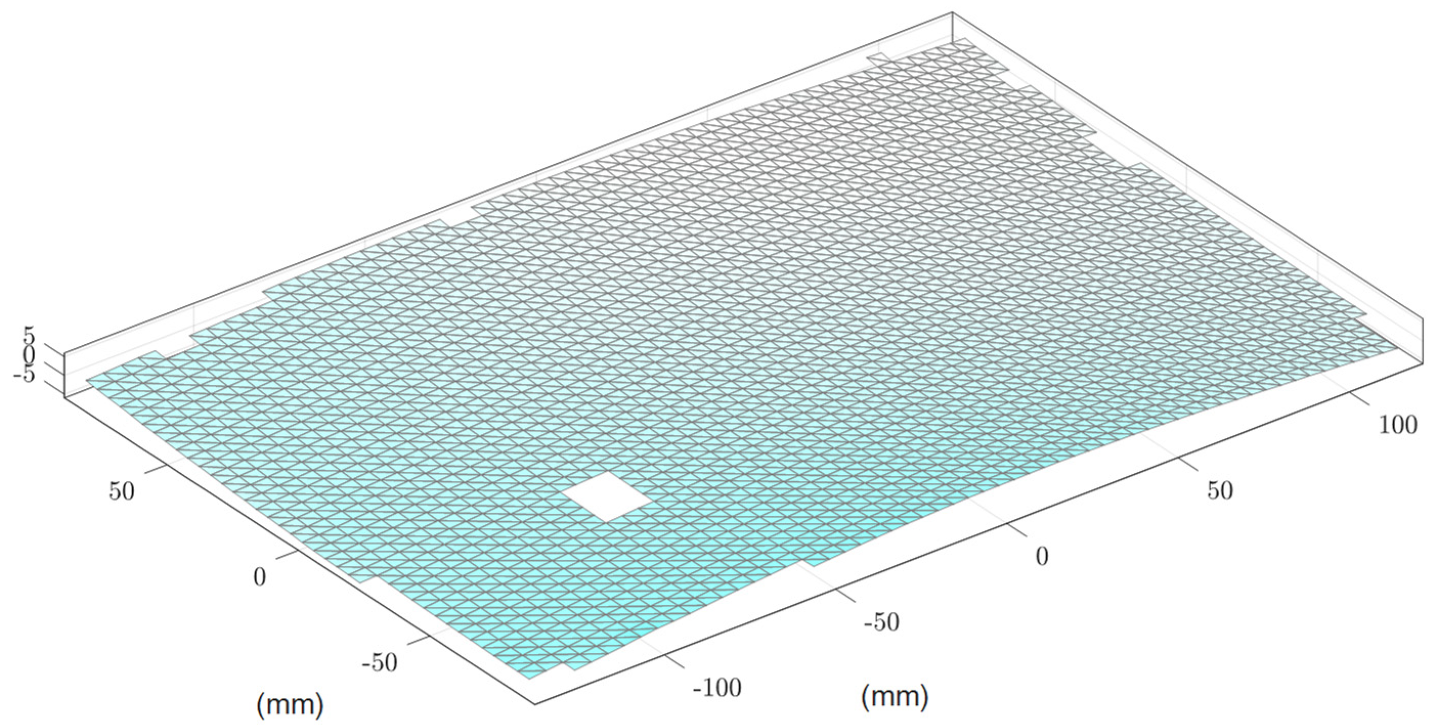
4.1. Experimental Testing Description

The vibration of a polypropylene panel (Sabic Stamax 30YM240) with dimensions of 260 mm × 180 mm × 3 mm, which was slightly curved, was captured using two high-speed CMOS cameras. The panel, which is illustrated in Figure 1, was suspended using four ropes to mimic free boundary conditions. A stinger linked a shaker to the plate, and random excitation in the range of 0–512 Hz was administered. The two high-speed cameras captured transient images at a speed of 1000 frames per second. Images were taken for approximately 4 seconds, resulting in 4004 steps. A DIC algorithm was implemented in the Dantec Dynamics software Istra 4D V4 to estimate the transient displacement from each pair of stereo images. This process generated approximately 2320 data points, also referred to as subset or facet centres, at each temporal step. Furthermore, the force applied by the shaker was recorded during the experiment.

While the plate is nominally flat, it is essential to acknowledge that, post-production, the plate undergoes some degree of distortion, making it not entirely axially symmetric. The utilisation of stereo DIC allows for the capture and measurement of the three-dimensional curved surface of this nominally flat plate, as depicted in Figure 2. Moreover, the benefits of employing stereo DIC extend beyond geometric characterisation, enabling the accurate capture and analysis of out-of-plane deformations and providing a comprehensive understanding of the plate’s behaviour under varying loading conditions.

A 3D surface mesh can be generated by connecting a 3D point cloud through Delaunay triangulation, as illustrated in Figure 2. A small regular void in the bottom left region is observed due to missing DIC information in the measurement. The stereo DIC algorithm effectively captures the curvature of the plate.

The transient displacements at all 2320 DIC subset centres are represented by vectors along the x-, y-, and z-axes. In this study, the primary displacement of interest is the out-of-plane vibration, and thus, the displacement along the normal direction at each point is considered. Therefore, the dataset consists of more than 9 million data points for the 4-second vibration full-field measurement, calculated as the product of 2320 subsets and 4004 steps, expressed as:

$$\mathbf{Z}\equiv \left\{\begin{array}{ccc}\cdots & {\mathbf{z}}_t& \cdots \end{array}\right\}\in {\mathbb{R}}^{2320\times 4004}, t=\left\{\mathrm{1,2},\cdots , 4004 \right\}$$

(15)

This study employs a compressed representation of the shape information using two different methods: data-dependent and data-independent approaches.

4.2. Data-Dependent Basis Function Construction

The data set $\mathbf{Z}$ in Equation (15) can be decomposed into orthonormal basis functions and feature vectors for all temporal snapshots using Singular Value Decomposition, expressed as:

$$\begin{array}{ccccc}\underset{2320\times 4004}{\underbrace{\mathbf{Z}}}& =& \underset{2320\times 2320}{\underbrace{\mathbf{U}}}& \underset{2320\times 4004}{\underbrace{\mathsf{\Sigma }}}& \underset{4004\times 4004}{\underbrace{{\mathbf{V}}^T}}\end{array}$$

(16)

where ${\mathsf{\Phi }}^{PC}\stackrel{\scriptscriptstyle\mathrm{def}}{=}\mathbf{U}$ and ${\mathbf{S}}^{PC}\stackrel{\scriptscriptstyle\mathrm{def}}{=}\mathsf{\Sigma }{\mathbf{V}}^T$ can be considered as the basis functions and feature vectors, respectively. Here, the superscript ‘${ }^{PC}$’ indicates that these basis functions and feature vectors are associated with the principal components.

Figure 3 illustrates the basis functions associated with the 20 largest singular values obtained from SVD. These basis functions are represented by the zero lines, with their values indicated by colour, where yellow represents positive values, and blue represents negative values. The first row’s second column in Figure 3 has no nodal line as it represents the out-of-plane rigid body motion or DC component. It is important to note that the 20 selected terms in this example account for 99.999% of the data set’s nuclear norm, which is defined as the sum of singular values. Therefore, the original data set $\mathbf{Z}$ can be approximated by retaining the sub-space associated with the $r=20$ most significant singular values, expressed as:

$$\begin{array}{ccccccc}\underset{2320\times 4004}{\underbrace{\mathbf{Z}}}& \approx & \stackrel{~}{\underset{2320\times 4004}{\underbrace{\mathbf{Z}}}}& =& \underset{2320\times 20}{\underbrace{{\mathbf{U}}_r}}& \underset{20\times 20}{\underbrace{{\mathsf{\Sigma }}_r}}& \underset{20\times 4004}{\underbrace{{\left[{\mathbf{V}}_r\right]}^T}}\end{array}$$

(17)

i.e., the truncated feature vectors ${\mathbf{S}}_r^{PC}\stackrel{\scriptscriptstyle\mathrm{def}}{=}{\mathsf{\Sigma }}_r{\left({\mathbf{V}}_r\right)}^T$ with a dimensionality of $r=20$ can be used to effectively represent the full-field displacement with a dimensionality of $N=2320$. However, it should be observed that the basis functions associated with lower singular values are influenced by spatial noise, as evident from the last three rows of subplots in Figure 3.

The 20 shape features obtained from principal components, denoted as ${\mathbf{S}}_{20}^{PC}$, will be utilised for the subsequent modal identification in the next section.

4.3. Data-Independent Basis Function Construction

Alternatively, it is possible to construct basis functions on the measured domain (rather than the data itself) using elementary mathematical functions. In this case, a set of two-variable monomials can be defined within the domain of the digital image correlation (DIC) measurements, spanning from zero to ten orders in both variables. To ensure orthonormality, the Gram–Schmidt approach was employed between each monomial. Figure 4 shows 20 of these data-independent basis functions. Notably, these basis functions exhibit a more regular pattern and are less prone to spatial noise compared to the data-dependent basis functions obtained through singular value decomposition (SVD).

Moreover, certain basis functions created using this approach demonstrate usefulness for specific modes. For example, in Figure 4, the first row’s first, second, and third columns of the subplot represent vertical tilting, out-of-plane translation, and horizontal tilting, respectively. If these three features dominate, they could be associated with the rigid body mode of the specimen. These modes might reflect the boundary conditions under which the specimen was constrained, or the vibration induced by external factors such as the cooling fans of the high-speed cameras used for imaging.

The data set $\mathbf{Z}$ can now be projected onto the space spanned by the constructed monomials. The resulting projections are referred to as the adaptive geometric moment descriptor (AGMD). This can be expressed as ${\mathbf{z}}_t={\mathsf{\Phi }}^{AGMD}{\mathbf{s}}_t^{AGMD}$ for individual temporal snapshots, or for the entire data set as:

$$\begin{array}{cccc}\underbrace{\mathbf{Z}}& \cong & \underbrace{{\mathsf{\Phi }}_{}^{AGMD}}& \underbrace{{\mathbf{S}}_{}^{AGMD}}\\ 2320\times 4004& & 2320\times R& R\times 4004\end{array}$$

(18)

where $R$ represents the total number of constructed monomials which, in this case, is determined by the combination of $m=0:8$ and $n=0:10$, resulting in $R=9\times 11=99$. Of course, if more higher-order monomials were included, both sides of Equation (18) would be closer.

However, as mentioned earlier in Equation (16), it is desirable to retain a reduced number of features ($r\ll R$) while still preserving the full-field displacement shape. The reduced dimensionality $r$ can be determined by selecting the best combination of $r$ columns from ${\mathsf{\Phi }}^{AGMD}$, denoted as ${\mathsf{\Phi }}_r^{AGMD}$, such that the Frobenius norm of the error ${‖\mathbf{Z}-{\mathsf{\Phi }}_r^{AGMD}{\mathbf{S}}_r^{AGMD}‖}_F$ is the minimum. Here, ${\mathbf{S}}_r^{AGMD}$ represents the corresponding $r$ rows of the feature matrix ${\mathbf{S}}_{}^{AGMD}$. Another metric that can be used to determine the retaining dimensionality is by selecting the $r$ maximum $L_2$ norm of the row vectors in the shape feature matrix ${\mathbf{S}}^{AGMD}$, ensuring that the correlation between the original shape and the reconstruction, denoted as $\mathrm{c}\mathrm{o}\mathrm{r}\mathrm{r}\left(\mathbf{Z},{\mathsf{\Phi }}_r^{AGMD}{\mathbf{S}}_r^{AGMD}\right)$, exceeds a specified threshold, such as 99%. The orthonormality of the constructed basis functions ${\mathsf{\Phi }}^{AGMD}$ allows us to consider the “energy” of the shapes as the L2 norms of the shape feature vectors.

As this set of basis functions is data-independent, a slightly higher number of terms will be retained than in the previous data-dependent case. In this study, $r=25$ was selected and denoted as ${\mathbf{S}}_{25}^{AGMD}$.

Figure 5 illustrates a comparison between the full-field displacement obtained from digital image correlation measurements and the reconstructed displacement field using only 25 terms of the data-independent shape descriptors AGMD. The DIC measurement provides displacement data at 2320 spatial points for each time step. The correlation between the reconstructed displacement field and the DIC measurements is evaluated for each temporal step. The obtained correlation values exceed 99.65% for all steps, indicating a strong agreement between the two datasets. Moreover, most correlation values are greater than 99.99%, indicating an excellent match between the reconstructed displacement field and the DIC measurements.

The shape compression ratio, defined as the ratio of the number of shape descriptors (25) to the number of measurements (2320), is approximately 1%. It indicates that the AGMD approach substantially reduces data size while maintaining high accuracy in representing the displacement field. The next section will use these 25 shape features obtained from the AGMD approach for the subsequent modal identification.

5. Modal Identification in Feature Space and Results

This section discusses vibration modal identification using low-dimensional shape-preserving feature spaces. The state space formulation is used for identification, with force history considered as the input. The shape features are treated as the outputs. The identification algorithm is fed with data-dependent and data-independent features. A comparison is made between the identified modal properties obtained from the two sets of shape features.

5.1. Shape Feature State Space

Now, the task of modal identification can be carried out in the dimensionally reduced feature space. For example, if we consider the state space formulation as given in Equations (2)–(4), the state vector $\mathbf{x}$ and output vector $\mathbf{y}$ can be mapped to the shape feature sub-space ${\mathsf{\Phi }}_r$, which can be either ${\mathsf{\Phi }}_r^{PC}$ or ${\mathsf{\Phi }}_r^{AGMD}$, as discussed in the previous section. The shape feature space is constructed based on the spatial domain and is independent of temporal operations. Taking the time derivative of both sides Equation (5), we have $\dot{\mathbf{z}}=\mathsf{\Phi }\dot{\mathbf{s}}$.

Next, we can construct a diagonal block matrix $\mathsf{\Psi }$ to map the state vectors in the data domain to the feature space, expressed as:

$$\mathbf{x}=\mathsf{\Psi }\mathcal{s}$$

(19)

or in block-wise expression:

$$\left\{\begin{array}{c}\mathit{z}\\ \dot{\mathit{z}}\end{array}\right\}=\left[\begin{array}{cc}{\mathsf{\Phi }}_r& 0\\ 0& {\mathsf{\Phi }}_r\end{array}\right]\left\{\begin{array}{c}{\mathbf{s}}_r\\ {\dot{\mathbf{s}}}_r\end{array}\right\}$$

(20)

By substituting Equation (19) into Equation (2) and pre-multiplying by the transpose of the mapping matrix $\mathsf{\Psi }$, we obtain the following expression due to the orthonormality of the constructed basis in ${\mathsf{\Phi }}_r$:

$$\dot{\mathcal{s}}=\overline{\mathbf{A}}\mathcal{s}+\overline{\mathbf{B}}\mathbf{u}$$

(21)

where $\overline{\mathbf{A}}={\mathsf{\Psi }}_r^T\mathbf{A}{\mathsf{\Psi }}_r$ and $\overline{\mathbf{B}}={\mathsf{\Psi }}_r^T\mathbf{B}$. The output equation (Equation (4)) in the data space may also be formulated in the shape feature space as:

$${\mathbf{y}}_{\mathbf{s}}={\mathbf{C}}_{\mathbf{s}}\mathcal{s}$$

(22)

where ${\mathbf{y}}_{\mathbf{s}}$ is the ‘measured’ output and ${\mathbf{C}}_{\mathbf{s}}$ is the measurement matrix in the feature space. In this study, the shape feature vectors ${\mathbf{s}}^{PC}$ or ${\mathbf{s}}^{AGMD}$ will be used as the feature output for the modal identification, i.e., ${\mathbf{C}}_{\mathbf{s}}=\left[\begin{array}{ccc}0& ⋮& \mathbb{I}\end{array}\right].$ Therefore, the transfer function in the shape feature space may be expressed as:

$$\overline{\mathbf{G}}\left(\mathfrak{s}\right)={\mathbf{C}}_{\mathbf{s}}{\left(\mathfrak{s}\mathbb{I}-\overline{\mathbf{A}}\right)}^{-1}\overline{\mathbf{B}}$$

(23)

Subsequently, the modal properties may be extracted from Equation (23) via some commonly used method, e.g., least squares curve fitting [59]. It should be noted that the identified mode shapes ${\mathsf{\phi }}_s$ from Equation (23) lie in the feature space. The full field mode shapes $\mathsf{\phi }$ in the data space, i.e., the cartesian space, can be reconstructed via the basis functions as:

$$\mathsf{\phi }={\mathsf{\Phi }}_{\mathit{r}}{\mathsf{\phi }}_{\mathbf{s}}$$

(24)

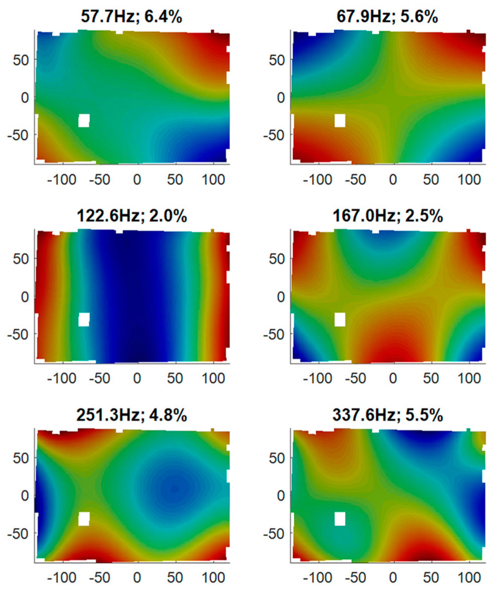
5.2. Identification Results of the Study Case

In this subsection, the modal identification results using principal component (PC) features and adaptive geometric moment descriptor (AGMD) features are presented. As discussed above, the identification process was carried out based on the dimensionally reduced feature spaces. A comparison between the two sets of results will also be discussed.

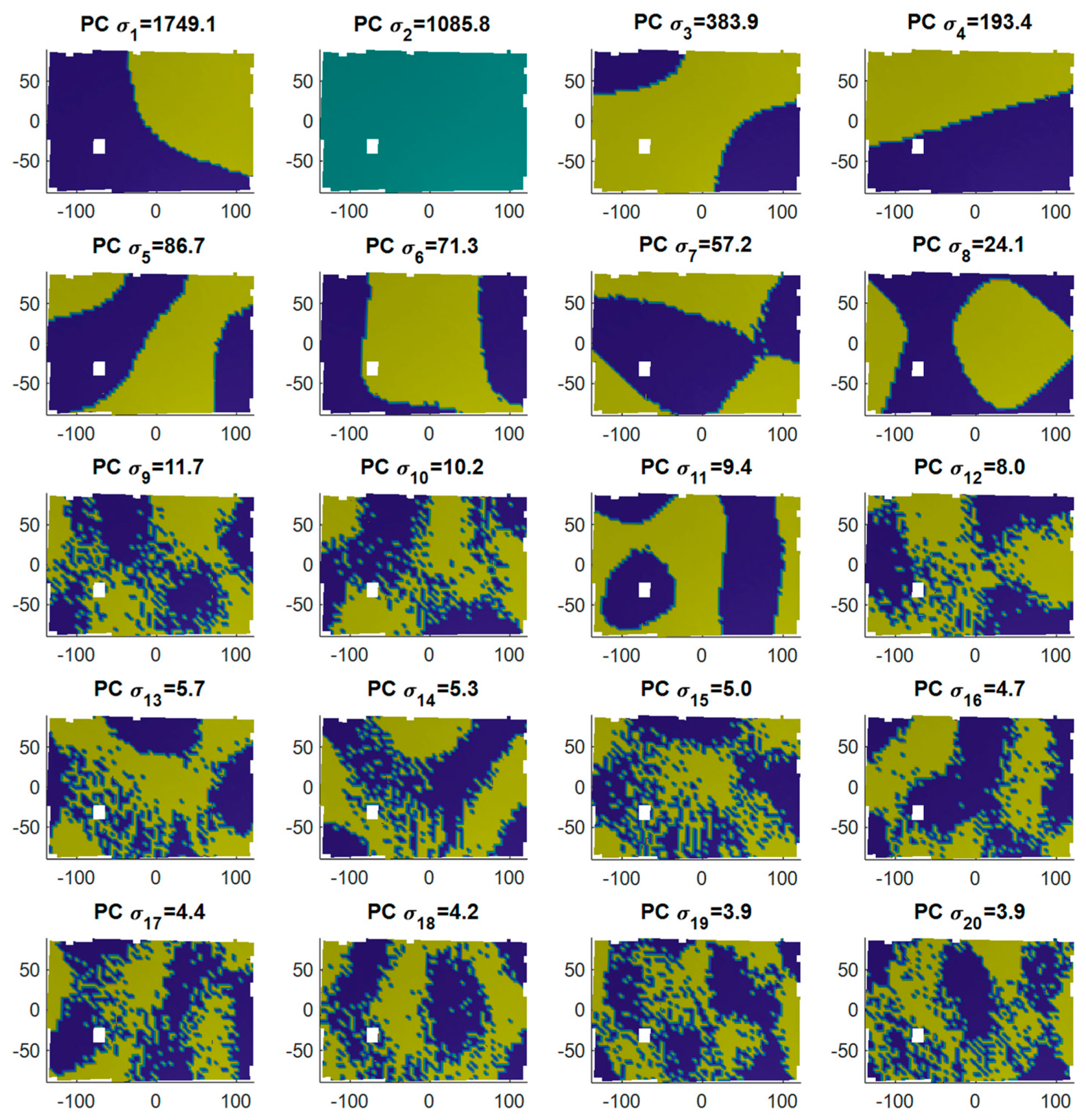
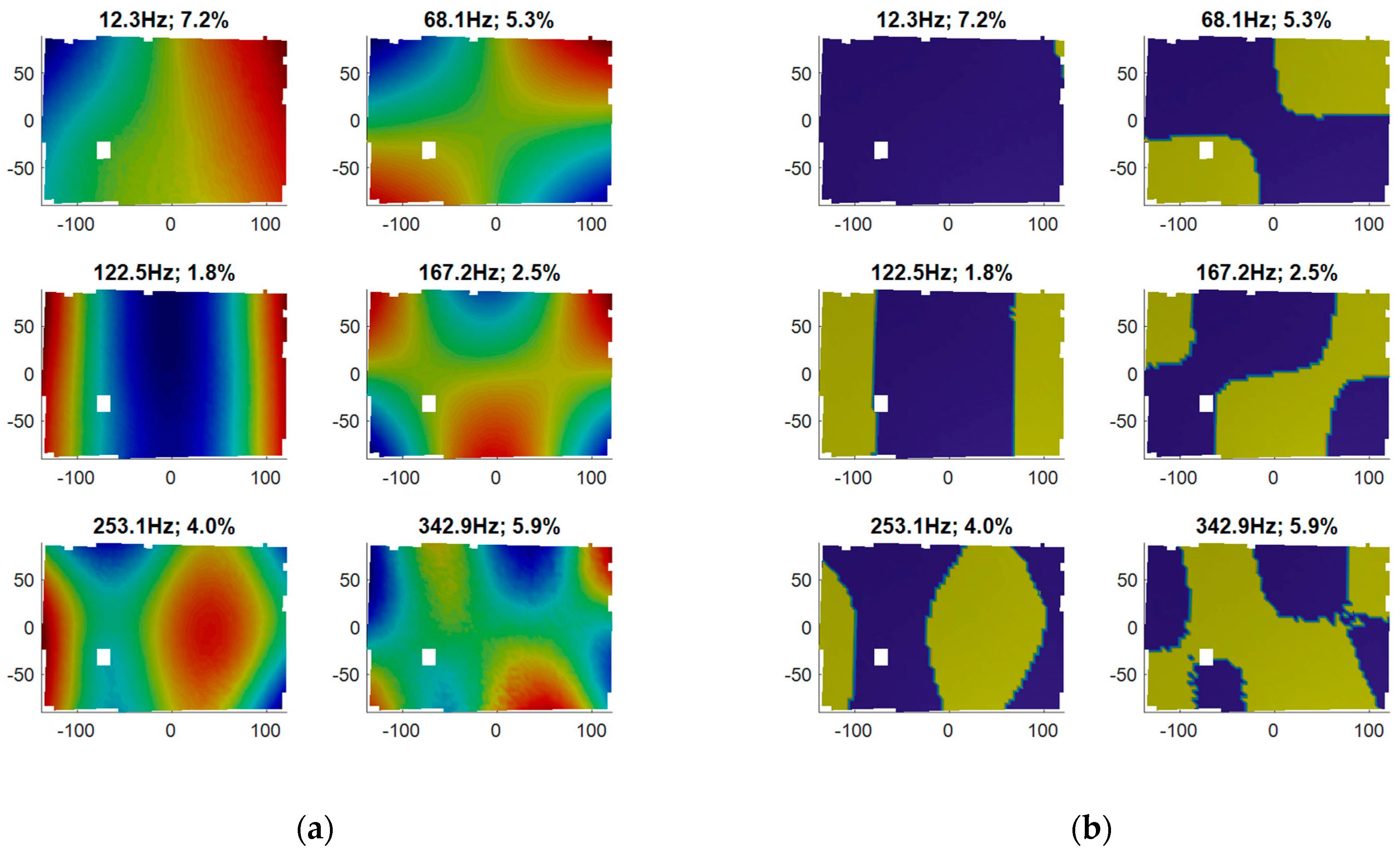
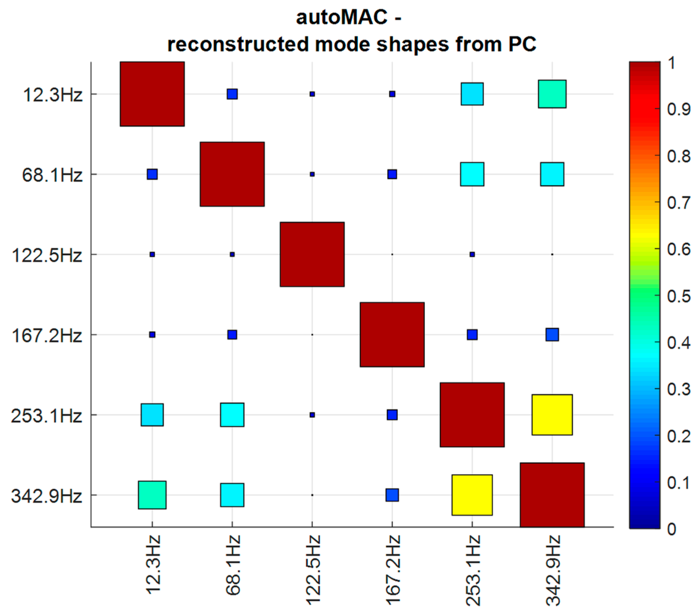
5.2.1. By PC features

By Equation (17), it is observed that using only 20 PC features captures over 99.999% of the nucleus norm of the data matrix. The resulting modal properties effectively represent the full-field mode shapes, as demonstrated in Figure 6. Notably, six modes have been identified within the frequency range of 0–350 Hz, with consideration that the random excitation spanned 0–512 Hz. Figure 6a shows the reconstructed full-field mode shapes comprising 2320 data points for each pattern using the 20-term feature mode shape described in Equation (24). The identified natural frequencies and damping ratios are indicated in the titles above each mode shape pattern. Conversely, Figure 6b shows the same mode shapes, emphasising only the nodal lines and deflection signs (yellow in one direction, blue in the opposite).

To simulate a “free–free” boundary condition, the plate was constrained by four ropes at its corners. Based on the plots in Figure 6, the first and second horizontal bending modes can be observed at 122.5 Hz and 253.1 Hz, respectively. Additionally, the first, second, and third twisting modes are observed at 68.1 Hz, 167.2 Hz, and 342 Hz, respectively. However, the mode at 12.3 Hz does not exhibit clear deformation or nodal lines. It is plausible that this mode corresponds to a pseudo-rigid-body mode associated with the constraints/boundary conditions imposed by the four ropes.

The higher-mode patterns and nodal lines exhibit some spatial noise, which may be influenced by the noisy basis functions constructed from the principal components, as depicted in Figure 3.

Figure 7 shows an autoMAC plot for the PC-reconstructed modes, representing the modal assurance criteria comparison between the full-field mode shapes reconstructed from the identified feature modes. The plot exhibits a distinct diagonal grid with nearly MAC 1 values and small or zero off-diagonal terms, indicating the high quality of the identified mode shapes.

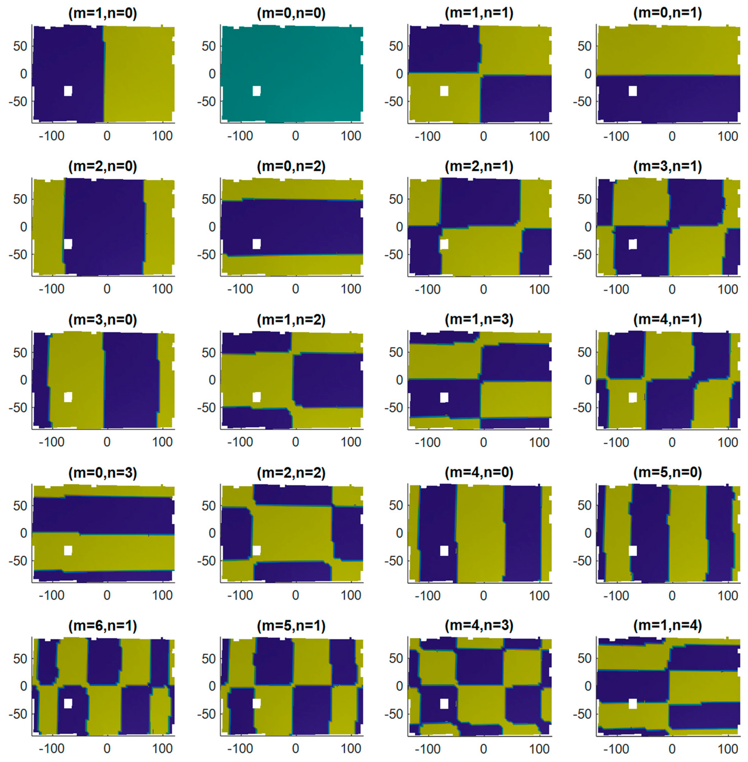
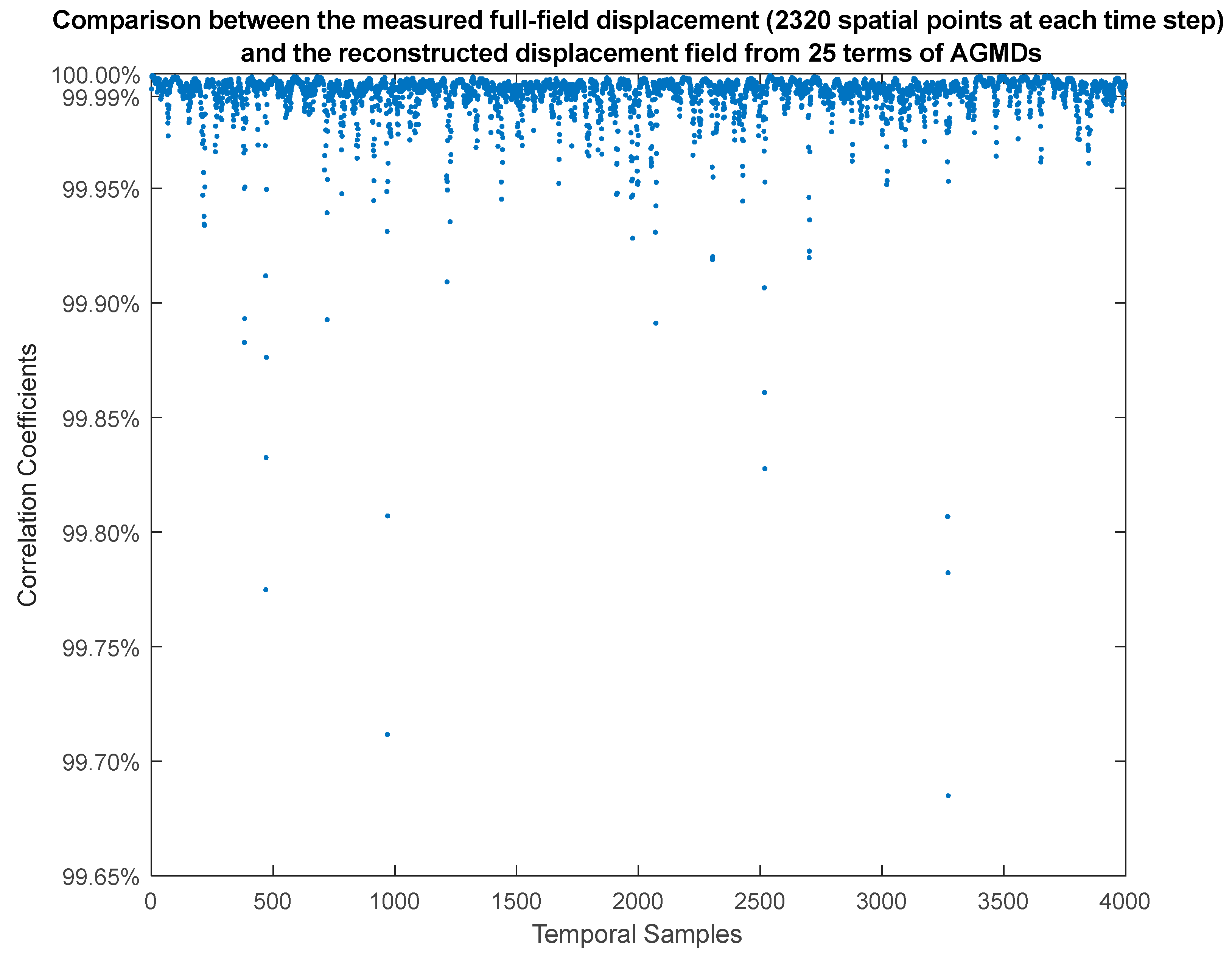
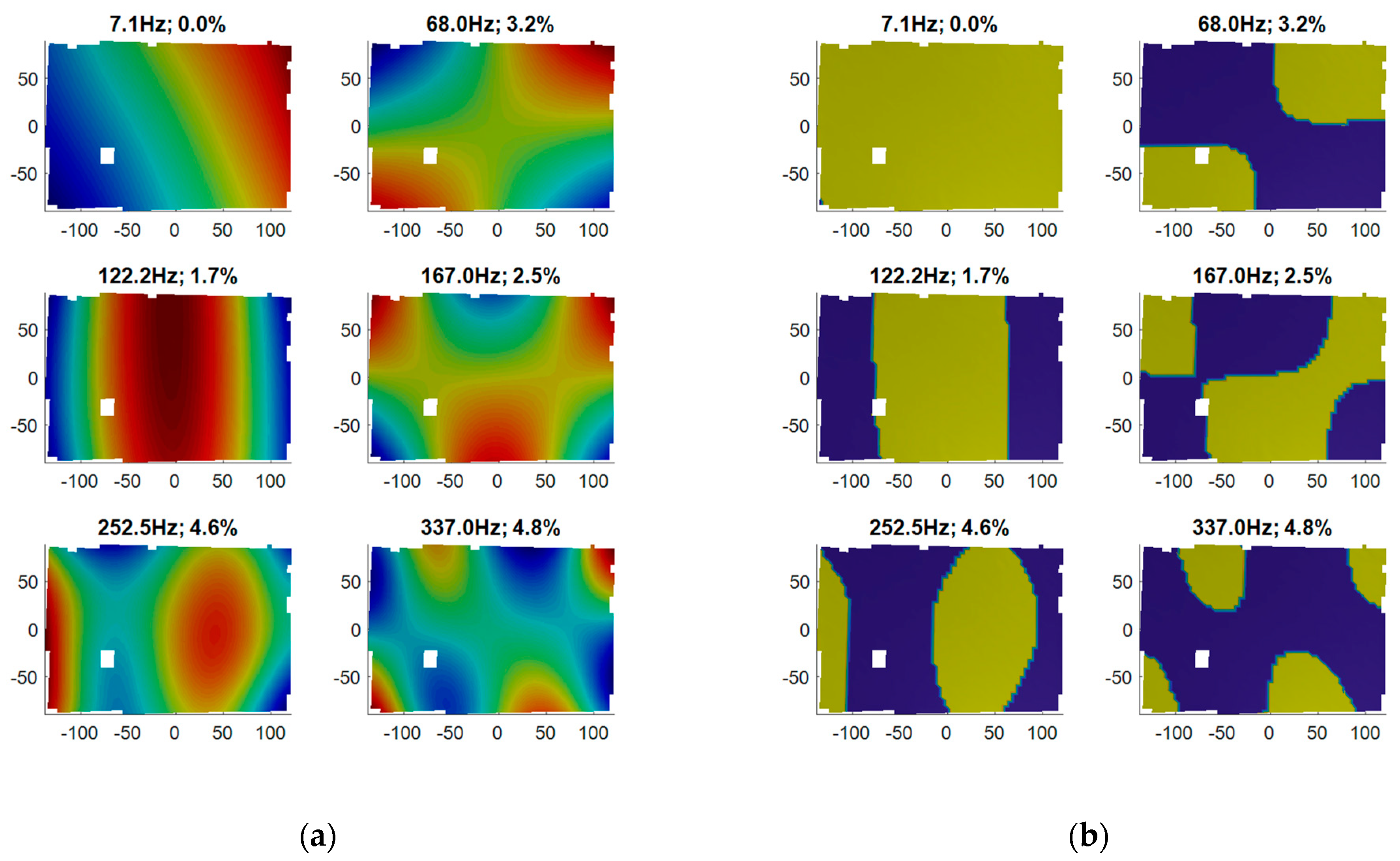
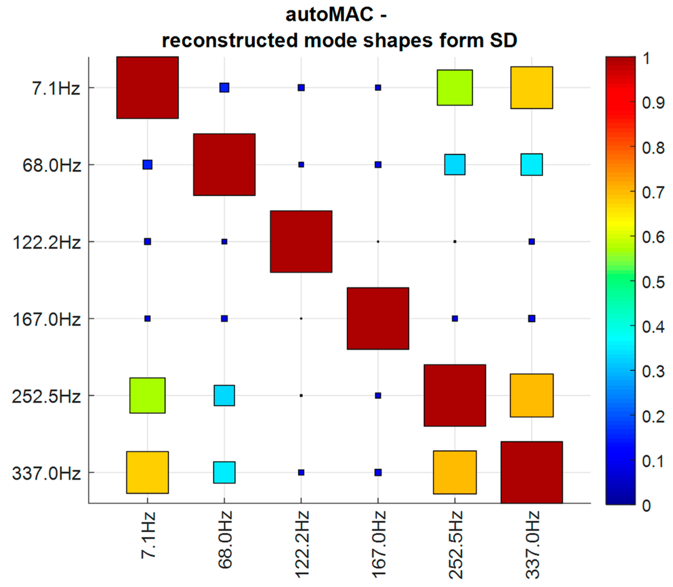
5.2.2. By AGMD Features

Figure 8 illustrates the modal properties identified from 25 terms of AGMD features. Subplot (a) displays the full-field mode shape patterns, while subplot (b) highlights the corresponding nodal lines. The titles provide the natural frequencies and modal damping ratios. Similar to Figure 6, the identified modes include a pseudo-rigid-body mode, two bending modes, and three twisting modes.

Figure 9 shows the autoMAC plot, comparing the full-field mode shapes reconstructed from the low-dimensional feature mode shapes. The plot demonstrates a clear diagonal unity grid, indicating a high level of agreement among the identified mode shapes. It confirms the reliability and accuracy of the mode identification results obtained from AGMD features.

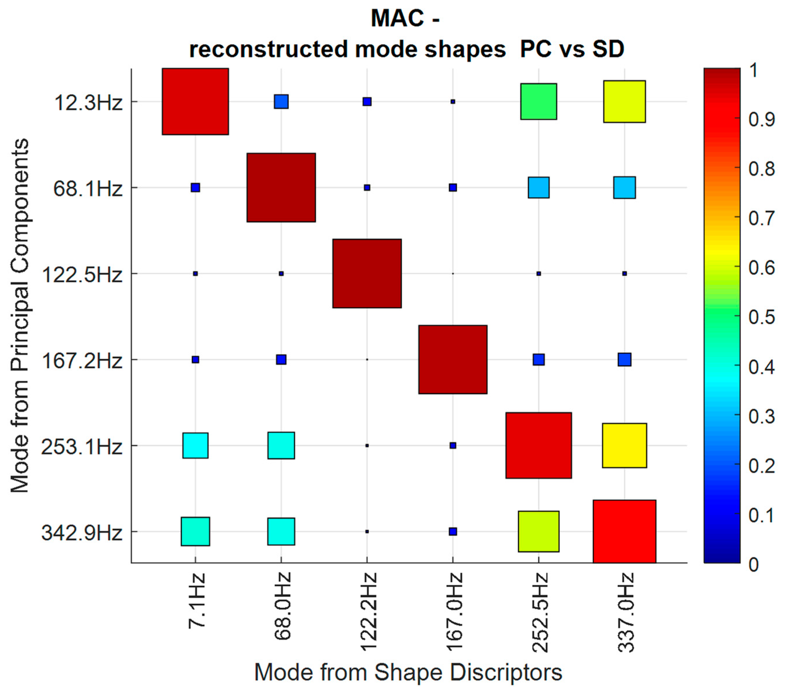
5.2.3. Comparison between the Two

Figure 10 shows a MAC comparison of the reconstructed mode shapes (2320-dimensional) between the identified modes. The vertical axis represents the reconstructed mode shapes from the 20-dimensional PC modes, while the horizontal axis represents the reconstructed mode shapes from the 25-dimensional AGMD modes. The identified natural frequencies are compared and presented in

Table 1. Identified natural frequencies comparisons (the percentage difference was calculated from difference over average).

#	20PCs	25AGMDs	Diff.	Diff.
	Hz	Hz	Hz	%
1	12.3	7.1	5.2	53.61%
2	68.1	68.0	0.1	0.15%
3	122.5	122.2	0.3	0.25%
4	167.2	167.0	0.2	0.12%
5	253.1	252.5	0.6	0.24%
6	342.9	337.0	5.9	1.74%

. It is worth noting that the AGMD basis functions, being data-independent, required a slightly higher number of terms compared to the PC basis functions, which are data-dependent. Most of the identified modes exhibit a high level of agreement between the two feature compression methods. However, there are some differences observed in modes 1 and 6.

For mode 6, a visual comparison of the mode shape patterns in the bottom-right corners of Figure 6 and Figure 8 suggests that the AGMD-based mode shape is slightly better due to its pattern symmetry and less noisy nodal lines. This difference can be attributed to the influence of data noise on the basis functions constructed by PC or SVD, whereas AGMD basis functions are more robust to spatial noise since they are independently constructed from the data.

Regarding mode 1, which represents the pseudo-rigid-body mode located at the top-left corners of Figure 6 and Figure 8, it can be observed that the AGMD-based identification exhibits more straight “contour lines”, indicating a more rigid motion compared to the PC-based identification. This characteristic is also reflected in the corresponding basis functions. For example, in the first row of Figure 3 and Figure 4, the AGMD basis functions exhibit more rigid behaviour, such as vertical tilting, out-of-plane translation, and horizontal tilting, which align with the nature of the pseudo-rigid-body mode resulting from the boundary conditions.

The agreement between the two sets of identified modes is remarkably consistent for modes 2 to 6, showcasing the effectiveness of our methodology. However, the first mode, as depicted in of Figure 6 and Figure 8 through nodal line plots, stands out due to its distinct characteristics. This mode can be interpreted as the rigid-body mode for the plate, primarily arising from the constraints imposed by the four strings that connect the plate to a rigid aluminium frame on the workbench. It is essential to clarify that the data provided to the MATLAB identification function comprised the shape features of the plate. Our chosen identification algorithm employed a global approach with increasing order iterations. Consequently, while the identified modes exhibit strong agreement with the genuine plate deformation modes, they might not accurately capture the pseudo-rigid mode represented by the first mode. Therefore, the first mode’s accuracy may not align as closely with the other five plate deformation modes. Furthermore, this discrepancy is reflected in the relatively high modal assurance criterion (MAC) values when comparing the first mode to the sixth mode. This phenomenon can be attributed to the comparison domain’s focus on the plate itself, excluding the constraining strings. Thus, the elevated MAC values between mode 1 and mode 6 likely arise from localized similarities in a subdomain, despite the fundamental differences between these two modes.

6. Mode Shape Expansion from QR-Pivot Sensors Placement

6.1. A Brief Review of Sensor Placement

In applications like structural health monitoring, continuous online measurement is often necessary [73,74]. Utilising point-wise sensors on structures proves to be more practical than employing high-speed cameras throughout the operational period. It becomes crucial to optimally place a limited number of these sensors to capture as much information as possible. Subsequently, the reconstructed shape features obtained from these limited point sensors can expand the full field displacement [75,76]. The strain field may also be estimated from the reconstructed displacement fields [77,78].

In optimal sensor placement problems, the concept of effective independence (EfI), introduced by Kammer [79,80,81], addresses the problem by optimising a norm of the Fisher information matrix (FIM), e.g., its determinant. The FIM may be expressed as the inner product of mode shape vectors divided by the covariance of the measurement noise. However, the EfI approach may suffer from a poor signal-to-noise ratio (SNR) when the locations determined by independence exhibit low-energy responses. Alternative methods, such as the driving point residue (DPR) and kinetic energy-based methods [82], have been proposed to overcome this issue. Both methods require mode shape patterns obtained from numerical methods, such as finite element (FE) models. Another approach that involves the independence measurement of FE mode shape vectors is the modal assurance criteria (MAC) [82,83]. The sensor placement problem can be formulated by minimising the off-diagonal terms in the MAC matrix [84].

Another important alternative approach involves formulating the sensor placement based on the concept of information entropy [85,86,87], which characterises the uncertainty in the modal parameters. The goal is to search for a sensor configuration that minimises the change in information entropy [88]. This approach can be solely based on a nominal model, such as an FE model.

6.2. Data-Driven Approach for Sensor Placement Using QR-Pivots

In this section, the sensor placement problem is handled from a data-driven perspective rather than a nominal model-driven approach. This approach differs as a set of compact basis functions has already been created to expand full-field displacements and mode shapes accurately. The objective is to suggest the placement of p-pointwise sensors, allowing their measured responses to estimate the feature vector within the space expanded by the basis functions. Subsequently, the full-field displacement can be expanded using the estimated feature vector multiplied by the basis functions.

In the following example, an approach based on the QR decomposition algorithm via the pivoting method will be applied to determine the optimal locations for the point-wise sensors. Consider the feature space approximation ${\mathbf{z}}_t\cong {\mathsf{\Phi }}_r{\mathbf{s}}_t$ within the framework of compressed sensing (CS) [63,64,89], assuming that the feature vector ${\mathbf{s}}_t$ is sparse. In this case, only a smaller number of responses ${\mathbf{w}}_t$ need to be measured, while the high-dimensional data ${\mathbf{z}}_t$ can still be reconstructed. The mathematical relations can be expressed as follows:

$${\mathbf{w}}_t={\mathbf{L}}_0{\mathbf{z}}_t\cong {\mathbf{L}}_0{\mathsf{\Phi }}_r{\mathrm{s}}_{\mathrm{t}}\equiv \mathsf{\Theta }{\mathbf{s}}_t$$

(25)

where ${\mathbf{L}}_0$ may be called the “measurement” matrix. In compressed sensing, the basis function matrix ${\mathsf{\Phi }}_r$ (also known as dictionaries) is typically universal and redundant. To ensure accurate reconstruction, an incoherent measurement matrix ${\mathbf{L}}_0$ needs to be designed to satisfy the restricted isometry property (RIP) [69,90,91]. For example, a random matrix ${\mathbf{L}}_0$ can be used in comparison to Fourier or wavelet basis matrices ${\mathsf{\Phi }}_r$. The K-sparse feature vector ${\mathbf{s}}_t$ can then be recovered using optimisation algorithms such as LASSO [90]. Finally, the signal ${\mathbf{z}}_t$ can be reconstructed by multiplying the basis functions with the recovered feature vector.

However, in this study, the basis functions are tailored to the problem, and the dimension of the feature vector is already small instead of being sparse. In this case, we refer to the matrix ${\mathbf{L}}_0$ as the point-wise sensor placement/locating matrix, with dimensions of $p\times N$, where $p$ is the number of sensors to be placed. The placement matrix ${\mathbf{L}}_0$ consists of elementary row vectors with zero elements except for a single unity at the column corresponding to the degree of freedom for the sensor. The number of sensors $p$ and the dimension of the retained shape feature $r$ can be similar, i.e., $p \ge r$, but both $p$ and $r$ are much smaller than $N$.

Once the measurement ${\mathbf{w}}_t$ ($p\times 1$ vector at each time step) is captured, the corresponding shape feature vector ${\mathbf{s}}_t$ can be obtained by pseudo-inverting the matrix $\mathsf{\Theta }$ in Equation (25), i.e.,:

$${\widehat{\mathbf{s}}}_t={\mathsf{\Theta }}^{†}{\mathbf{w}}_t={\left({\mathbf{L}}_0{\mathsf{\Phi }}_r\right)}^{†}{\mathbf{w}}_t$$

(26)

Subsequently, the full-field displacement ${\mathbf{z}}_t$ (an $N\times 1$ vector) can be reconstructed as ${\widehat{\mathbf{z}}}_t={\mathsf{\Phi }}_r{\widehat{\mathbf{s}}}_t$.

To determine an optimal placement matrix ${\mathbf{L}}_0$ with dimensions $p\times N$, the goal is to select the best combination of $p$ rows from the tailored basis function matrix ${\mathsf{\Phi }}_r\in {\mathbb{R}}^{N\times r}$. This selection is crucial as the matrix $\mathsf{\Theta }$, represented as $\mathsf{\Theta }\equiv {\mathbf{L}}_0{\mathsf{\Phi }}_r$ in Equation (25), needs to be inverted. Therefore, the sensor selection problem is about identifying the $p$ rows of ${\mathsf{\Phi }}_r$ that effectively optimise the condition of the matrix $\mathsf{\Theta }$ for its inversion. The selection can be represented using the Boolean matrix ${\mathbf{L}}_0$, expressed using canonical basis vectors ${\mathbf{e}}_j\in {\mathbb{R}}^N$ as shown below:

$${\mathbf{L}}_0={\left[\begin{array}{cccc}{\mathbf{e}}_{\gamma 1}& {\mathbf{e}}_{\gamma 2}& \cdots & {\mathbf{e}}_{\gamma p}\end{array}\right]}^T$$

(27)

One approach for constructing ${\mathbf{L}}_0$ is to select the most independent rows from ${\mathsf{\Phi }}_r$. When $p=r$, it may be expressed as:

$${\gamma }_{*}=\underset{\gamma ,\left|\gamma \right|=p}{\mathrm{argmax}} \left(\det \mathsf{\Theta }\left(\gamma \right)\right)=\underset{\gamma ,\left|\gamma \right|=p}{\mathrm{argmax}} \left( \prod _i{\sigma }_i\left(\mathsf{\Theta }\left(\gamma \right)\right)\right)$$

(28)

or, if $p>r$:

$${\gamma }_{*}=\underset{\gamma ,\left|\gamma \right|=p}{\mathrm{argmax}} \left(\det \left({\mathsf{\Theta }}^T\mathsf{\Theta }\right)\right)=\underset{\gamma ,\left|\gamma \right|=p}{\mathrm{argmax}} \left( \prod _i{\sigma }_i\left({\mathsf{\Theta }}^T\mathsf{\Theta }\right)\right)$$

(29)

where $\mathrm{d}\mathrm{e}\mathrm{t}\left(\right)$ denotes the determinant of a matrix, and ${\sigma }_i\left(\right)$ denotes the $i^{th}$ singular value of the matrix. The studies by Monohar et al. [92] and Drmac and Gugercin [93] show that the QR decomposition, with column pivoting, approximates the greedy solution of Equation (28) or (29).

The column pivot method in QR decomposition starts with the first column and sequentially selects the next pivot column based on its correlation with the previous columns. Columns that correlate less with the previously processed columns are preferred as pivots. This selection strategy helps to maximise the independence among the selected columns, leading to improved numerical stability in the decomposition.

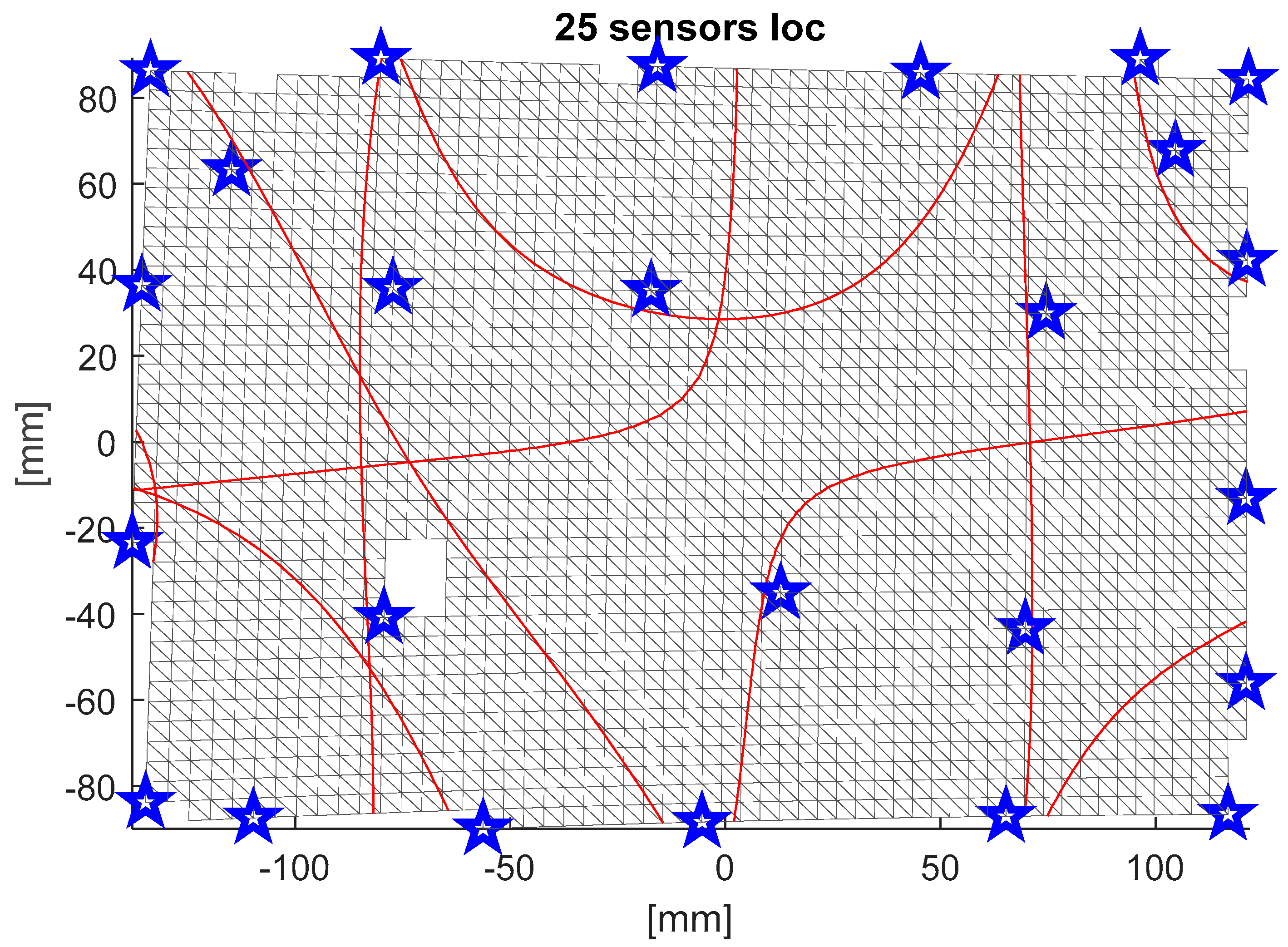
6.3. Application Example on the Plate’s Sensor Placement

In this case study, it is assumed that the number of point-wise sensors, $p$, is equal to the dimension of the retained shape features $r$, i.e., $p=r=25$. The basis functions used in this study are AGMD basis functions. The sensor locations obtained from QR decomposition pivots may be implemented via the MATLAB function [Q, R,${\mathbf{p}}_0$] = qr(${\mathsf{\Phi }}_r^T,$ ‘vector’). The function returns a permutation vector ${\mathbf{p}}_0$ for the pivots. Therefore, the ‘nearly optimal’ row selection from the basis function can be expressed using MATLAB’s matrix syntax, as:

$${\mathsf{\Theta }}_{\mathbf{*}}={\mathbf{L}}_0{\mathsf{\Phi }}_r={\mathsf{\Phi }}_r\left({\mathbf{p}}_0,:\right)$$

(30)

The locations of the $p=25$ sensor locations from the pivot vector ${\mathbf{p}}_0$ are depicted as blue pentagrams in Figure 11.

For verification purposes, the displacement time history, denoted as $\mathbf{W}=\mathbf{Z}\left({\mathbf{p}}_0,:\right)\in {\mathbb{R}}^{25\times 4004}$, was extracted at the locations corresponding to the pentagrams. These 25 points were then utilised for modal identification, similar to the previous sections’ approach for shape features. The estimated modal frequencies and shapes for the 25 degrees of freedom associated with the point-wise sensors are represented as $f_n^w$ and ${\mathit{\phi }}_n^w$, respectively.

To expand the full-field mode shape ${\mathit{\phi }}_n^Z$, the following relationship is applied:

$${\mathit{\phi }}_n^Z={\mathsf{\Phi }}_r{\widehat{\mathbf{s}}}_n^w$$

(31)

where the feature mode shape ${\widehat{\mathbf{s}}}_n^w$ is estimated by:

$${\widehat{\mathbf{s}}}_n^w={\mathsf{\Theta }}_{\mathrm{*}}^{-1}{\mathit{\phi }}_n^w$$

(32)

Figure 12 illustrates the expanded full-field mode shapes ${\mathit{\phi }}_n^Z$, which consist of 2320 degrees of freedom. These expanded mode-shape patterns are derived from the mode shape ${\mathit{\phi }}_n^w$ obtained from the 25 point-wise sensors. Notably, the expanded mode shapes exhibit a remarkable similarity to the full-field mode shapes presented in Figure 8, where the full-field identification process was conducted. This similarity indicates a strong agreement and correspondence between the expanded mode shapes and the original full-field mode shapes. Then, applications such as full-field strain map analysis could be carried out from only 25 sparse point-wise sensors.

To further quantify the agreement between the two sets of mode shapes, a MAC plot is presented in Figure 13. In this plot, the vertical modes correspond to the 25 point-wise sensors, while the horizontal modes represent the 25 terms of AGMDs. The majority of the modal properties demonstrate a high level of agreement between the two sets. However, it is observed that the first mode does not align well, implying that the pseudo-rigid-body mode identified by the AGMD was not accurately captured by the 25 point-wise ‘sensors’.

7. Conclusions

This paper has explored two approaches for creating a feature space to compress full-field vibration measurements. Despite its sensitivity to measurement noise and potential insensitivity to weakly excited modes, the data-dependent approach offers an effective means of dimensionality reduction. Conversely, the data-independent approach provides greater flexibility in constructing patterns based on user preferences and judgments. In the case study, the creation of dedicated rigid-body mode patterns demonstrated the capability of the approach to accurately reflect resonant modes from the specimen’s support while also exhibiting improved robustness to measurement noise.

Both approaches facilitate efficient modal identification by utilising compressed spatial features instead of raw and high-dimensional spatial snapshots, thereby overcoming potential computational challenges. Moreover, the constructed feature space enables a data-driven approach to optimising point-wise sensor placement, eliminating the reliance on conventional strategies based on nominal models. The case study validated the effectiveness of this two-stage approach for identification and monitoring applications, involving an offline full-field approach and online long-term monitoring using point-wise sensors.

References

1. Ewins, D.J. Modal Testing: Theory, Practice, and Application, 2nd ed.; John Wiley & Sons: Hoboken, NJ, USA, 2000. [Google Scholar]
2. Mottershead, J.E.; Link, M.; Friswell, M.I. The sensitivity method in finite element model updating: A tutorial. Mech. Syst. Signal Process. 2010, 25, 2275–2296. [Google Scholar] [CrossRef]
3. Mares, C.; Friswell, M.; Mottershead, J. Model updating using robust estimation. Mech. Syst. Signal Process. 2002, 16, 169–183. [Google Scholar] [CrossRef]
4. Behmanesh, I.; Moaveni, B.; Lombaert, G.; Papadimitriou, C. Hierarchical Bayesian model updating for structural identification. Mech. Syst. Signal Process. 2015, 64–65, 360–376. [Google Scholar] [CrossRef]
5. Deraemaeker, A.; Reynders, E.; De Roeck, G.; Kullaa, J. Vibration-based structural health monitoring using output-only measurements under changing environment. Mech. Syst. Signal Process. 2008, 22, 34–56. [Google Scholar] [CrossRef]
6. Sohn, H.; Farrar, C.R. Damage diagnosis using time series analysis of vibration signals. Smart Mater. Struct. 2001, 10, 446–451. [Google Scholar] [CrossRef]
7. Kamariotis, A.; Chatzi, E.; Straub, D. A framework for quantifying the value of vibration-based structural health monitoring. Mech. Syst. Signal Process. 2023, 184, 109708. [Google Scholar] [CrossRef]
8. Farrar, C.R.; Worden, K. An introduction to structural health monitoring. Philos Trans A Math Phys Eng Sci. 2007, 365, 303–315. [Google Scholar] [CrossRef] [PubMed]
9. Farrar, C.R.; Worden, K. Structural Health Monitoring: A Machine Learning Perspective; John Wiley & Sons: Hoboken, NJ, USA, 2012. [Google Scholar]
10. Ren, W.-X.; De Roeck, G. Structural Damage Identification using Modal Data. I: Simulation Verification. J. Struct. Eng. 2002, 128, 87–95. [Google Scholar] [CrossRef]
11. Ram, Y.M.; Mottershead, J.E. Receptance Method in Active Vibration Control. AIAA J. 2007, 45, 562–567. [Google Scholar] [CrossRef]
12. Preumont, A. Vibration Control of Active Structures: An Introduction; Springer: Berlin/Heidelberg, Germany, 2018. [Google Scholar]
13. Mottershead, J.E.; Tehrani, M.G.; Ram, Y.M. An Introduction to the Receptance Method in Active Vibration Control. In Proceedings of the IMAC-XXVII, Orlando, FL, USA, 9–12 February 2009. [Google Scholar]
14. Mottershead, J.E.; Ram, Y.M. Inverse eigenvalue problems in vibration absorption: Passive modification and active control. Mech. Syst. Signal Process. 2006, 20, 5–44. [Google Scholar] [CrossRef]
15. Ram, Y.M.; Mottershead, J.E. Multiple-input active vibration control by partial pole placement using the method of receptances. Mech. Syst. Signal Process. 2013, 40, 727–735. [Google Scholar] [CrossRef]
16. Tarantola, A. Inverse Problem Theory and Methods for Model Parameter Estimation; Society for Industrial and Applied Mathematics (SIAM): Philadelphia, PA, USA, 2005. [Google Scholar] [CrossRef]
17. Maia, N.M.M.; Silva, J.M.M. Modal analysis identification techniques. Philos. Trans. R. Soc. A Math. Phys. Eng. Sci. 2001, 359, 29–40. [Google Scholar] [CrossRef]
18. Peeters, B.; De Roeck, G. Stochastic System Identification for Operational Modal Analysis: A Review. J. Dyn. Syst. Meas. Control. 2001, 123, 659–667. [Google Scholar] [CrossRef]
19. Peeters, B.; DE Roeck, G. Reference-based stochastic subspace identification for output-only modal analysis. Mech. Syst. Signal Process. 1999, 13, 855–878. [Google Scholar] [CrossRef]
20. Reynders, E.; De Roeck, G. Reference-based combined deterministic–stochastic subspace identification for experimental and operational modal analysis. Mech. Syst. Signal Process. 2008, 22, 617–637. [Google Scholar] [CrossRef]
21. Peeters, M. Theoretical and Experimental Modal Analysis of Nonlinear Vibrating Structures Using Nonlinear Normal Modes; University of Liège: Liège, Belgium, 2010; Available online: http://bictel.ulg.ac.be/ETD-db/collection/available/ULgetd-11302010-124925/ (accessed on 2 June 2013).
22. Hickey, D.; Worden, K.; Platten, M.F.; Wright, J.R.; Cooper, J.E. Higher-order spectra for identification of nonlinear modal coupling. Mech. Syst. Signal Process. 2009, 23, 1037–1061. [Google Scholar] [CrossRef]
23. Worden, K.; Tomlinson, G.R. Nonlinearity in Structural Dynamics: Detection, Identification, and Modelling, 1st ed.; Taylor & Francis: Bristol, UK, 2001. [Google Scholar]
24. Ljung, L. State of the art in linear system identification: Time and frequency domain methods. In Proceedings of the 2004 American Control Conference, Boston, MA, USA, 30 June–2 July 2004; Volume 1, pp. 650–660. [Google Scholar] [CrossRef]
25. Ljung, L. System Identification: Theory for the User, 2nd ed.; Pearson: London, UK, 1999. [Google Scholar]
26. Karpel, M.; Ricci, S. Experimental modal analysis of large structures by substructuring. Mech. Syst. Signal Process. 1997, 11, 245–256. [Google Scholar] [CrossRef]
27. Poncelet, F.; Kerschen, G.; Golinval, J.-C.; Verhelst, D. Output-only modal analysis using blind source separation techniques. Mech. Syst. Signal Process. 2007, 21, 2335–2358. [Google Scholar] [CrossRef]
28. Chang, Y.-H.; Wang, W.; Patterson, E.A.; Chang, J.-Y.; Mottershead, J.E. Output-only full-field modal testing. Procedia Eng. 2017, 199, 423–428. [Google Scholar] [CrossRef]
29. Desforges, M.; Cooper, J.; Wright, J. Spectral and modal parameter estimation from output-only measurements. Mech. Syst. Signal Process. 1995, 9, 169–186. [Google Scholar] [CrossRef]
30. Brincker, R.; Zhang, L.; Andersen, P. Modal identification of output-only systems using frequency domain decomposition. Smart Mater. Struct. 2001, 10, 441–445. [Google Scholar] [CrossRef]
31. Yi, J.-H.; Yun, C.-B. Comparative study on modal identification methods using output-only information. Struct. Eng. Mech. 2004, 17, 445–466. [Google Scholar] [CrossRef]
32. Yang, Y.; Nagarajaiah, S. Output-only modal identification with limited sensors using sparse component analysis. J. Sound Vib. 2013, 332, 4741–4765. [Google Scholar] [CrossRef]
33. Stanbridge, A.B.; Ewins, D.J. Modal testing using a scanning laser Doppler vibrometer. Mech. Syst. Signal Process. 1999, 13, 255–270. [Google Scholar] [CrossRef]
34. Rothberg, S.J.; Allen, M.S.; Castellini, P.; Di Maio, D.; Dirckx, J.J.J.; Ewins, D.J.; Halkon, B.J.; Muyshondt, P.; Paone, N.; Ryan, T.; et al. An international review of laser Doppler vibrometry: Making light work of vibration measurement. Opt. Lasers Eng. 2017, 99, 11–22. [Google Scholar] [CrossRef]
35. Morlier, J.; Bos, F.; Castéra, P. Diagnosis of a portal frame using advanced signal processing of laser vibrometer data. J. Sound Vib. 2006, 297, 420–431. [Google Scholar] [CrossRef]
36. Siebert, T.; Becker, T.; Spiltthof, K.; Neumann, I.; Krupka, R. High-speed digital image correlation: Error estimations and applications. Opt. Eng. 2007, 46, 051004. [Google Scholar] [CrossRef]
37. Reu, P.L.; Miller, T.J. The application of high-speed digital image correlation. J. Strain Anal. Eng. Des. 2008, 43, 673–688. [Google Scholar] [CrossRef]
38. Siebert, T.; Crompton, M.J. Application of High Speed Digital Image Correlation for Vibration Mode Shape Analysis, Application of Imaging Techniques to Mechanics. 2013. Available online: http://link.springer.com/chapter/10.1007/978-1-4419-9796-8_37 (accessed on 2 June 2013).
39. Lai, Z.; Alzugaray, I.; Chli, M.; Chatzi, E. Full-field structural monitoring using event cameras and physics-informed sparse identification. Mech. Syst. Signal Process. 2020, 145, 106905. [Google Scholar] [CrossRef]
40. Na, W.-J.; Sun, K.H.; Jeon, B.C.; Lee, J.; Shin, Y.-H. Event-based micro vibration measurement using phase correlation template matching with event filter optimization. Measurement 2023, 215, 112867. [Google Scholar] [CrossRef]
41. Dorn, C.; Dasari, S.; Yang, Y.; Farrar, C.; Kenyon, G.; Welch, P.; Mascareñas, D. Efficient Full-Field Vibration Measurements and Operational Modal Analysis Using Neuromorphic Event-Based Imaging. J. Eng. Mech. 2018, 144, 04018054. [Google Scholar] [CrossRef]
42. Wang, W.; Mottershead, J.E.; Siebert, T.; Pipino, A. Full-field modal identification using image moment descriptors. In Proceedings of the International Conference on Noise and Vibration Engineering 2012, Leuven, Belgium, 17–19 September 2012. [Google Scholar]
43. Marcuccio, G.; Bonisoli, E.; Tornincasa, S.; E Mottershead, J.; Patelli, E.; Wang, W. Image decomposition and uncertainty quantification for the assessment of manufacturing tolerances in stress analysis. J. Strain Anal. Eng. Des. 2014, 49, 618–631. [Google Scholar] [CrossRef]
44. Burguete, R.L.; Lampeas, G.; E Mottershead, J.; A Patterson, E.; Pipino, A.; Siebert, T.; Wang, W. Analysis of displacement fields from a high-speed impact using shape descriptors. J. Strain Anal. Eng. Des. 2013, 49, 212–223. [Google Scholar] [CrossRef]
45. Wang, W.; Mottershead, J.E.; Sebastian, C.M.; Patterson, E.A. Shape features and finite element model updating from full-field strain data. Int. J. Solids Struct. 2011, 48, 1644–1657. [Google Scholar] [CrossRef]
46. Wang, W.; Mottershead, J.E.; Mares, C. Mode-shape recognition and finite element model updating using the Zernike moment descriptor. Mech. Syst. Signal Process. 2009, 23, 2088–2112. [Google Scholar] [CrossRef]
47. Donoho, D.; Vetterli, M.; DeVore, R.; Daubechies, I. Data compression and harmonic analysis. IEEE Trans. Inf. Theory 1998, 44, 2435–2476. [Google Scholar] [CrossRef]
48. Wang, W.; E Mottershead, J.; Mares, C. Vibration mode shape recognition using image processing. J. Sound Vib. 2009, 326, 909–938. [Google Scholar] [CrossRef]
49. Tu, J.H.; Rowley, C.W.; Luchtenburg, D.M.; Brunton, S.L.; Kutz, J.N. On dynamic mode decomposition: Theory and applications. J. Comput. Dyn. 2014, 1, 391–421. [Google Scholar] [CrossRef]
50. Saito, A.; Kuno, T. Data-driven experimental modal analysis by Dynamic Mode Decomposition. J. Sound Vib. 2020, 481, 115434. [Google Scholar] [CrossRef]
51. Eldar, Y.; Kutyniok, G. Compressed Sensing: Theory and Applications. 2012. Available online: http://www.lavoisier.fr/livre/notice.asp?ouvrage=2580964 (accessed on 2 June 2013).
52. Brunton, S.L.; Proctor, J.L.; Tu, J.H.; Kutz, J.N. Compressed sensing and dynamic mode decomposition. J. Comput. Dyn. 2015, 2, 165–191. [Google Scholar] [CrossRef]
53. Rao, S. Mechanical Vibrations, 6th ed.; Pearson: London, UK, 2016. [Google Scholar]
54. Ewins, D.J. Basics and state-of-the-art of modal testing. Sadhana 2000, 25, 207–220. [Google Scholar] [CrossRef]
55. Farrar, C.R.; Doebling, S.W.; Nix, D.A. Vibration–based structural damage identification. Philos. Trans. R. Soc. A Math. Phys. Eng. Sci. 2001, 359, 131–149. [Google Scholar] [CrossRef]
56. Helfrick, M.N.; Niezrecki, C.; Avitabile, P.; Schmidt, T. 3D digital image correlation methods for full-field vibration measurement. Mech. Syst. Signal Process. 2011, 25, 917–927. [Google Scholar] [CrossRef]
57. Brown, D.L.; Allemang, R.J. Review of Spatial Domain Modal Parameter Estimation Procedures and Testing Methods. 2009. Available online: https://www.researchgate.net/publication/282721508_Review_of_spatial_domain_modal_parameter_estimation_procedures_and_testing_methods (accessed on 20 June 2023).
58. El-Kafafy, M.; Guillaume, P.; Peeters, B. Modal parameter estimation by combining stochastic and deterministic frequency-domain approaches. Mech. Syst. Signal Process. 2013, 35, 52–68. [Google Scholar] [CrossRef]
59. Ljung, L. System Identification Toolbox for Use with Matlab, The Matlab User’s Guide. 2011. Available online: https://uk.mathworks.com/help/pdf_doc/ident/ident_ug.pdf (accessed on 20 June 2023).
60. Van Overschee, P.; De Moor, B. N4SID: Subspace algorithms for the identification of combined deterministic-stochastic systems. Automatica 1994, 30, 75–93. [Google Scholar] [CrossRef]
61. Jamaludin, I.W.; Wahab, N.A.; Khalid, N.S.; Sahlan, S.; Ibrahim, Z.; Rahmat, M.F. N4SID and MOESP Subspace Identification Methods. In Proceedings of the IEEE 9th International Colloquium on Signal Processing and Its Applications, Kuala Lumpur, Malaysia, 8–10 March 2013. [Google Scholar]
62. Baraniuk, R.G. Compressive Sensing [Lecture Notes]. IEEE Signal Process. Mag. 2007, 24, 118–121. [Google Scholar] [CrossRef]
63. Donoho, D.L. Compressed sensing. IEEE Trans. Inf. Theory 2006, 52, 1289–1306. [Google Scholar] [CrossRef]
64. Elad, M. Optimized Projections for Compressed Sensing. IEEE Trans. Signal Process. 2007, 55, 5695–5702. [Google Scholar] [CrossRef]
65. Kutyniok, G. Theory and applications of compressed sensing. GAMM-Mitteilungen 2013, 36, 79–101. [Google Scholar] [CrossRef]
66. Candès, E.J.; Eldar, Y.C.; Needell, D.; Randall, P. Compressed sensing with coherent and redundant dictionaries. Appl. Comput. Harmon. Anal. 2011, 31, 59–73. [Google Scholar] [CrossRef]
67. Cohen, A.; Dahmen, W.; DeVore, R. Compressed sensing and best k-term approximation, American Mathematical Society. 2009, pp. 211–231. Available online: http://www.ams.org/jams/2009-22-01/S0894-0347-08-00610-3/S0894-0347-08-00610-3.pdf (accessed on 23 August 2011).
68. Burq, N.; Dyatlov, S.; Ward, R.; Zworski, M. Weighted Eigenfunction Estimates with Applications to Compressed Sensing. SIAM J. Math. Anal. 2012, 44, 3481–3501. [Google Scholar] [CrossRef]
69. Elad, M. Sparse and Redundant Representations: From Theory to Applications in Signal and Image Processing; Springer: Berlin/Heidelberg, Germany, 2010; Available online: http://books.google.com/books?hl=en&lr=&id=d5b6lJI9BvAC&oi=fnd&pg=PR10&dq=Sparse+and+Redundant+Representations:+From+Theory+to+Applications+in+Signal+and+Image+Processing&ots=0O6zI8mY_-&sig=6pIB-KDqz15uoe4aBQV0S_n0Cko (accessed on 19 January 2012).
70. Aharon, M.; Elad, M.; Bruckstein, A. K-SVD: An Algorithm for Designing Overcomplete Dictionaries for Sparse Representation. IEEE Trans. Signal Process. 2006, 54, 4311–4322. [Google Scholar] [CrossRef]
71. Wang, W.; Mottershead, J.E.; Siebert, T.; Pipino, A. Frequency response functions of shape features from full-field vibration measurements using digital image correlation. Mech. Syst. Signal Process. 2011, 28, 333–347. [Google Scholar] [CrossRef]
72. Aurenhammer, F. Voronoi diagrams—A survey of a fundamental geometric data structure. ACM Comput. Surv. 1991, 23, 345–405. [Google Scholar] [CrossRef]
73. Loutas, T.; Bourikas, A. Strain sensors optimal placement for vibration-based structural health monitoring. The effect of damage on the initially optimal configuration. J. Sound Vib. 2017, 410, 217–230. [Google Scholar] [CrossRef]
74. Tchemodanova, S.P.; Sanayei, M.; Moaveni, B.; Tatsis, K.; Chatzi, E. Strain predictions at unmeasured locations of a substructure using sparse response-only vibration measurements. J. Civ. Struct. Health Monit. 2021, 11, 1113–1136. [Google Scholar] [CrossRef]
75. Jaya, M.M.; Ceravolo, R.; Fragonara, L.Z.; Matta, E. An optimal sensor placement strategy for reliable expansion of mode shapes under measurement noise and modelling error. J. Sound Vib. 2020, 487, 115511. [Google Scholar] [CrossRef]
76. Tarpø, M.; Nabuco, B.; Georgakis, C.; Brincker, R. Expansion of experimental mode shape from operational modal analysis and virtual sensing for fatigue analysis using the modal expansion method. Int. J. Fatigue 2020, 130, 105280. [Google Scholar] [CrossRef]
77. Tarpø, M.; Friis, T.; Georgakis, C.; Brincker, R. Full-field strain estimation of subsystems within time-varying and nonlinear systems using modal expansion. Mech. Syst. Signal Process. 2021, 153, 107505. [Google Scholar] [CrossRef]
78. Baqersad, J.; Bharadwaj, K. Strain expansion-reduction approach. Mech. Syst. Signal Process. 2018, 101, 156–167. [Google Scholar] [CrossRef]
79. Kammer, D.C. Sensor placement for on-orbit modal identification and correlation of large space structures. J. Guid. Control Dyn. 1991, 14, 251–259. [Google Scholar] [CrossRef]
80. Kammer, D.C. Effects of Noise on Sensor Placement for On-Orbit Modal Identification of Large Space Structures. J. Dyn. Syst. Meas. Control. 1992, 114, 436–443. [Google Scholar] [CrossRef]
81. Kammer, D.C. Sensor set expansion for modal vibration testing. Mech. Syst. Signal Process. 2005, 19, 700–713. [Google Scholar] [CrossRef]
82. Barthorpe, R.J.; Worden, K. Sensor Placement Optimization. Encycl. Struct. Health Monit. 2009. [Google Scholar] [CrossRef]
83. Yi, T.-H.; Huang, H.-B.; Li, H.-N. Development of sensor validation methodologies for structural health monitoring: A comprehensive review. Measurement 2017, 109, 200–214. [Google Scholar] [CrossRef]
84. Sun, H.; Büyüköztürk, O. Optimal sensor placement in structural health monitoring using discrete optimization. Smart Mater. Struct. 2015, 24, 125034. [Google Scholar] [CrossRef]
85. Ercan, T.; Papadimitriou, C. Bayesian optimal sensor placement for parameter estimation under modeling and input uncertainties. J. Sound Vib. 2023, 563, 117844. [Google Scholar] [CrossRef]
86. Zhang, J.; Maes, K.; De Roeck, G.; Reynders, E.; Papadimitriou, C.; Lombaert, G. Optimal sensor placement for multi-setup modal analysis of structures. J. Sound Vib. 2017, 401, 214–232. [Google Scholar] [CrossRef]
87. Papadimitriou, C.; Beck, J.L.; Au, S.-K. Entropy-Based Optimal Sensor Location for Structural Model Updating. J. Vib. Control. 2000, 6, 781–800. [Google Scholar] [CrossRef]
88. Papadimitriou, C. Optimal sensor placement methodology for parametric identification of structural systems. J. Sound Vib. 2004, 278, 923–947. [Google Scholar] [CrossRef]
89. Chang, Y.-H.; Wang, W.; Chang, J.-Y.; E Mottershead, J. Compressed sensing for OMA using full-field vibration images. Mech. Syst. Signal Process. 2019, 129, 394–406. [Google Scholar] [CrossRef]
90. Zibulevsky, M.; Elad, M. L1-L2 Optimization in Signal and Image Processing. IEEE Signal Process. Mag. 2010, 27, 76–88. [Google Scholar] [CrossRef]
91. Elad, M.; Bruckstein, A. A generalized uncertainty principle and sparse representation in pairs of bases. IEEE Trans. Inf. Theory 2002, 48, 2558–2567. [Google Scholar] [CrossRef]
92. Manohar, K.; Brunton, B.W.; Kutz, J.N.; Brunton, S.L. Data-Driven Sparse Sensor Placement for Reconstruction: Demonstrating the Benefits of Exploiting Known Patterns. IEEE Control Syst. 2018, 38, 63–86. [Google Scholar] [CrossRef]
93. Drmač, Z.; Gugercin, S. A New Selection Operator for the Discrete Empirical Interpolation Method---Improved A Priori Error Bound and Extensions. SIAM J. Sci. Comput. 2016, 38, A631–A648. [Google Scholar] [CrossRef]
Figure 1. Experimental setup.
Vibration 06 00050 g001
Figure 2. Domain/grids from a DIC measurement of the PP plate.
Vibration 06 00050 g002
Figure 3. The constructed basis function from principal directions by SVD. The subplots are ordered by the descending singular values of σ .
Vibration 06 00050 g003
Figure 4. The constructed orthonormal basis function from 2-monomial on the DIC measured domains. (m,n) are orders of the power of the monomials in the two perpendicular directions.
Vibration 06 00050 g004
Figure 5. Comparison of full-field displacement at each temporal step between the DIC measurement (2320 spatial points at each time step) and the reconstructed displacement field from only 25 terms of data-independent shape descriptors (AGMD). The shape compression ratio is about 1% (25/2320). The 25-dimensional sub-space accurately approximates the measured data with 2320 dimensions as the correlation between the two is always greater than 99.65%, with most steps greater than 99.99%.
Vibration 06 00050 g005
Figure 6. Reconstructed mode shapes from eigenvectors of 20 principal components. (a) mode shapes; (b) nodal lines.
Vibration 06 00050 g006
Figure 7. autoMAC of the reconstructed mode shapes from eigenvectors of principal components.
Vibration 06 00050 g007
Figure 8. Reconstructed mode shapes from eigenvectors of 25 AGMDs. (a) mode shapes; (b) nodal lines.
Vibration 06 00050 g008
Figure 9. autoMAC of the reconstructed mode shapes from eigenvectors of AGMDs.
Vibration 06 00050 g009
Figure 10. Reconstructed mode shapes MAC values between AGMDs and principal components.
Vibration 06 00050 g010
Figure 11. Nodal lines (in red) from the AGMD reconstructed modes, and the proposed point wise sensors placements as annotated as pentagrams (star symbol).
Vibration 06 00050 g011
Figure 12. Full-field mode shape expanded from point-wise sparse sensors with basis functions.
Vibration 06 00050 g012
Figure 13. Reconstructed mode shapes’ MAC between AGMDs and expanded from point-wise sparse sensor.
Vibration 06 00050 g013