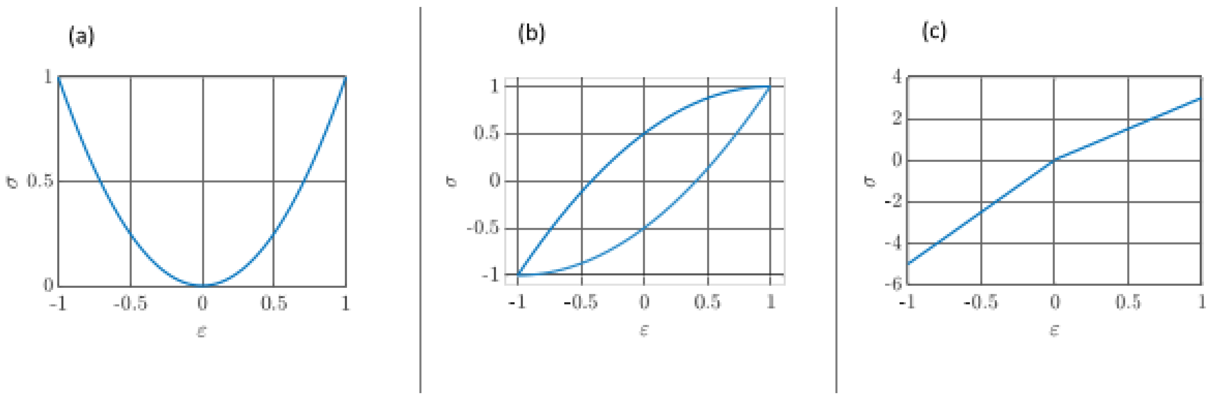
Figure 1.
Graphical representation of the stress(σ)–strain(ε) relation for a selection of scenarios characterized by non-linear mechanical behavior. A quadratic stress relation (a) is typical for classical nonlinearity. This type of nonlinearity is typically weakly present in all materials and becomes prominent for very large statically or vibration-induced stress levels. Hysteretic behavior (b) typically occurs when there is a frictional contact and short-range adhesion. Along with features of polygonal behavior (c), which is characteristic of delaminations in which the two limbs are less stiff to open by pulling than to close by pressing, hysteretic behavior can be expected for the hammer impact-induced delamination in the CFRP sample under investigation in this work.
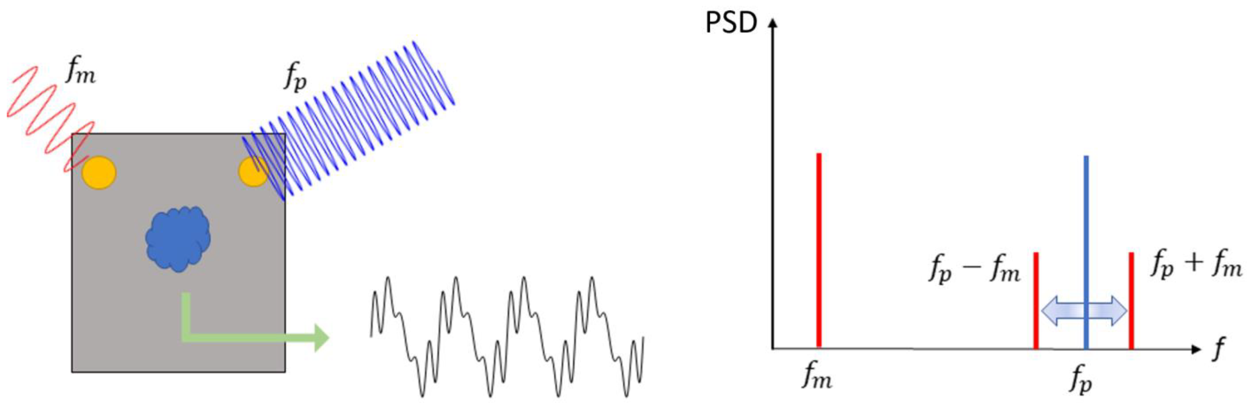
Figure 2.
Left: Schematic representation of acoustic frequency mixing. Left: two piezoelectric transducers (orange disks) force two respective sinusoidal vibrations in a plate to be tested. The first, low-frequency (), high-amplitude “pump” vibration is so strong that it dynamically modulates the mechanical response at the weak defect location (not elsewhere). The second, high-frequency () “probe” vibration with moderate amplitude is affected by this modulation. Right: At the defect location, due to the non-linear mechanical response of the medium, sum, and difference frequencies are generated, resulting in sidelobes left and right around the probe frequency (at frequencies fp − fm and fp + fm) in the power spectral density.
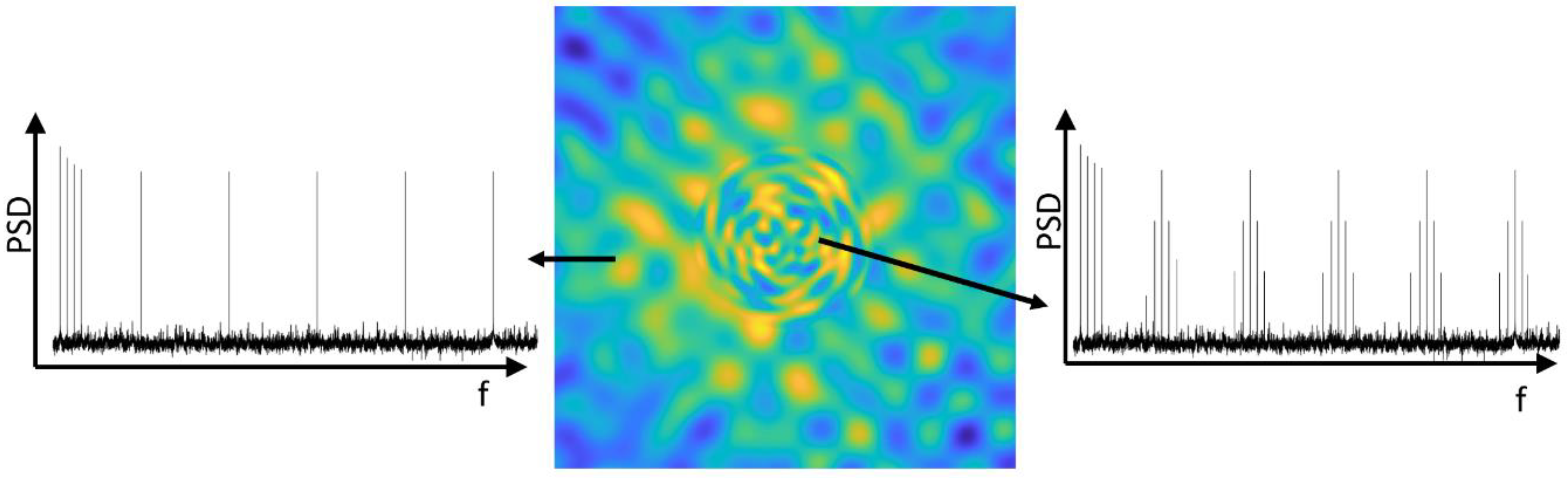
Figure 3.
Middle: Simulated displacement pattern in a plate excited by a low-frequency pumping wave and a series of harmonic probe frequency components characterized by a comb spectrum (frequencies nfcomb,0, n = 1..5). The blue–green chessboard pattern is representative of the standing waves set up by the probe vibrations. The larger displacements in the central region are caused by the pump vibration. The circular complex vibration behavior in the middle of the central region indicates nonlinear mixing between the pump vibration and the probing vibrations. Left: PSD in an intact part of the plate: only the pump vibration and its harmonics (resulting from classical mechanical nonlinearity) are present. Right: PSD in the middle of the central region, which is affected by defect-induced mechanical nonlinearity: in addition to the vibration components that are generated by the pump and probe transducers, mixing components are present in the form of side lobes around the probe comb frequencies, at frequencies pfP ± mfM (p = 1..5, m = 1,2). In principle, higher-order sidebands are generated by cross-modulation. In the experiment here reported, their amplitude was not significant enough to be used for defect localization.
![Vibration 06 00049 g003]()
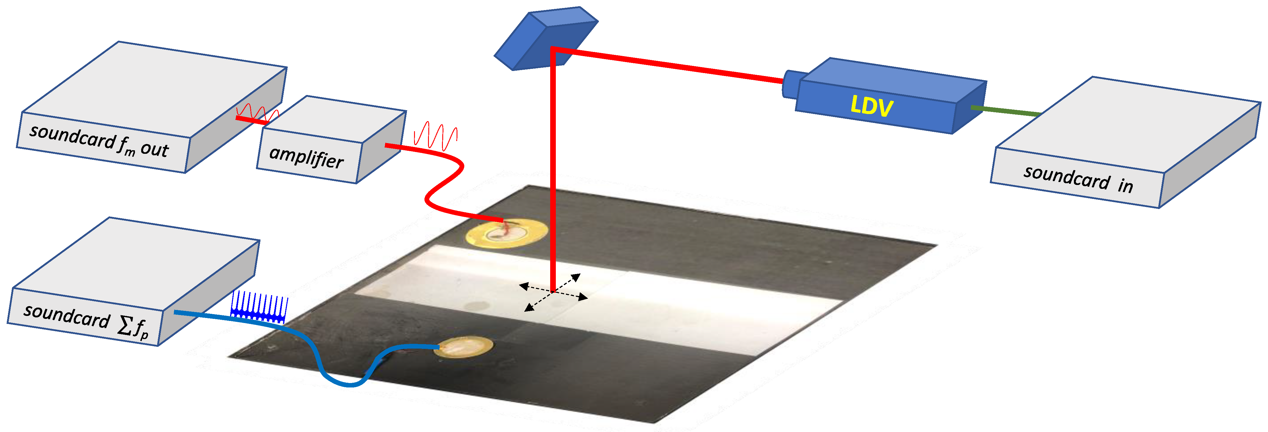
Figure 4.
Schematic set-up. The sample under study was a 1.7 mm thick, square, 300 × 300 m2 CFRP plate, consisting of 8 unidirectional plies overlapped in a 0–90° symmetric configuration. The barely visible impact damage was generated prior to vibrational testing by hitting the plate with a rubber hammer (contact surface 750 mm2). During vibrational testing, the plate was rigidly clamped at two edges (top and bottom in the photo). The area marked by gray reflective tape was scanned by the probe beam of a laser Doppler vibrometer (Polytec OFV-5000/sensor head OFV 505). The data were acquired using a commercial sound card (Roland Octa-Capture) that generated the excitation signal and recorded the resulting displacement. The modal excitation was amplified by a fixed gain amplifier (AA Lab Systems) and fed to a piezoelectric transducer that consisted of a PZT disk of 25 mm diameter (thickness 300 μm) glued on a 35 mm diameter brass plate (thickness 350 μm), which was in turn glued on the CFRP sample plate. For generating the probing waves, a second identical PZT–brass disk was glued on the CFRP sample plate.
![Vibration 06 00049 g004]()
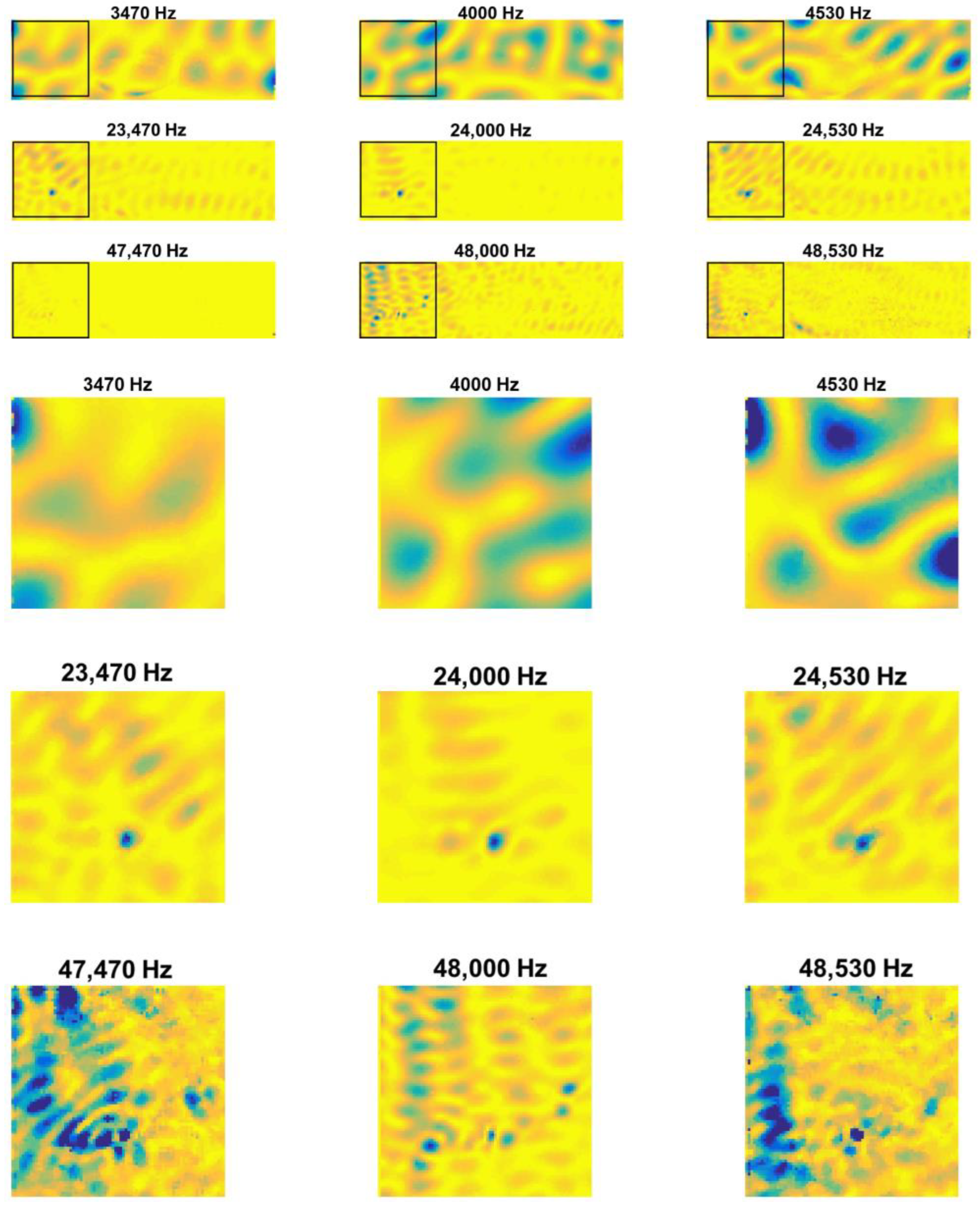
Figure 5.
Maps of the PSD of LDV scans. The velocity amplitude is represented in linear scale, blue corresponds to large velocity and yellow to lower velocity. The spatial maps of the PSD are shown at 3 selected comb probe frequencies, 4000 Hz, 24,000 Hz, and 48,000 Hz (
middle column), at the corresponding frequencies of left sideband, 3470 Hz, 23,470 Hz, and 47,470 Hz (
left column, and at the corresponding frequencies of the right sideband, 4530 Hz, 24,530 Hz, and 48,530 Hz (
right column). The color ranges are scaled between the minimum and maximum values of the shown region.
Top panel: along 85 × 290 mm
2 surface of retroreflective tape covered part of the CFRP sample in
Figure 3.
Bottom panel: zoom in on square 80 × 80 mm
2 region in the bottom left corner. The sidebands were caused by amplitude modulation of the probe vibration by a 530 Hz pump vibration (maximum amplitude across the inspected zone: 3.3 μm). The vibration amplitude is enhanced at the defect location (indicated by the arrow in the right middle map) in the maps obtained for the 6 highest frequencies. The defect contrast is very obvious around the 24,000 Hz comb frequency component. Interestingly, this defect feature shows up not only in the sideband maps but also at the probe comb frequencies 24,000 Hz and 48,000 Hz. Indicating that 24,000 Hz and 48,000 Hz are LDRs. The strain induced by the pump and probing waves was calculated to be about
, while for the probe wave, it was about
. The value of the measured strain is in line with values reported in the literature on similar experiments [
41,
48].
![Vibration 06 00049 g005]()
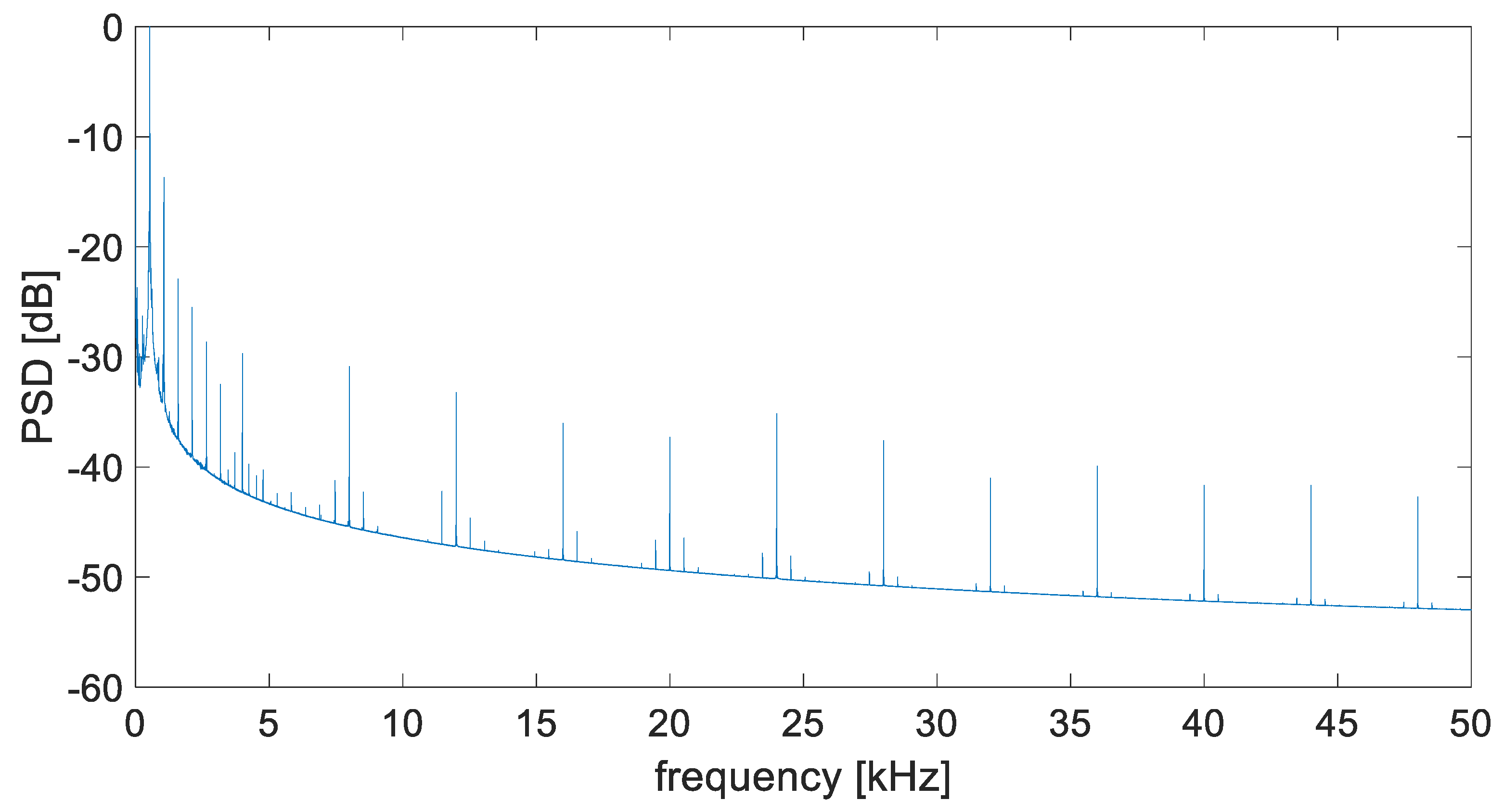
Figure 6.
Spectrum of the velocity amplitude at the defect location rescaled with respect to the pump amplitude. At lower frequencies, the harmonics of the pump vibration are visible. The comb frequencies are fp = pfP with fP = 4000 Hz (p = 1..12). The sideband amplitude is approximately 10 dB smaller than the corresponding comb component.
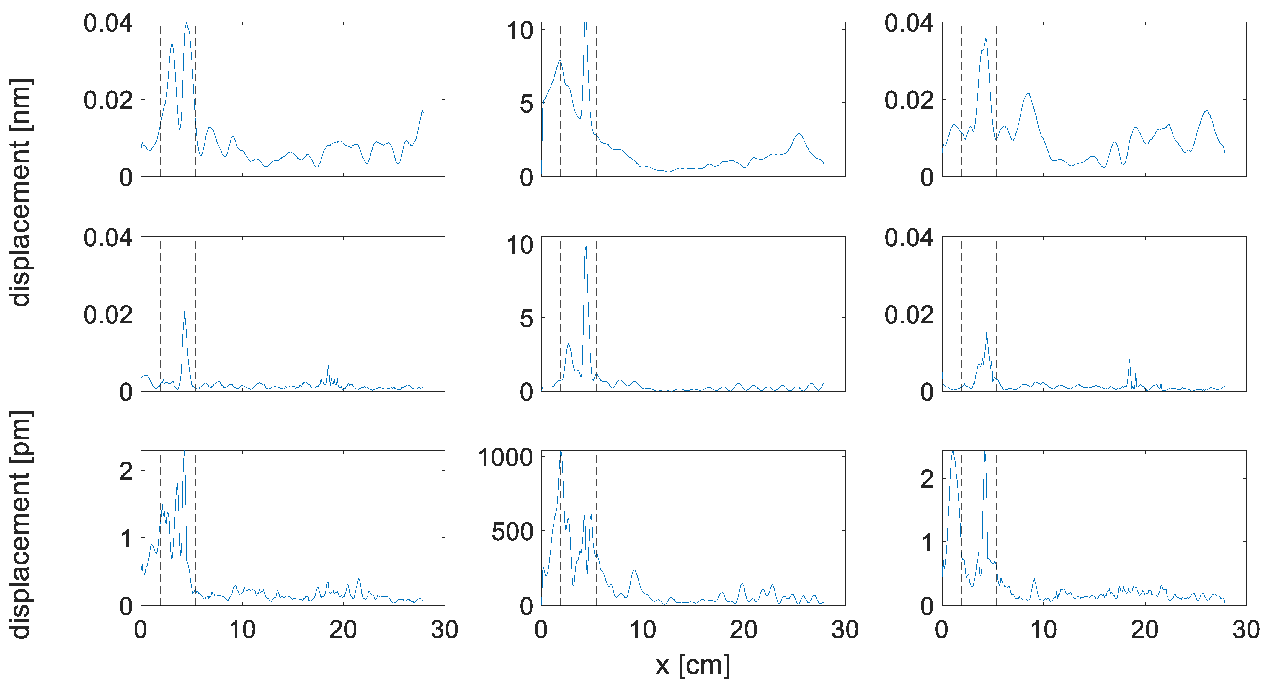
Figure 7.
Top: Cross-sections along the horizontal direction and through the defect of the LDV signal displacement amplitude maps in
Figure 4 for the 24,000 Hz probe frequency (
middle) and the two sidebands (
left: 23,470 Hz,
right: 24,530 Hz). The vertical dashed lines delimit the defect’s location as identified in
Figure 8, the RMS amplitude of all sidebands.
Middle: same as top, but here the RMS of all comb frequencies (
pfP = 4 kHz to 48 kHz and respective sidebands
pfP ±
fM) is depicted.
Bottom: displacement amplitude maps in
Figure 4 for the 48,000 Hz probe frequency (
middle) and the two sidebands (
left: 47,470 Hz,
right: 48,530 Hz). Note the vertical axis is in nm for the first two rows and pm for the last one, since the amplitude of the sidebands and of the comb is substantially smaller for the 48,000 Hz than for the 24,000 Hz and RMS case.
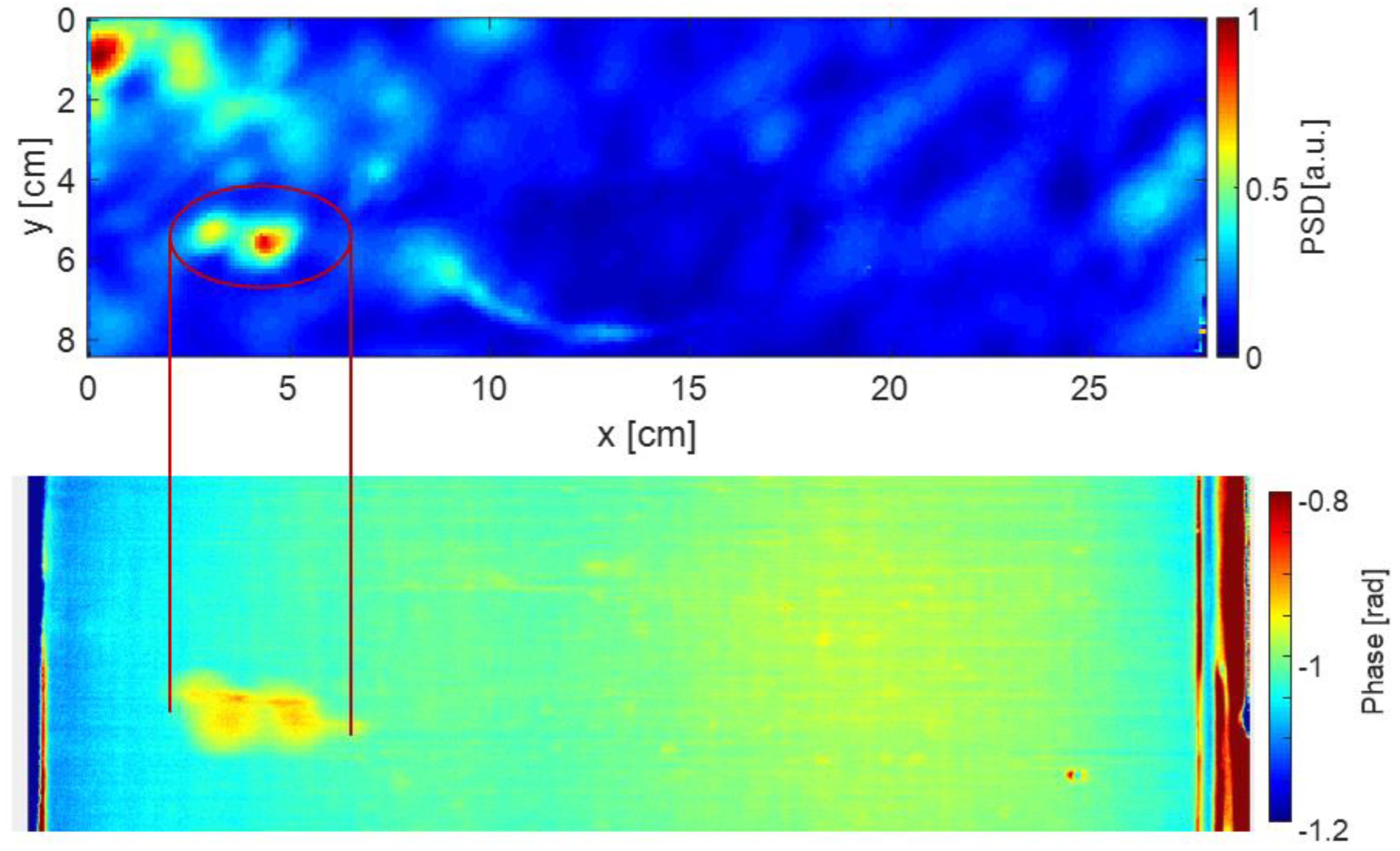
Figure 8.
Comparison between the image obtained by taking the RMS value across all satellite (top) and thermographic phase image (f = 0.3 Hz) obtained by pulsed photothermal excitation on the front side of the carbon fiber-reinforced sample plate with the flash lamp alimented with an electrical pulse of 3 kJ and 2 ms duration. The heating transient was recorded from the opposite side of the sample by an infrared camera (FLIR X8500SC (Teledyne FLIR LLC, Wilsonville, OR, USA) ). Signs of the defect are consistently indicated in both the vibrational and thermographic images, albeit with significantly better contrast in the latter. In the top left corner, an additional signature of cross-modulation is present. This is due to a locally improper clamping at the edge, caused by vibrational friction at a ridge at the edge of the plate. The surface scanned by the LDV is slightly smaller than the surface imaged by the IR camera because of the clamping present in the sideband imaging experiments. The defect is inside the red ellipse in the RMS image (top) and its left and right boundaries are projected in the IR image (bottom) by the red markings.
![Vibration 06 00049 g008]()
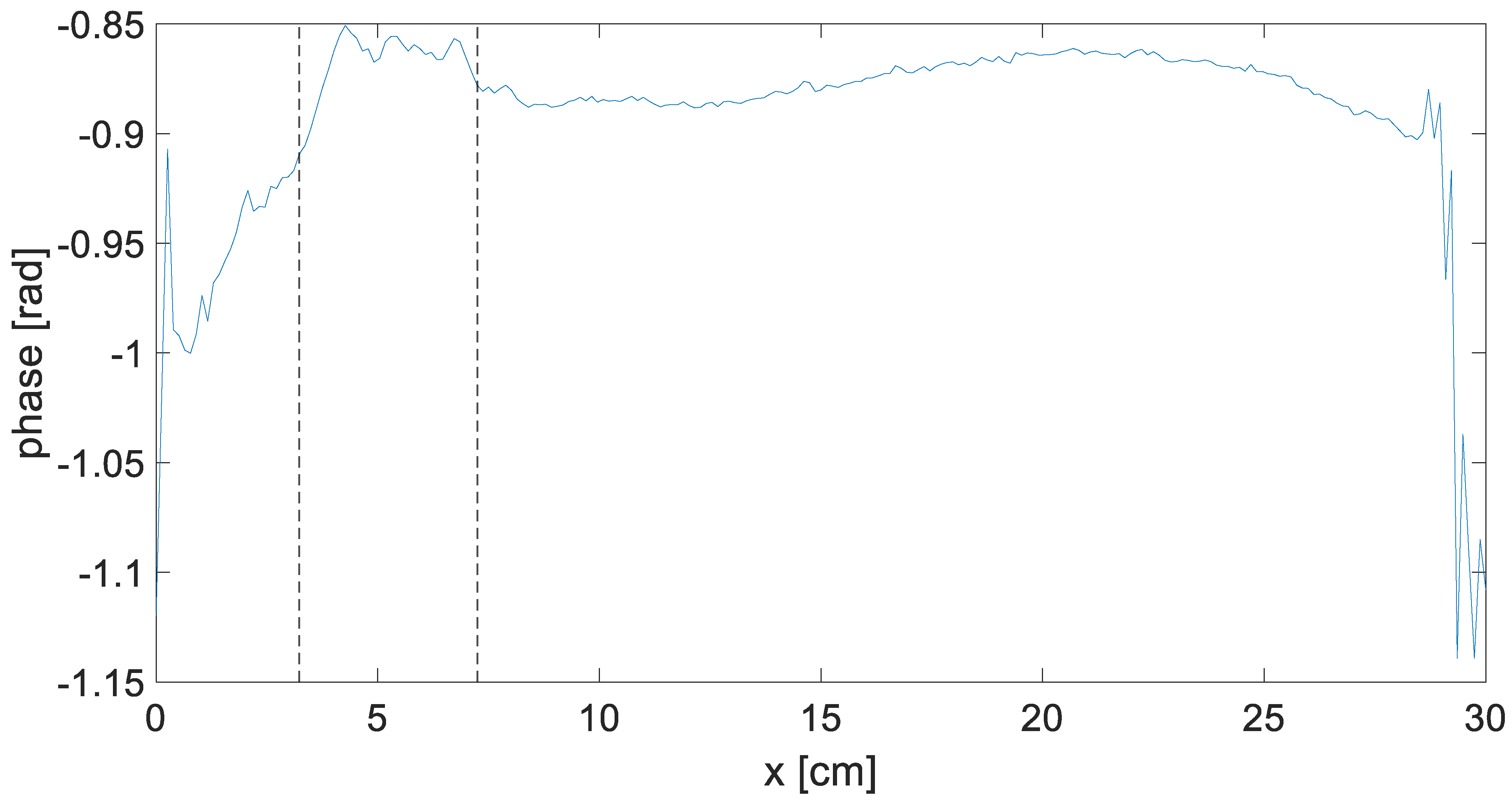
Figure 9.
Cross-section through the defect region of the infrared phase image in
Figure 5, averaged over a strip of 4 cm wide in the horizontal (x) direction. The vertical dotted lines mark the defect boundaries along the x-axis.
Figure 9.
Cross-section through the defect region of the infrared phase image in
Figure 5, averaged over a strip of 4 cm wide in the horizontal (x) direction. The vertical dotted lines mark the defect boundaries along the x-axis.
Figure 10.
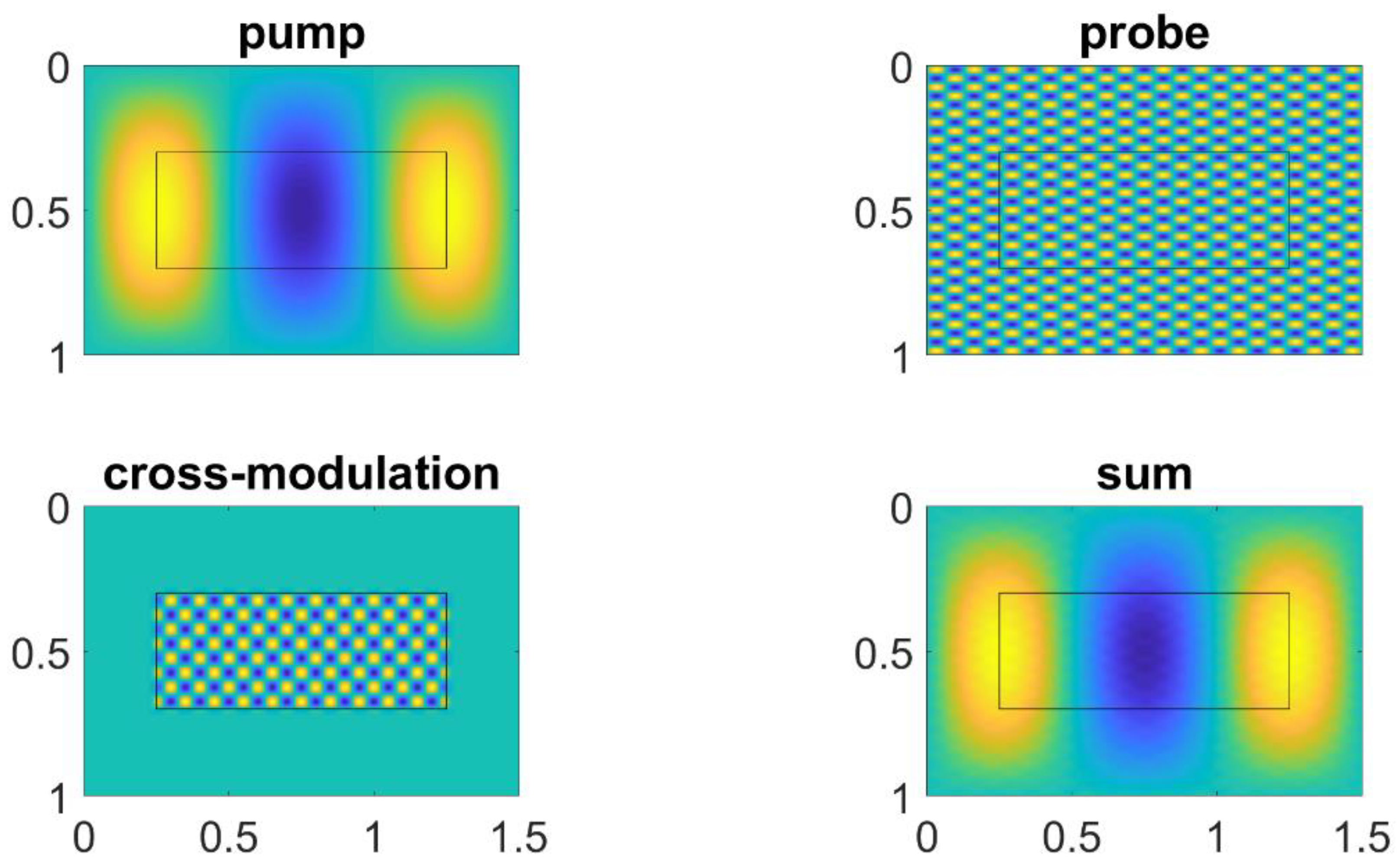
Simulation of the different vibration patterns involved in a cross-modulation experiment shown isolated. The border of the defect is depicted by the black rectangle in the center of the image. Top left, pump component. Top right, probe component. Bottom left, sideband component. The sideband vibration is only happening at the defect location. Bottom right, sum of all the displacement patterns. Due to the big difference in amplitude, the pump mode mostly determines the displacement pattern in the sum figure.
Figure 10.
Simulation of the different vibration patterns involved in a cross-modulation experiment shown isolated. The border of the defect is depicted by the black rectangle in the center of the image. Top left, pump component. Top right, probe component. Bottom left, sideband component. The sideband vibration is only happening at the defect location. Bottom right, sum of all the displacement patterns. Due to the big difference in amplitude, the pump mode mostly determines the displacement pattern in the sum figure.
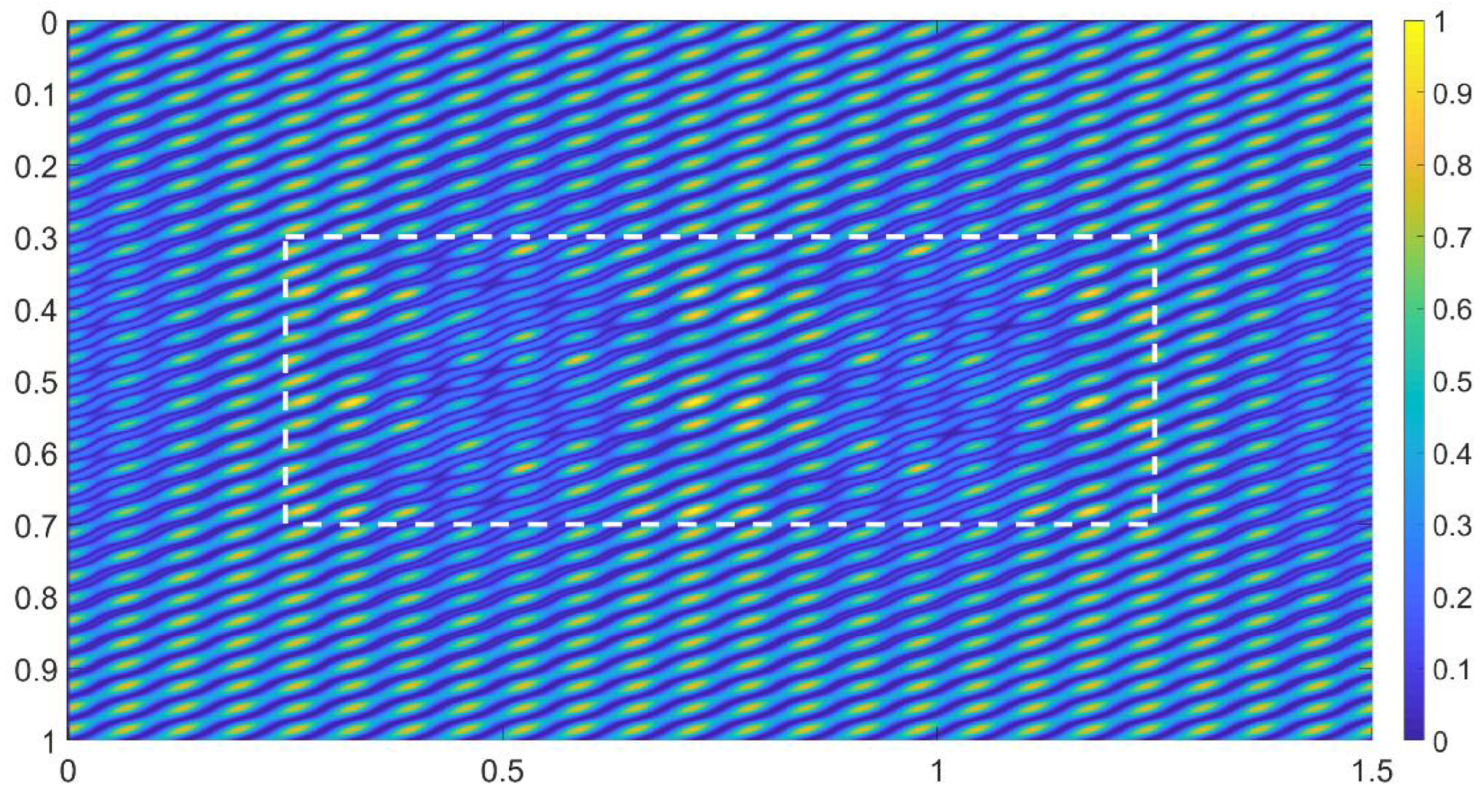
Figure 11.
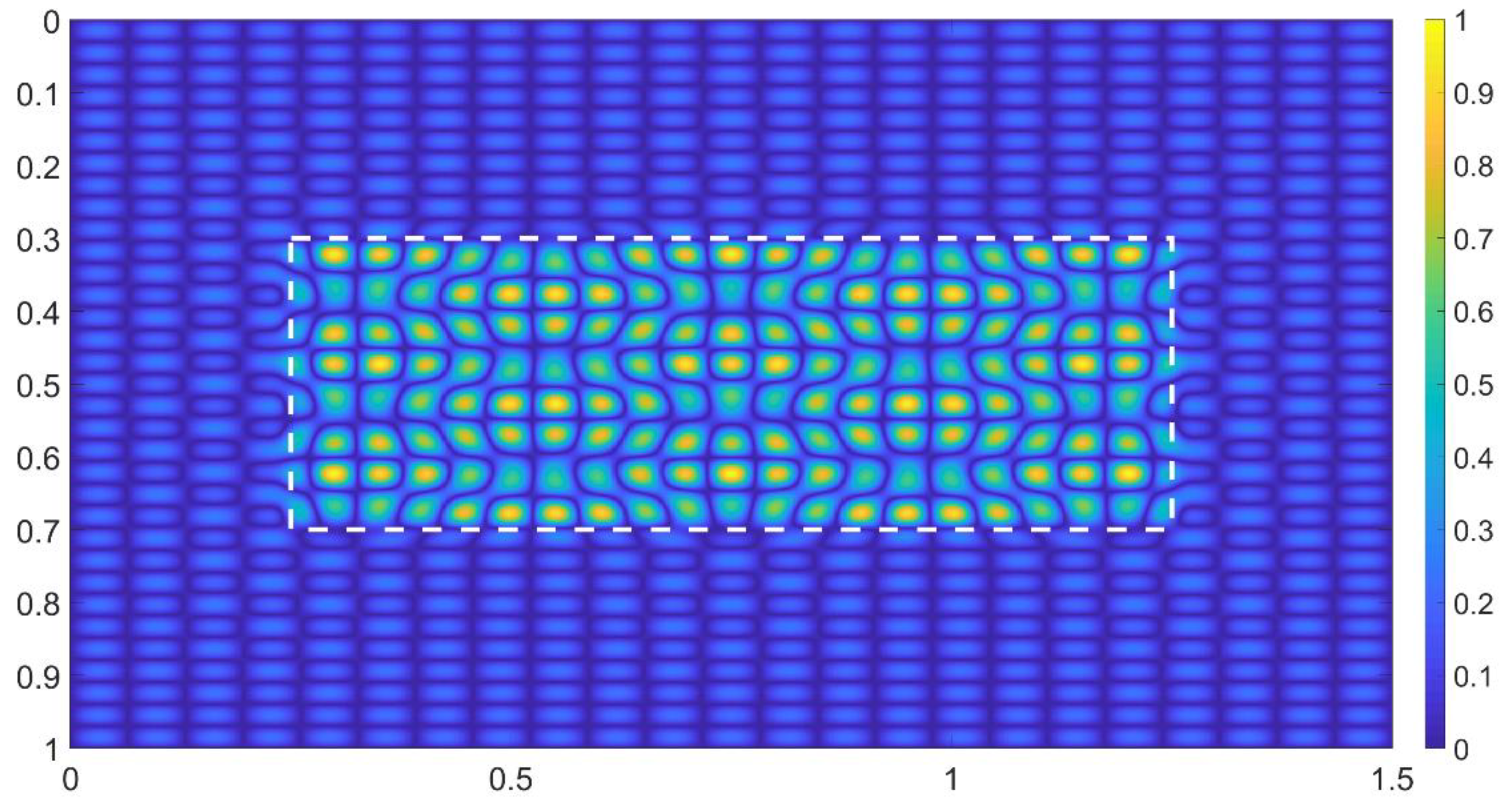
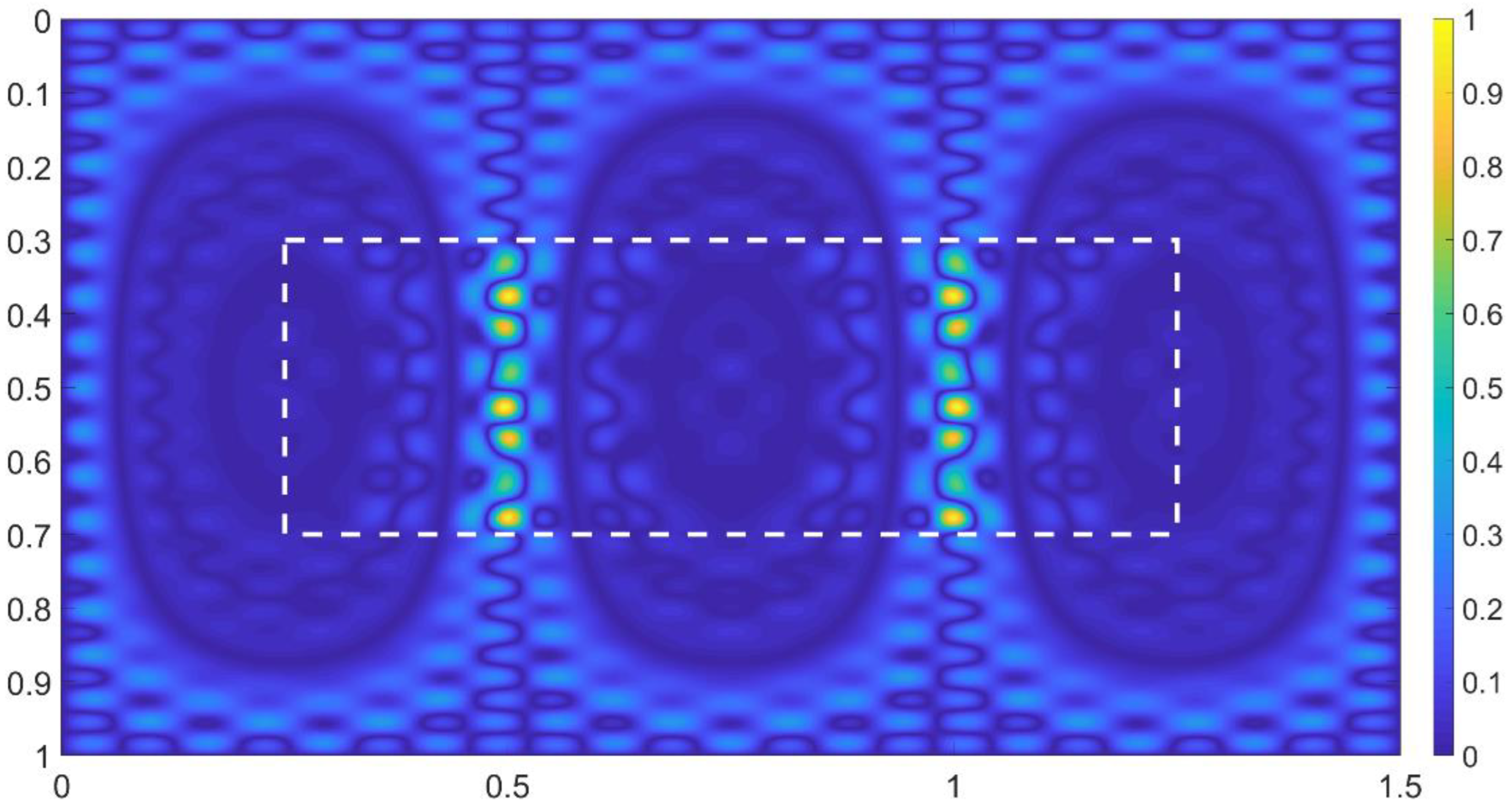
Simulated map of the sinusoidal interferometer signal component at a frequency of vibration of interest (23,470 Hz, left sidelobe) of a plate subject to a superposition of a 530 Hz large (δpump = 3.3 μm amplitude) sinusoidal vibration with wavelength of about 1 unit and a 4000 Hz small (δprobe10 nm amplitude) sinusoidal vibration with wavelength of about 0.13 units across the whole surface. A small 23,470 Hz (δdefect = 50 pm amplitude) sinusoidal vibration, mimicking a mechanical nonlinearity-induced vibration of interest, is superposed on the other two vibrations in the white rectangle. Ideally, one would expect to see a large contrast between the rectangular region in which the vibration of interest is present, and the remainder of the plate. In contrast, the map of the 23,470 Hz interferometer signal amplitude is not at all determined by the vibration of interest, but by the optical nonlinearity-induced mixing between the 530 Hz vibration and the 24,000 Hz probe vibration, which yields a difference frequency signal component of 23,470 Hz across the whole plate, with an amplitude (intensity modulation depth of the order of 1) much larger than the one resulting from the vibration of interest (intensity modulation of the order of 10−4). Light intensity is normalized to its maximum.
Figure 11.
Simulated map of the sinusoidal interferometer signal component at a frequency of vibration of interest (23,470 Hz, left sidelobe) of a plate subject to a superposition of a 530 Hz large (δpump = 3.3 μm amplitude) sinusoidal vibration with wavelength of about 1 unit and a 4000 Hz small (δprobe10 nm amplitude) sinusoidal vibration with wavelength of about 0.13 units across the whole surface. A small 23,470 Hz (δdefect = 50 pm amplitude) sinusoidal vibration, mimicking a mechanical nonlinearity-induced vibration of interest, is superposed on the other two vibrations in the white rectangle. Ideally, one would expect to see a large contrast between the rectangular region in which the vibration of interest is present, and the remainder of the plate. In contrast, the map of the 23,470 Hz interferometer signal amplitude is not at all determined by the vibration of interest, but by the optical nonlinearity-induced mixing between the 530 Hz vibration and the 24,000 Hz probe vibration, which yields a difference frequency signal component of 23,470 Hz across the whole plate, with an amplitude (intensity modulation depth of the order of 1) much larger than the one resulting from the vibration of interest (intensity modulation of the order of 10−4). Light intensity is normalized to its maximum.
![Vibration 06 00049 g011]()
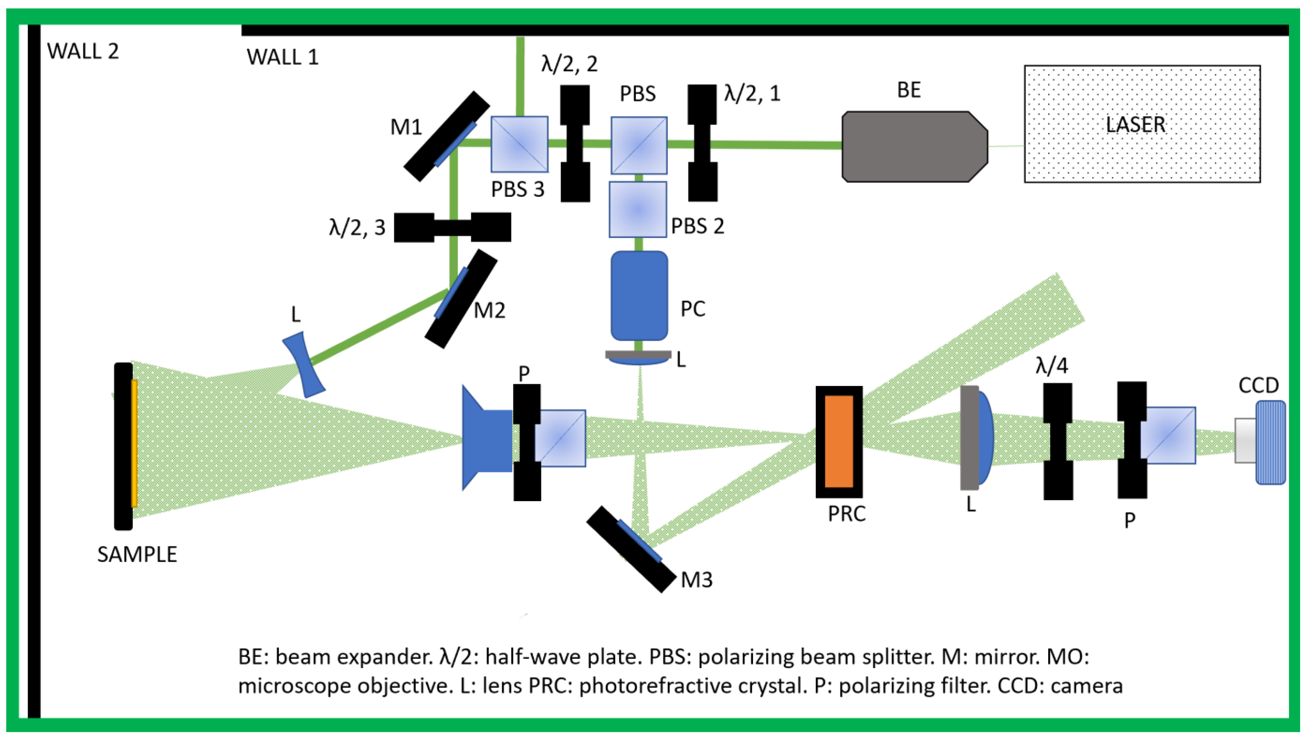
Figure 12.
Schematic setup of a photorefractive interferometer in bandpass mode. The Pockels cell (PC) is driven by a sinusoidal voltage a frequency fP of interest from a high voltage amplifier that in turn is driven by a function generator. In this scheme, the CCD delivers vibrometric images varying at frequency Ω = fvibration − fP with a bandpass-type response with center frequency fP and bandwidth fBW = 1/(2πτ) = 106 Hz, with τ = 1.5 s the response time of the photorefractive crystal (PRC). Half wave (λ/2) plates 1,2,3, respectively, control the fraction of the laser power that is sent into the reference, the power of the sample beam, and the polarization of the sample beam when entering the PRC after collection by the objective O and the rotatable polarizing beam splitter P. The objective O together with the lens L make a sharp image of the sample on the CCD. Lens L also ensures a sharp image of the reference light diffracted by the PRC, which contains the spatially resolved information about the vibration, onto the CCD. Rejection of sample beam light through the PRC, while passing the part of the (anisotropically) diffracted reference beam that is perpendicularly polarized to the sample beam is aimed for by insertion of the rotatable polarizing beam splitter P. The quarter wave (λ/4) plate helps to reject the part of the sample beam that is optically rotated in the PRC.
![Vibration 06 00049 g012]()
Figure 13.
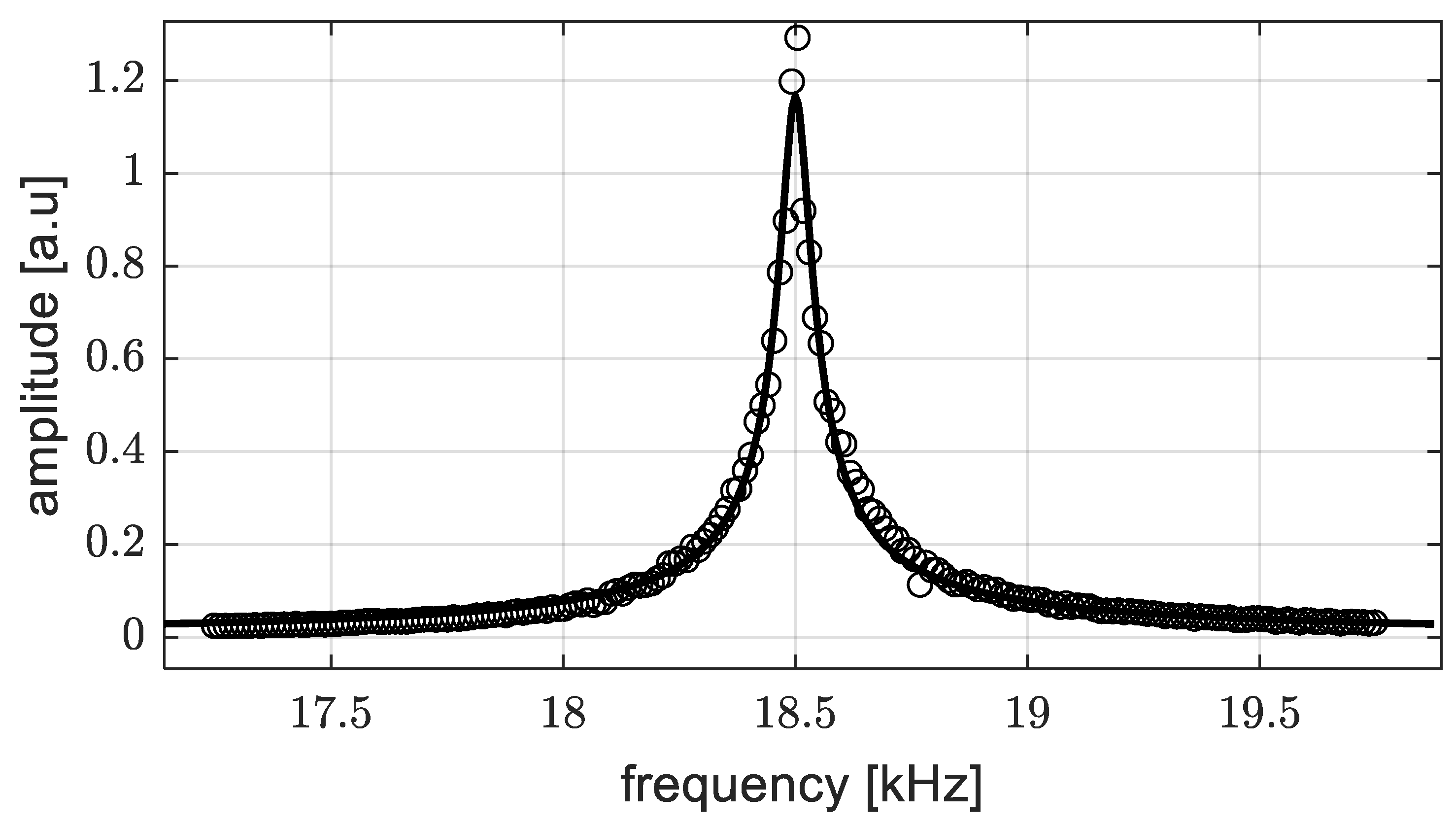
Experimentally determined characteristic bandpass spectrum of the PRI-BP for a Pockels cell phase modulation frequency swept from 17 to 20 kHz. A Thorlabs DET36A/M photodetector was used to detect the diffracted reference beam and a Stanford Research lock-in amplifier SR830 was used to determine its intensity modulation amplitude.
Figure 13.
Experimentally determined characteristic bandpass spectrum of the PRI-BP for a Pockels cell phase modulation frequency swept from 17 to 20 kHz. A Thorlabs DET36A/M photodetector was used to detect the diffracted reference beam and a Stanford Research lock-in amplifier SR830 was used to determine its intensity modulation amplitude.
Figure 14.
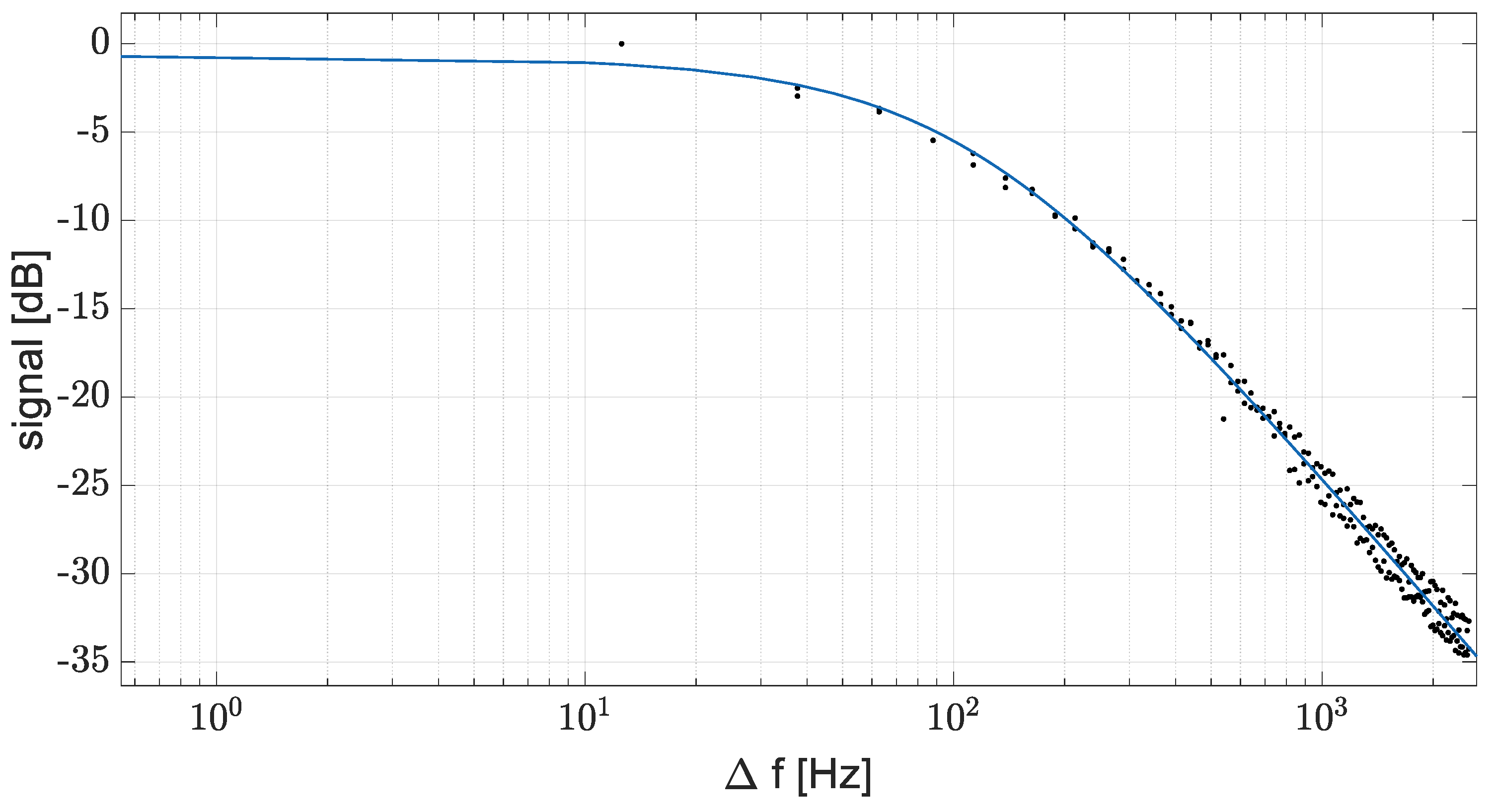
Plot of the bandpass filtering of the PRI in logarithmic scale.
indicates the difference between the frequency of vibration in the sample (18.5 kHz) and the frequency of the phase modulation in the reference beam. This figure is a rearrangement of
Figure 13. The attenuation is about 20 dB per decade as per a conventional electrical 1st order bandpass filter.
Figure 14.
Plot of the bandpass filtering of the PRI in logarithmic scale.
indicates the difference between the frequency of vibration in the sample (18.5 kHz) and the frequency of the phase modulation in the reference beam. This figure is a rearrangement of
Figure 13. The attenuation is about 20 dB per decade as per a conventional electrical 1st order bandpass filter.
Figure 15.
Illustrated map of the sinusoidal PRI-BP signal component locking on a sideband vibration in presence of a pump and a probe vibration as in
Figure 10, i.e., at a frequency of vibration of interest (23,470 Hz) of a plate subject to a superposition of a 530 Hz large (δ
pump = 100 nm amplitude) sinusoidal vibration with wavelength of about 1 units and a 24,000 Hz small (δ
probe= 10 nm amplitude) sinusoidal vibration with wavelength of about 0.13 units across the whole surface. A small 23,470 Hz (δ
defect = 0.5 nm amplitude) sinusoidal vibration, mimicking a mechanical nonlinearity-induced vibration of interest, is superposed on the other two vibrations in the white rectangle. Thanks to the strong suppression of vibrational components other than the vibration of interest, the image clearly shows the presence of the vibration of interest in the rectangular “defect region”, and it is not affected by the presence of the two other vibrations. The values of the pump and probe amplitude are much smaller than what are used in the LDV experiments of the section above. This simulation illustrates the frequency selective imaging capability of the PRI in ideal setting. When the pump vibration pattern has large differences between the regions with maximum displacement (antinodes) and those with minimum displacement (nodes) a masking term modulates the resulting light amplitude, as illustrated in
Figure 16.
![Vibration 06 00049 g015]()
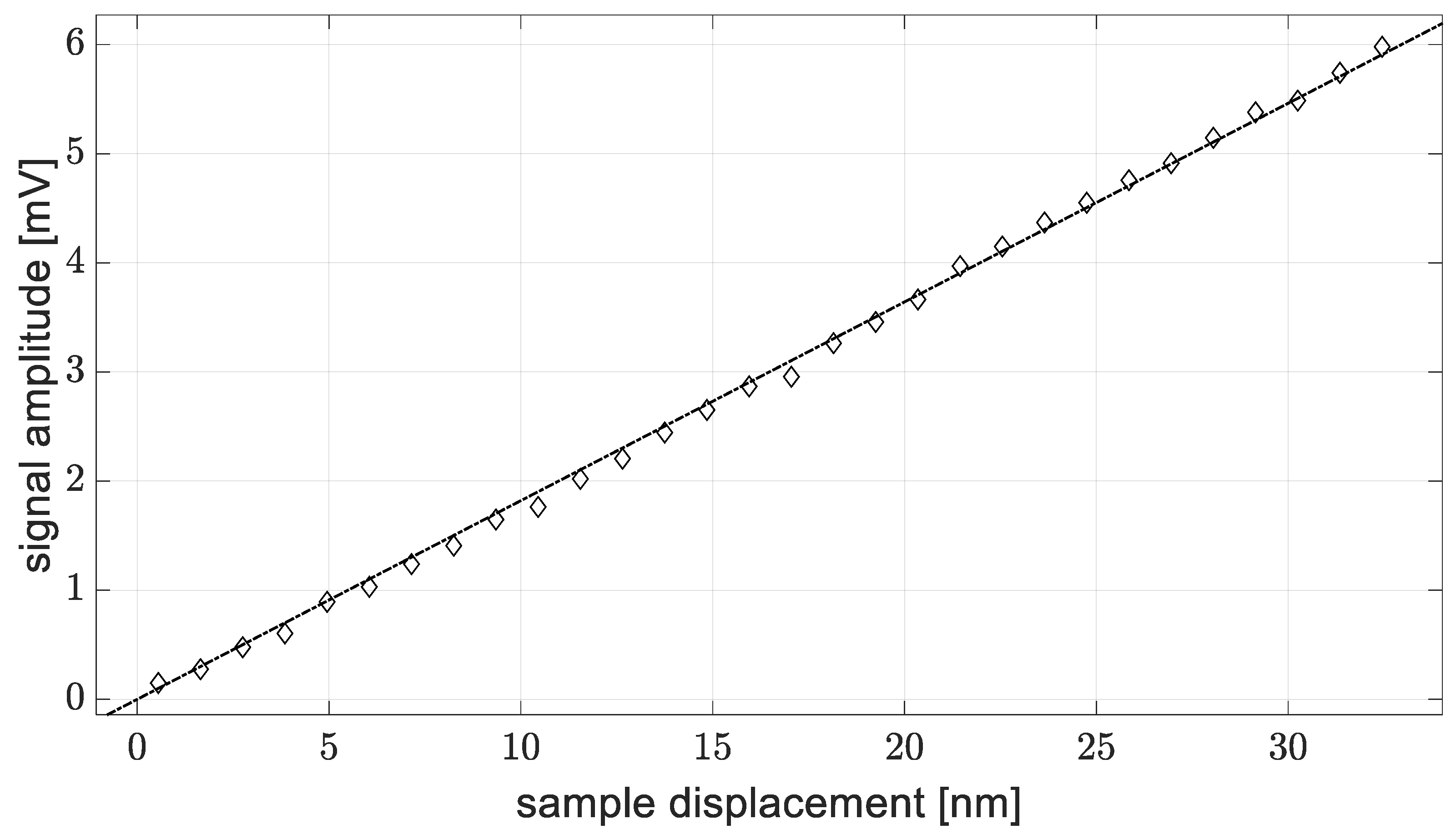
Figure 17.
Amplitude of the PRI-BP detected signal versus amplitude of a sinusoidal sample displacement. The sample was a sinusoidally vibrating piezoelectric disk actuator consisting of a PZT disk of 300 μm thickness and 35 mm diameter glued on a 350 μm thick and 50 mm diameter brass disk that in turn was clamped in a 40 mm diameter rigid ring. The light beam intensities were 354 mW/cm2 for the reference beam and 0.42 mW/cm2 for the collected part of the sample beam (beam power values measured in front of the PRC surface using a Thorlabs PM100D power meter with detector S132C (Newton, NJ, USA)).
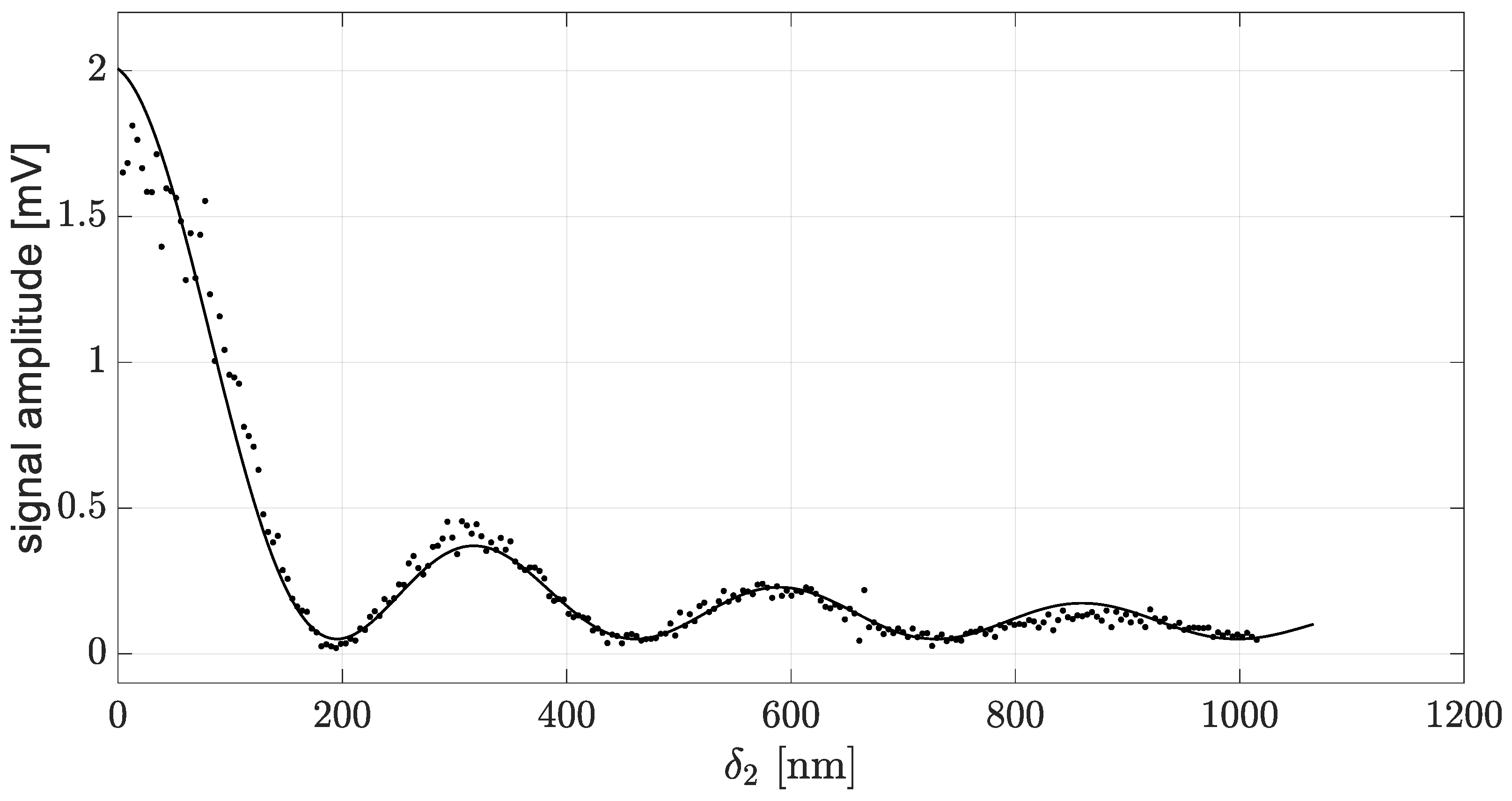
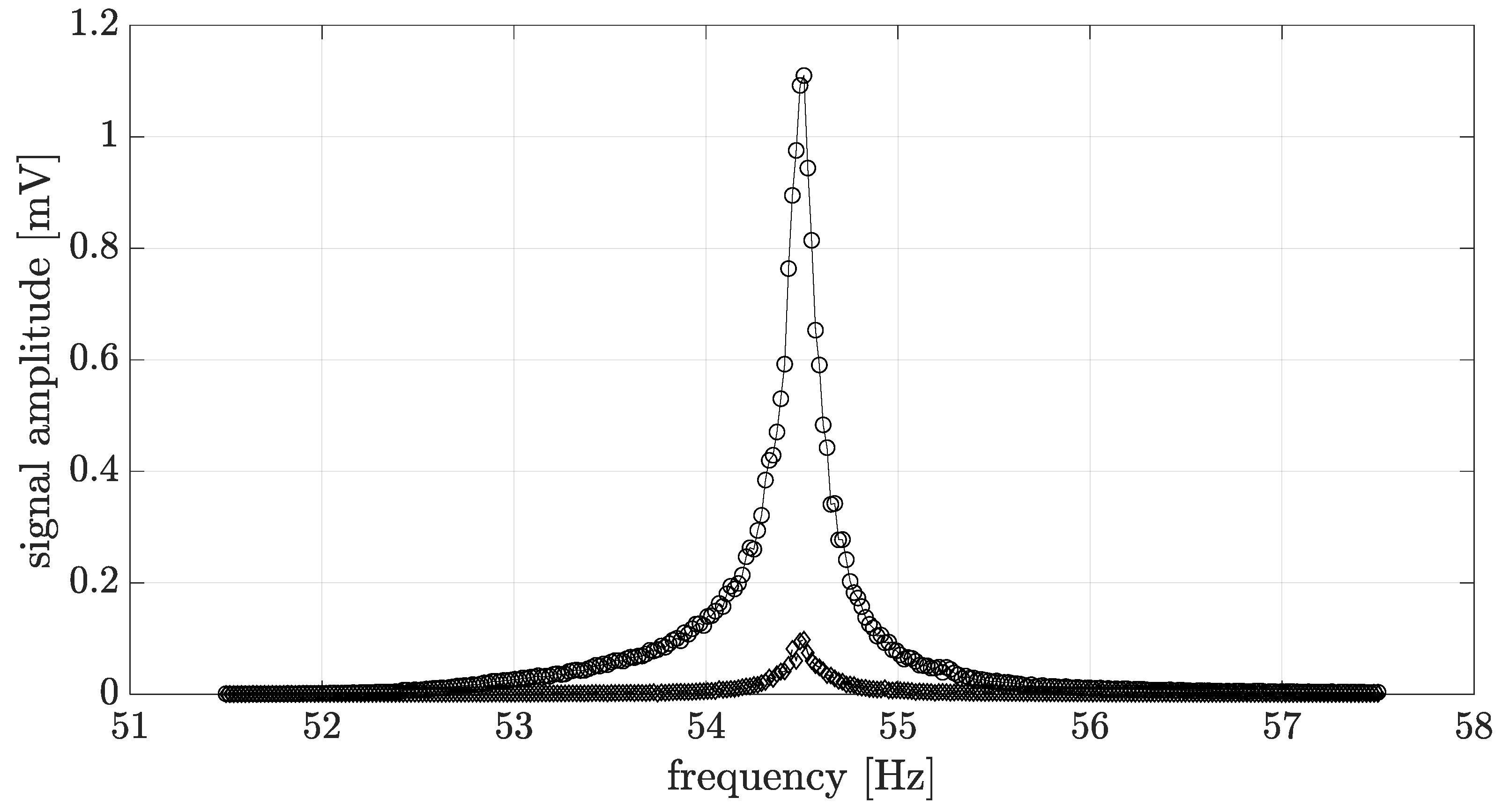
Figure 18.
Experimentally determined characteristic bandpass spectrum in two scenarios, in which, (i) the sample PZT is vibrating a single vibration frequency at 54.5 kHz (amplitude δ1 = 44 nm) (circle markers), (ii) a second, large vibration component at 57 kHz was added, with an amplitude of δ2 = 380 nm resulting in an unwanted suppression of the signal of interest with a factor with
, diamond markers. The Pockels cell optical phase modulation was swept in both cases from 50.5 kHz to 57.5 kHz. The experimental approach used to obtain these data was analogous to the one that was used to obtain the data in
Figure 13.
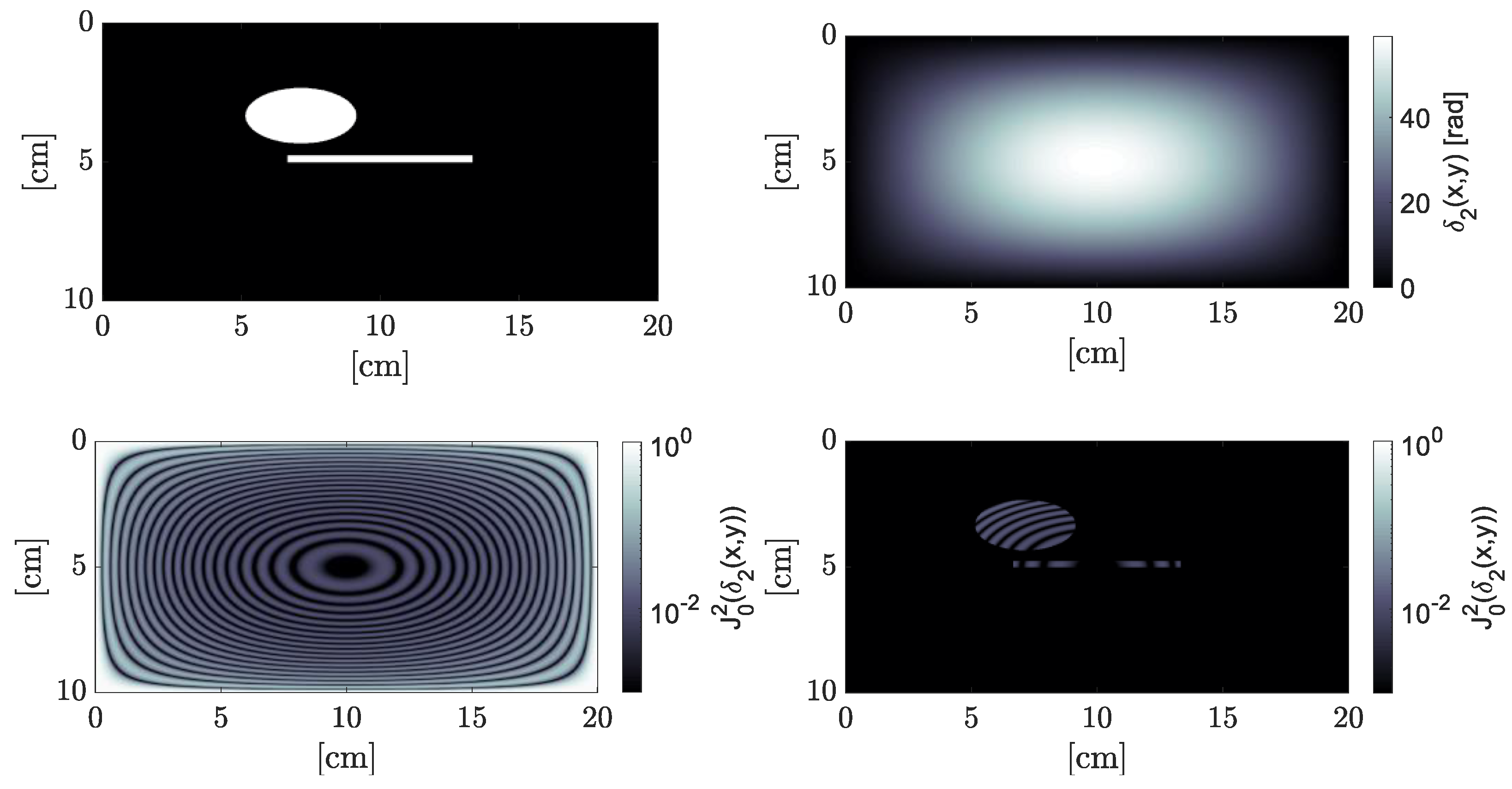
Figure 19.
Illustration of how the masking would affect the visualization of an elliptic and a linear defect (
top left) generating acoustic cross modulation. Although the pump and probe vibrations can be efficiently rejected, the large amplitude (here: 5 μm) of the pump vibration (displacement map:
top right) results in fringes in the vibration map, of which the spatial structure is not related to the vibration of interest but to the pump vibration (
bottom left). The effect of the masking is a reduced reliability in the definition of the defect. The defect may appear as a set of multiple small features (
bottom right) By varying the pump amplitude and taking the average of the images, the fringe structure can be spatially smeared out, resulting in the map in panel
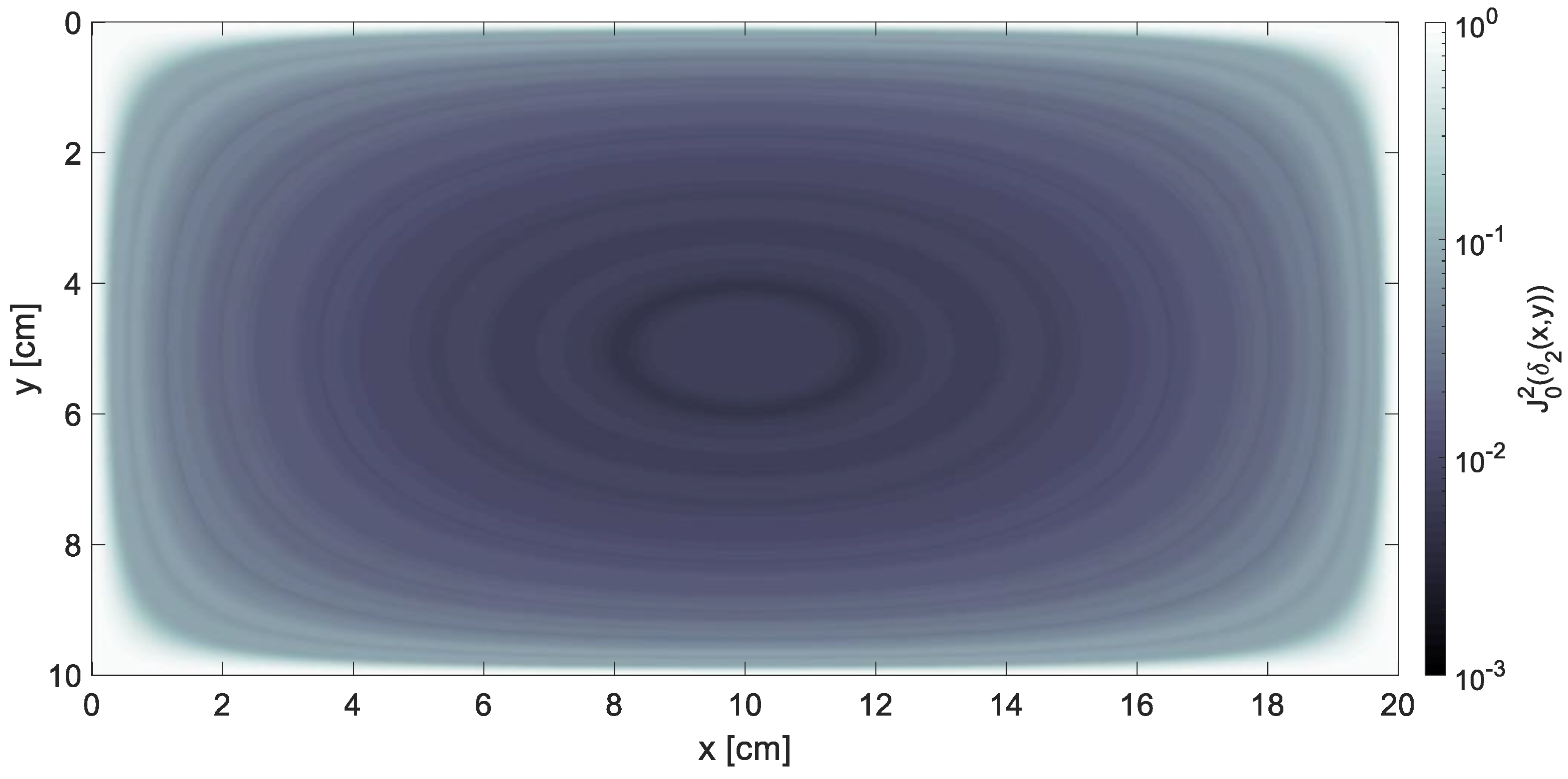
Figure 20, which is almost monotonic.
Figure 19.
Illustration of how the masking would affect the visualization of an elliptic and a linear defect (
top left) generating acoustic cross modulation. Although the pump and probe vibrations can be efficiently rejected, the large amplitude (here: 5 μm) of the pump vibration (displacement map:
top right) results in fringes in the vibration map, of which the spatial structure is not related to the vibration of interest but to the pump vibration (
bottom left). The effect of the masking is a reduced reliability in the definition of the defect. The defect may appear as a set of multiple small features (
bottom right) By varying the pump amplitude and taking the average of the images, the fringe structure can be spatially smeared out, resulting in the map in panel
Figure 20, which is almost monotonic.
Table 1.
Overview of the minimum detectable displacement of the LDV setup and the PRI-BP setup in different configurations.
Table 1.
Overview of the minimum detectable displacement of the LDV setup and the PRI-BP setup in different configurations.
| Minimum Detectable Displacement/Noise Level | pmW1/2/Hz1/2 | pm/Hz1/2 |
|---|
| PRI-BP point detection theoretical value | 32 × 10−6 | 0.14@P = 50 nW |
| PRI-BP point detection experimental value | 22 × 10−3 | 10@P = 10−5 nW/pixel |
| PRI-BP full-field experimental value | 300 × 10−6 | 3000@P = 10−5 nW/pixel |

 ,
, 


