3.1. Results of the Statistical Evaluation of Sensing Characteristics
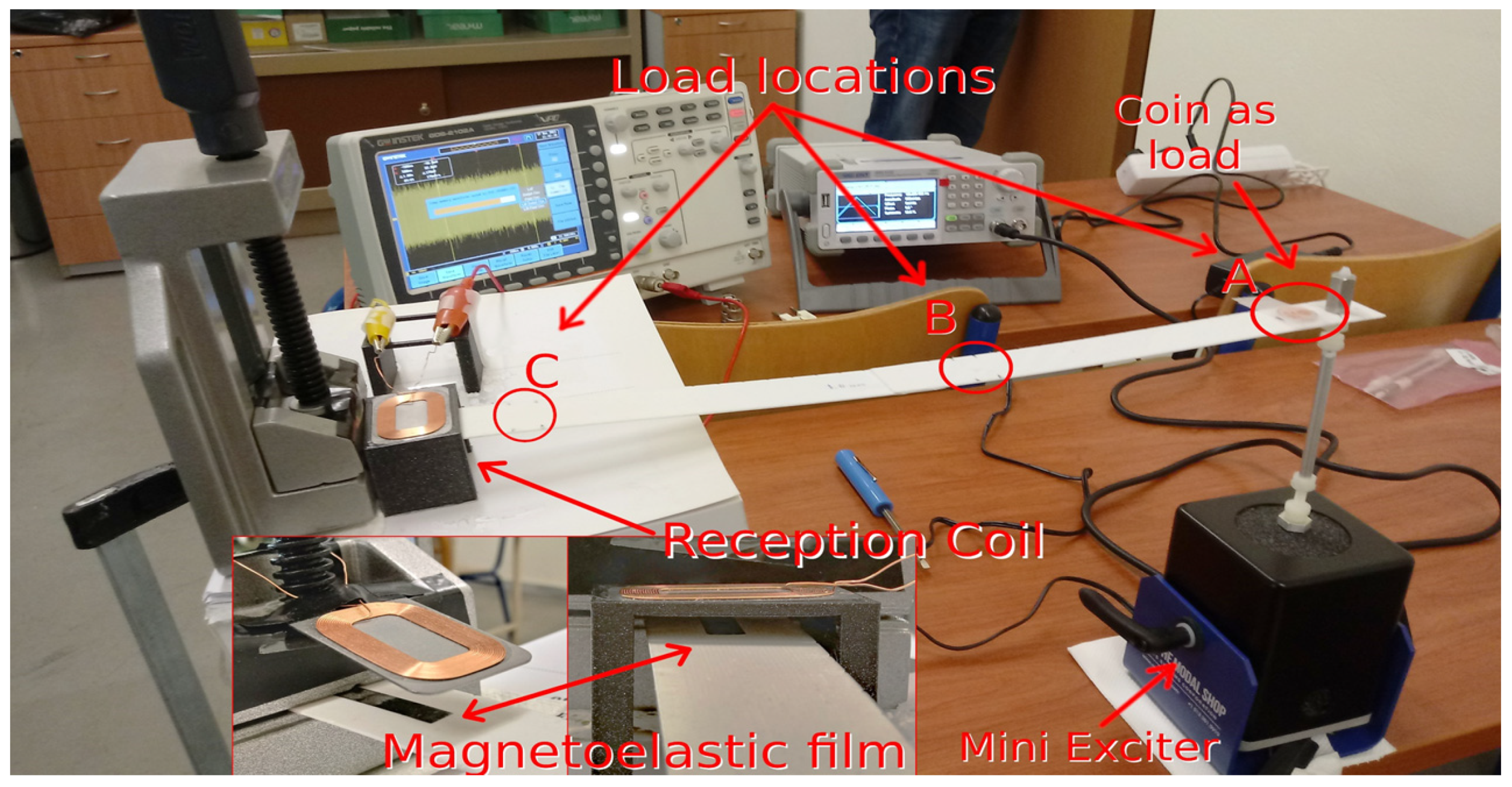
The testing procedure involved six experiments for each excitation level, as presented in
Table 2. The reception coil was placed at a distance of 5 mm above the ribbon, following the relevant testing performed in [
24], to define an optimal value for that distance. As seen in
Table 2, the beam was excited with frequencies starting at 10 Hz for the first series of six experiments and finishing at 160 Hz for the last series. In general, at each test series, the excitation level increased by 15 Hz with respect to the previous one. The only exception to this rule regarded the test series with the beam excited at 25 Hz, which presented very similar results to those obtained when the beam was under an excitation of 10 Hz (see also the relevant comment later on) and was therefore omitted. Note also that a test series of six experiments with the beam at rest, namely, series zero, was included for comparison purposes. The voltage signals were recorded and examined with respect to their frequency content. In
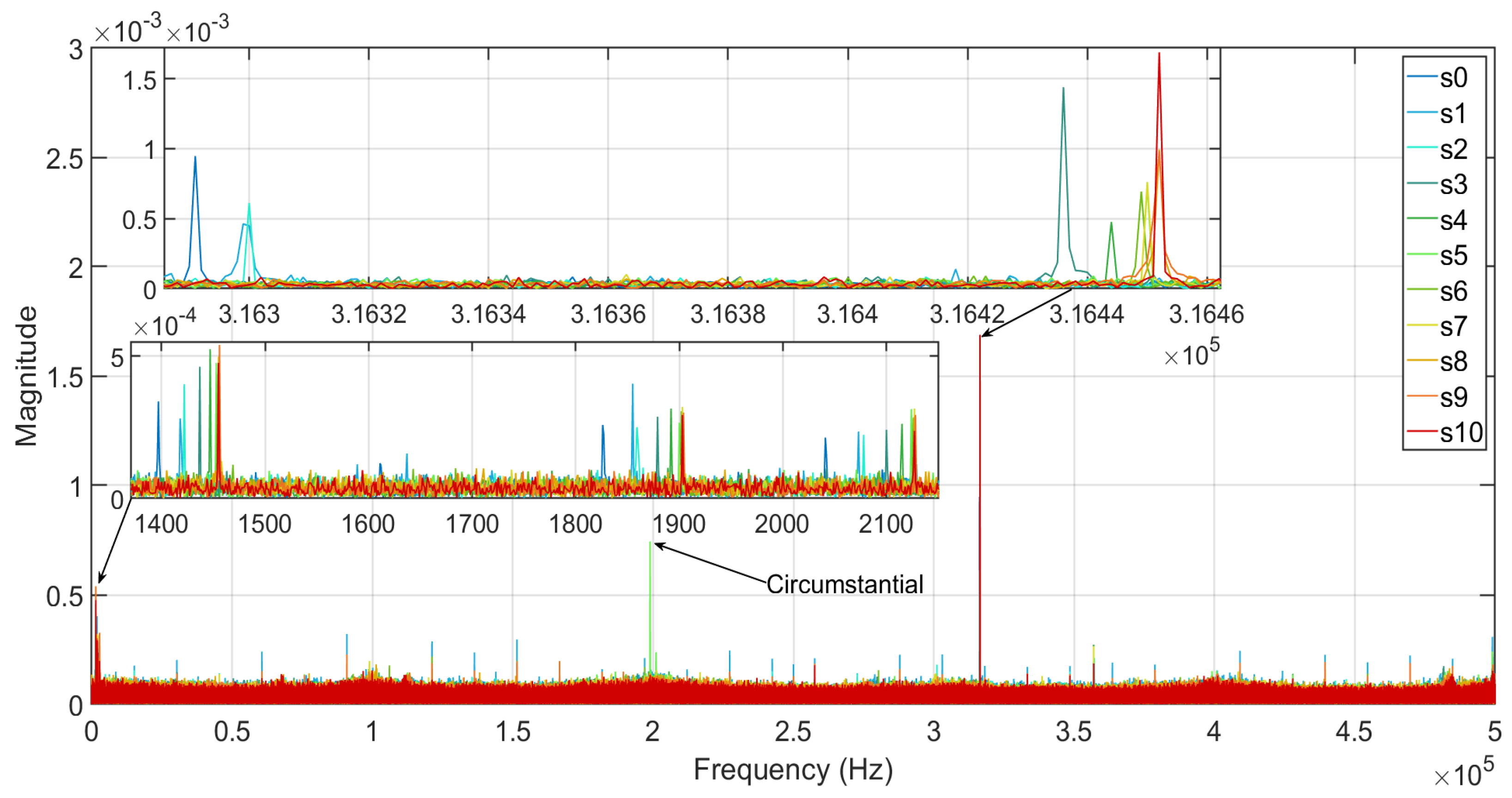
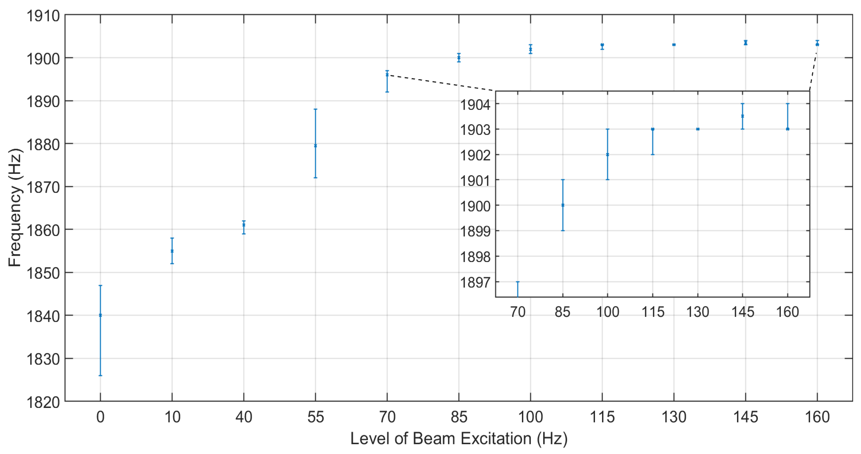
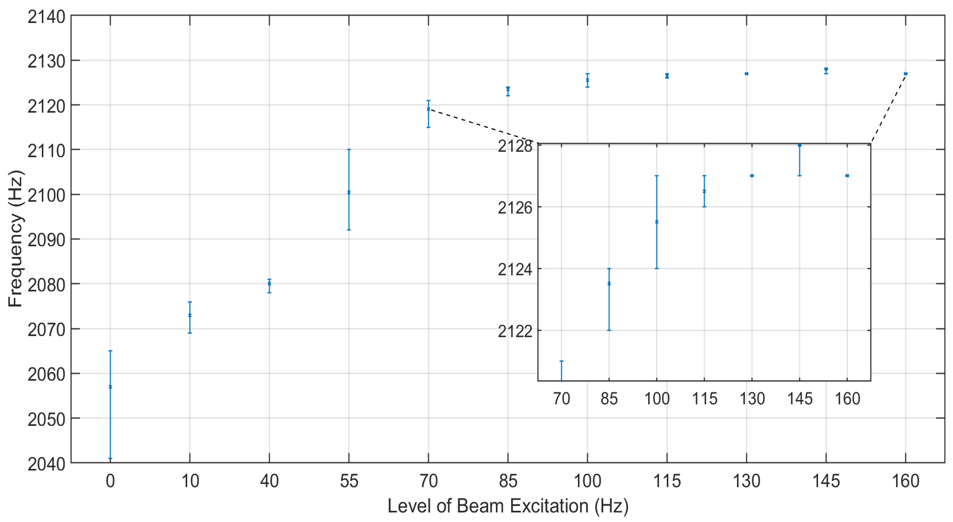
Figure 2, the Fourier plot of one representative signal from each test series shows that the bands of the dominant frequencies are consistently situated (in a decreasing order of magnitude) around 316 KHz, 1400 Hz, 1800 Hz and 2100 Hz. For each of these four frequency bands, the values of the dominant peaks are collected for each test series (six values per series), and the respective groups are plotted (in the form of error bars) in
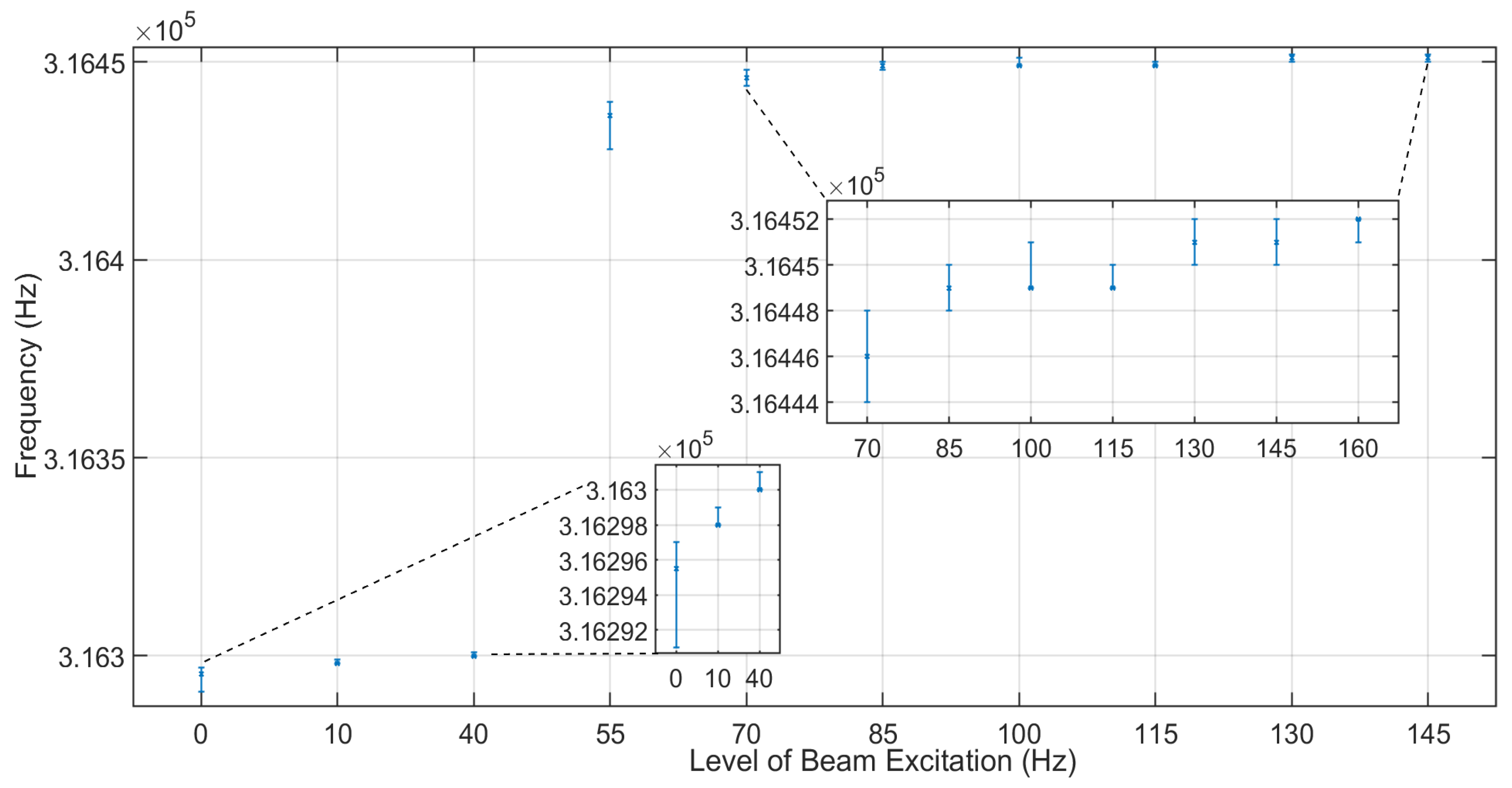
Figure 3,
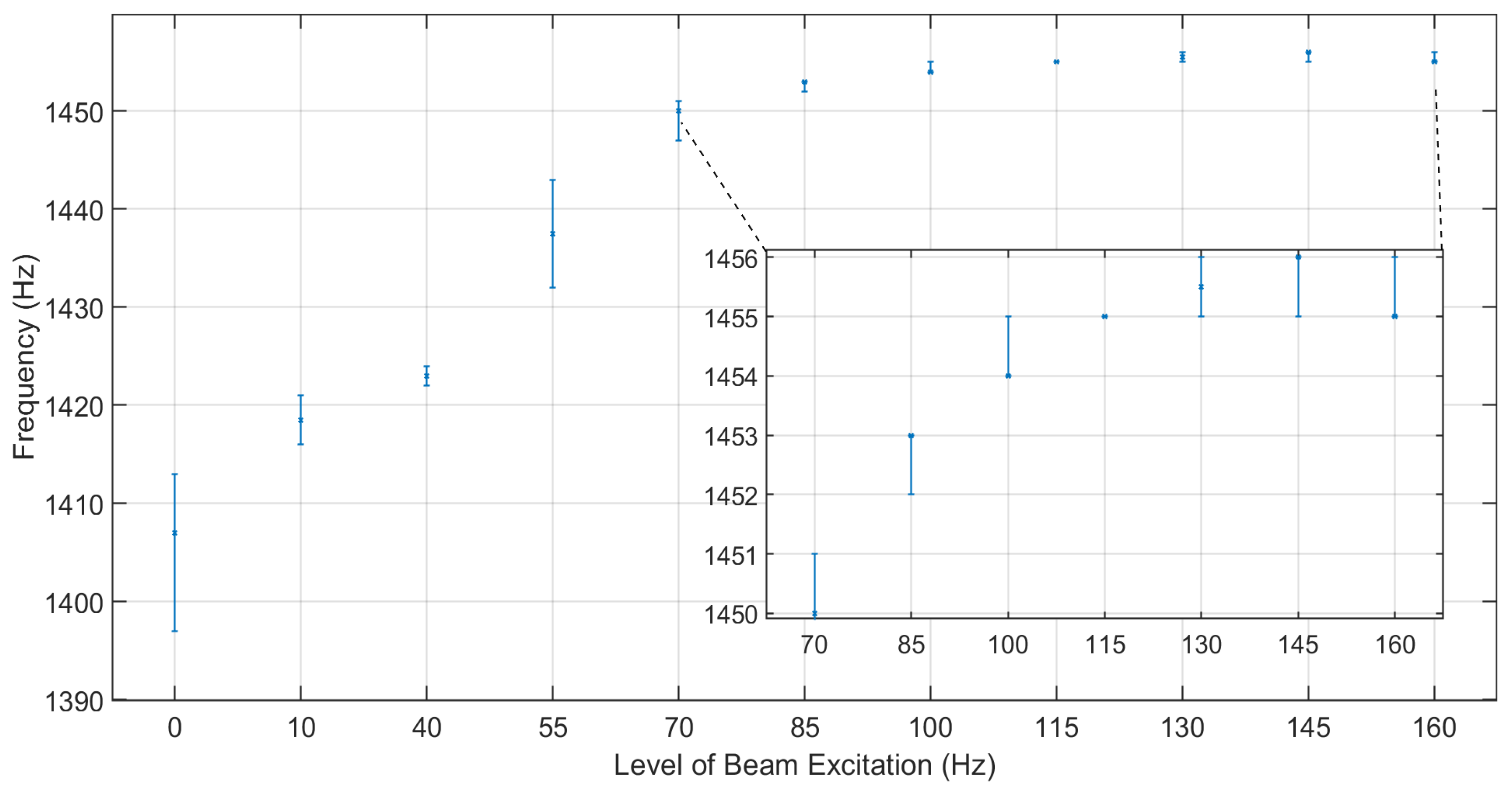
Figure 4,
Figure 5 and
Figure 6.
An initial remark is related to the groups resulting from the excitations at 10 Hz and 40 Hz, whose upper and lower values, respectively, are very close in all four frequency bands. This is indicative of the fact that an intermediate excitation level at 25 Hz was, indeed, not necessary since its group exhibited considerable overlapping neighboring groups. Then, it is easily noted that all groups up to 100 Hz feature an increasing trend with no apparent overlapping in frequency bands around 1400, 1800 and 2100 Hz. This, in turn, means that by focusing on the band around 1400 Hz and examining the frequency groups shown in
Figure 4,
Figure 5 and
Figure 6, a one-to-one mapping may be established between the beam excitation levels and the respective frequency peak groups. Hence, if a (voltage) signal’s frequency peak around, for instance, 1400 Hz is available, then one may deduce the excitation level of the beam simply using the previously mentioned mapping, provided that this level does not exceed 100 Hz.
This mapping becomes less consistent for excitation levels above 100 Hz, with
Figure 4 suggesting that the levels of 100 Hz are distinguishable from those of 115 Hz in the 1400 Hz band, or that the levels of 115 Hz are distinguishable from those of 130 Hz in the 316 KHz band (
Figure 3). In any case, a measure of the probability that two or more frequency groups are mutually distinguishable in each frequency band is required. For this purpose, the Kruskal–Wallis test is used between all possible pairs of groups to solve the hypothesis testing problem (1). The results, in terms of
p-values, are given in
Table 3,
Table 4,
Table 5 and
Table 6 for the frequency bands at 316 KHz, 1400 Hz, 1800 Hz and 2100 Hz, respectively.
In these tables, the intersecting cell of the
i-th line and the
j-th column presents the
p-value obtained using the Kruskal–Wallis test for the groups indicated in the respective line and column. Standard (non-shaded) cells correspond to cases where
H0 (groups with a similar distribution of data) is rejected in favor of
H1 (groups with a different distribution of data) at a risk level equal to α = 0.05, as explained in
Section 2.1. In such cases, the two groups considered are mutually distinguishable at the indicated risk level, meaning that the previously mentioned mapping is valid, again, at the indicated risk level. On the other hand, the shaded cells correspond to cases where
H0 (groups with a similar distribution of data) is accepted for the pair of groups under consideration, at a risk level equal to α = 0.05. Then, the two considered excitation frequencies would result in significantly overlapping groups of frequency peaks in the band of interest, meaning that no exclusive one-to-one mapping is possible. An examination of
Table 3,
Table 4,
Table 5 and
Table 6 basically validates the conclusions drawn by visual inspection of (the corresponding)
Figure 3,
Figure 4,
Figure 5 and
Figure 6. The frequency band around 1400 Hz provides statistically non-overlapping groups at a risk level of 0.05 (
Table 4) for beam excitation frequencies up to 115 Hz. Then, the excitation levels of 115 Hz and 130 Hz create overlapping groups (at a risk level of 0.05), since the p-value computed with the Kruskal–Wallis test is 0.055 (see the intersection between the ninth line and the tenth column), or just larger than 0.05, which leads to accepting the null hypothesis. At the same time,
p-values just larger than the risk level indicate a statistical tendency of being close to rejecting H
0. In other words, even though the 1400 Hz band does not actually allow for distinguishing between the excitation levels of 115 and 130 Hz, it would be relevant to look at other frequency bands for the null hypothesis being rejected when comparing the groups associated with the levels of 115 and 130 Hz. The band at 316 KHz offers this possibility since the
p-value (related to comparing groups created by the excitation levels of 115 Hz and 130 Hz—
Table 3) computed with the Kruskal–Wallis test is 0.0077 (see the intersection between the ninth line and the tenth column). However, in the band around 316 KHz, all groups created by the excitation levels above 130 Hz are statistically similar, as indicated by a
p-value of the Kruskal–Wallis test statistic equal to 0.2738 > 0.05 when comparing all three groups corresponding to the excitation levels of 130, 145 and 160 Hz. Then, distinguishing between the excitation levels of 115 and 130 Hz in the 316 KHz band may only be achieved in conjunction with p-values from the band around 2100 Hz in
Table 6. The latter indicates that the group resulting from the beam excited at 130 Hz cannot be mistaken for that associated with the excitation of 145 Hz at the considered risk level of 0.05. Thus, frequency peak groups resulting from excitation levels up to 145 Hz may be distinguished in a one-to-one comparison using the proposed setup and methodology.
Figure 3,
Figure 4,
Figure 5 and
Figure 6 and
Table 3,
Table 4,
Table 5 and
Table 6 suggest that a meaningful solution for distinguishing groups associated with excitation levels up to 145 Hz from a group associated with the excitation levels of 160 Hz is not available in all four bands considered.
A final remark regards these results with respect to the passive excitation principle used in this setup. Using mechanical excitation for the beam (and, hence, the magnetoelastic ribbon) without, for instance, some form of DC bias from a second coil [
20,
23] mainly allows for inducing sensing capabilities in standard conventional beams in a cost-effective manner. On the other hand, the recorded signal is quite noisy, meaning that more (and surely non-trivial) algorithmic effort has to be invested in rejecting noise effects and obtaining results on higher-order modes of vibrations and/or larger beam deflections.
3.2. Results of the Statistical Evaluation of Fault Diagnosis Characteristics
The testing procedure involved six experiments per fault case (or test scenario as referred to) in
Table 1. The 48 voltage signals resulting from the testing were also used in [
24] along with the three-step procedure outlined in
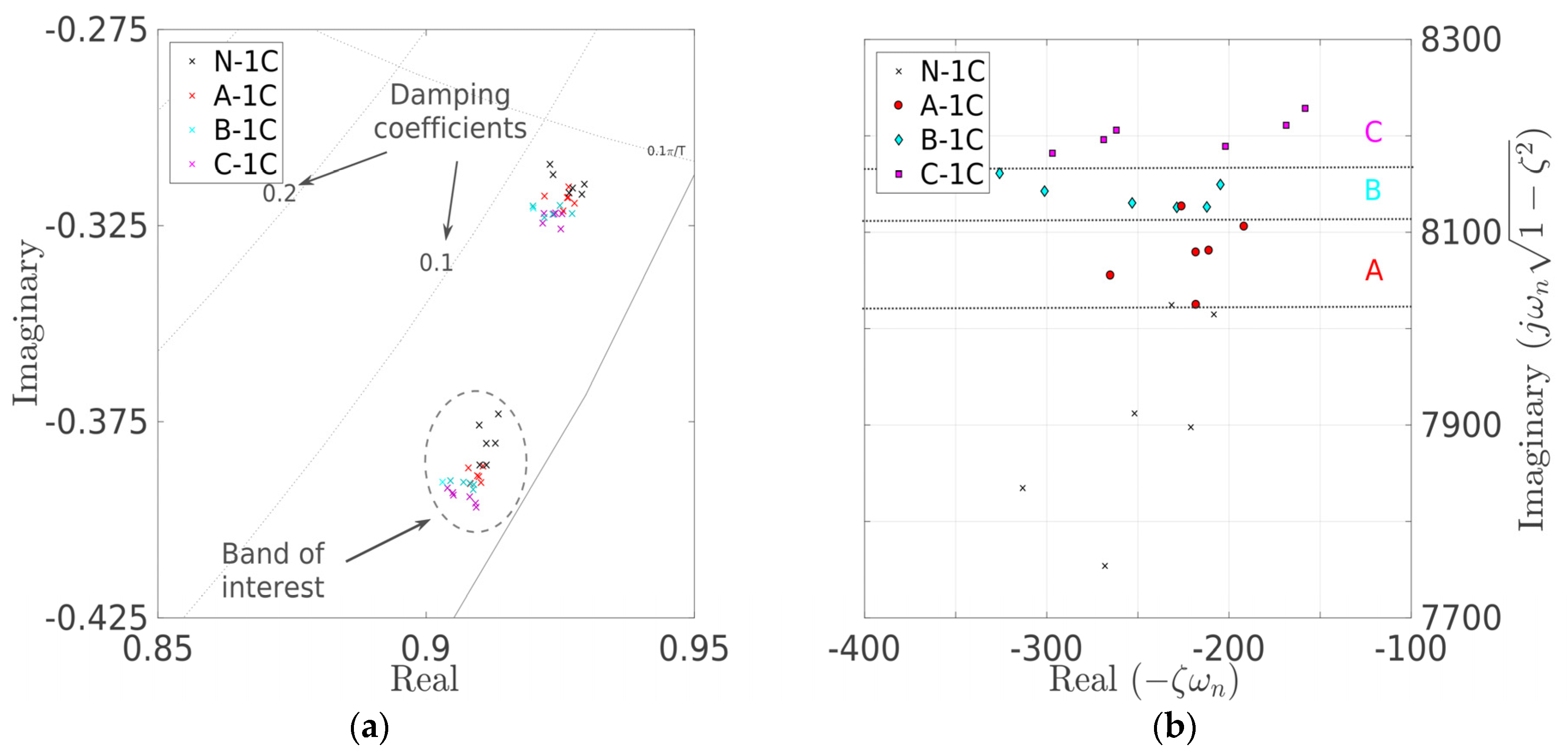
Section 2.2, to deliver initially the discrete-time AR poles inside the bands of the dominant frequencies (around 1350–1400 Hz in this case) and then their corresponding continuous-time counterparts. This yielded the pole areas in
Figure 7a,b at the z-plane and the s-plane, respectively, for the –1C fault cases.
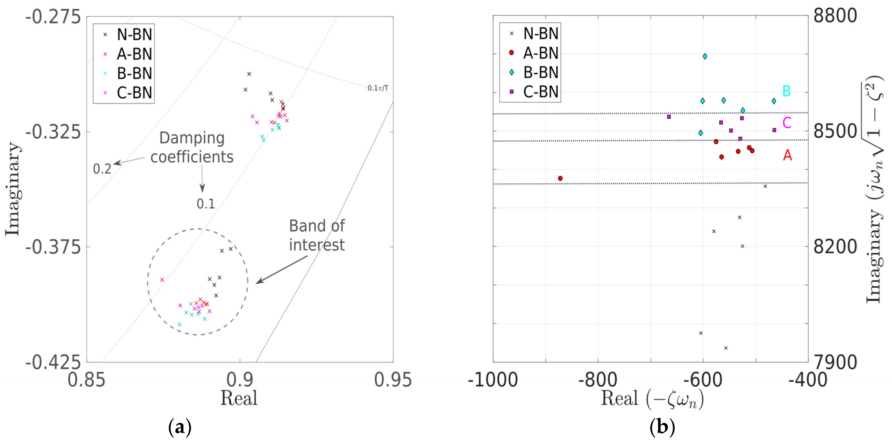
Figure 8a,b presents the pole areas at the z-plane and the s-plane, respectively, for the –BN fault cases. From these figures, it seems quite hard to visually distinguish groups of poles corresponding to specific pole scenarios in discrete time (z-plane), whereas it is relatively easier to distinguish these groups in continuous time (s-plane). But even when the s-plane is considered, poles corresponding to the N-1C beam configuration may be found in the area involving poles corresponding to the A-1C-affected beam (
Figure 7b). In other words, the corresponding pole groups seem to effectively (although slightly) overlap. The same is obvious for the A-1C and B-1C poles, as well as the poles from the B-BN- and C-BN-affected beams (
Figure 8b). Hence, although, in principle, –1C or –BN faults of all magnitudes and positions on the beam may be distinguished from each other, a statistical assessment of (overlapping) pole groups would be desirable. This assessment would quantify the inherent uncertainty when fault diagnosis (detection, isolation and magnitude estimation) is carried out by examining regions where these pole groups are located on the s-plane.
The statistical assessment of whether the regions of continuous-time pole groups corresponding to fault cases (test scenarios) are distinguishable between them may be carried out by formulating the statistical hypothesis problem (2), as described in
Section 2.2. The Kruskal–Wallis test is again used for pairs of pole groups and addresses the hypothesis testing problem at a risk level α equal to 0.05. Only imaginary parts of the poles for each group are considered as pole coordinates since pole regions are delimited with respect to their imaginary part in
Figure 7b and
Figure 8b. The detection of fault occurrence for fault types –1C and –BN is examined by forming
Table 7 and
Table 8, respectively. The intersecting cell of the
i-th line and the
j-th column presents the
p-value obtained using the Kruskal–Wallis test for the fault cases indicated in the respective line and column. The shaded cells correspond to significantly overlapping groups of poles.
In
Table 7,
H0 is systematically rejected for any comparison of N-1C against the A, B or C-1C fault cases, at α = 0.05, since in all such cases, the
p-value is lower than α. In other words, the (imaginary parts of the) poles from the N-1C configuration do not follow a similar distribution as those from the A, B or C-1C configurations at α = 0.05, and faults may be systematically detected. Again, in
Table 7,
H0 is systematically rejected for any comparison of N-1C against the A, B or C-1C fault cases at α = 0.05. Hence, all –1C fault cases have different impacts on the pole (imaginary) locations, meaning that all –1C faults may be identified. Note, however, that the
p-value for comparing the A-1C and B-1C configurations is notably higher (see the intersection between the third line and the fourth column), although smaller than α = 0.05. This is related to the overlap between the two groups, as seen in
Figure 7b, which was commented upon earlier on. The same conclusions in terms of detection and identification may be drawn for the –BN configurations with a careful examination of
Table 8. Again, comparing the B-BN and C-BN configurations results in a higher-than-usual
p-value (although again smaller than α = 0.05), which is related to the slight overlap of groups designating the B-BN and C-BN fault cases in
Figure 8b. Lastly,
Table 9 allows for addressing the issue of distinguishing between the fault configurations –1C (small fault magnitude) and –BN (large fault magnitude), as defined in
Table 1. Again, the shaded cells correspond to significantly overlapping groups of poles. In general, the
p-values are always smaller than α = 0.05, meaning that
H0 is systematically rejected at the risk level α = 0.05 for all comparisons between the –1C and –BN configurations. Then, no –BN fault may be mistaken for a –1C fault at the designated risk level. Obviously, these results are valid for cases of a single fault (load) occurrence at a time.
Note that formulating the statistical hypothesis problem (2), as described in
Section 2.2, proved again to be highly beneficial for discrete-time pole groups in the z-plane. As noted before, in [
24], it was hard to delimit specific z-plane pole areas associated with the fault cases of
Table 1 using a simple visual inspection. In the current study, the Kruskal–Wallis test is again used for pairs of discrete-time pole groups (see
Figure 7a and
Figure 8a) in order to address the hypothesis testing problem at a risk level α equal to 0.05. For each such pole, its angle of rotation with respect to the origin is considered, and specifically, the ratio of its imaginary over its real part (effectively corresponding to the tangent of that angle). The detection of fault occurrence for the fault types –1C and –BN is examined by forming
Table 10 and
Table 11, respectively. As in the continuous-time case, the intersecting cell of the
i-th line and the
j-th column presents the
p-value obtained using the Kruskal–Wallis test for the fault cases indicated in the respective line and column. The shaded cells correspond to significantly overlapping groups of poles. The results are equivalent to those obtained for the s-plane pole groups, with
H0 systematically rejected for any comparison of N-1C against the A, B or C-1C fault cases, at α = 0.05, as shown in
Table 10.
The same comments hold for results presented in
Table 11, with
H0 systematically rejected for any comparison of N-BN against the A, B or C-BN fault cases, at α = 0.05. Again, one may distinguish between the s –1C (small fault) and –BN (large fault) configurations in
Table 1 using rotation angles of the discrete-time poles in the z-plane to form
Table 12. As in the continuous-time case, the
p-values are always smaller than α = 0.05, meaning that
H0 is systematically rejected at the risk level α = 0.05 for all comparisons between the –1C and –BN configurations. Then, no –BN fault may be mistaken for a –1C fault at the designated risk level, even using discrete-time AR poles. As in the continuous-time case, these results are valid for cases of a single fault (load) occurrence at a time.
A remark may at this point be made on having relatively few data values in each group when the comparisons between two or more groups are carried out using the Kruskal–Wallis test. As noted in
Section 2, the Kruskal–Wallis test may be used with groups of five or more data values each [
25,
26,
27], with relevant examples in [
25], ch. 8, and in [
26], ch. 25. It is clear that in the current study, this condition is fulfilled. Nonetheless, it would be advisable to use more data values per group since this would render the Kruskal–Wallis test more powerful. Currently, the test is more conservative rather than powerful in the sense that it is more reluctant to reject the null hypothesis
H0 at the designated risk level. This, in turn, means that the results presented both for sensing and for fault diagnosis purposes are rather conservative. In terms of evaluating sensing characteristics, for instance, if more data per group were available, then comparisons between certain groups at the band around 1400 Hz (which indicated overlapping groups due to the
p-values being marginally higher than α = 0.05) could yield results toward rejecting
H0, thus enabling a distinction between the groups considered.
A final remark is related to these sensing and fault diagnosis results being obtained for a long, thin and flexible beam. The same basic setup with a model-based algorithmic framework was applied to shorter, thicker and quite more rigid polymer beams in the previous works [
17] and (in part) [
18], with similarly successful fault diagnosis results. Nonetheless, sensing properties were not comprehensively evaluated in these studies since they both aimed at obtaining fault diagnosis results. Moreover, no experiments with steel structures have been carried out yet. Specifically, for such cases, the applicability of the proposed setup and algorithmic analysis in terms of sensing and fault diagnosis has yet to be tested, even though the currently obtained results are promising.


