Article

Energy-Preserving/Group-Preserving Schemes for Depicting Nonlinear Vibrations of Multi-Coupled Duffing Oscillators

1
Center of Excellence for Ocean Engineering, National Taiwan Ocean University, Keelung 202301, Taiwan
2
Department of Mechanical Engineering, National United University, Miaoli 360302, Taiwan
*
Author to whom correspondence should be addressed.
Vibration 2024, 7(1), 98-128; https://doi.org/10.3390/vibration7010006
Submission received: 21 November 2023 / Revised: 18 December 2023 / Accepted: 12 January 2024 / Published: 18 January 2024
(This article belongs to the Special Issue Feature Papers in Vibration)

Abstract

:
In the paper, we first develop a novel automatically energy-preserving scheme (AEPS) for the undamped and unforced single and multi-coupled Duffing equations by recasting them to the Lie-type systems of ordinary differential equations. The AEPS can automatically preserve the energy to be a constant value in a long-term free vibration behavior. The analytical solution of a special Duffing–van der Pol equation is compared with that computed by the novel group-preserving scheme (GPS) which has fourth-order accuracy. The main novelty is that we constructed the quadratic forms of the energy equations, the Lie-algebras and Lie-groups for the multi-coupled Duffing oscillator system. Then, we extend the GPS to the damped and forced Duffing equations. The corresponding algorithms are developed, which are effective to depict the long term nonlinear vibration behaviors of the multi-coupled Duffing oscillators with an accuracy of  O ( h 4 )  for a small time stepsize h.

1. Introduction

In our real world, the nonlinear vibrational phenomena are ubiquitous, mainly modeled by nonlinear ordinary differential equations. Nonlinear vibrations and their periodic motions are important topics [1]; the study of related issues from nonlinear vibrations is greatly important for many practical applications, which are considered not only in mechanics and physics but also in other disciplines of science. In this paper, a quite powerful numerical integration method, namely an automatically energy-preserving scheme (AEPS), is developed to solve the following Duffing equation:
x ¨ ( t ) + γ x ˙ ( t ) + α x ( t ) + β x 3 ( t ) = f ( t ) ,
as well as multi-coupled Duffing equations.
Almost a century ago, the Duffing equation was derived [2]. Nowadays, it describes vibrational motion with more complex phenomena than the harmonic motion, showing rich behavior of period-doubling route to chaos and displaying vibration jumps in the changing frequency for the forced oscillator with nonlinear restoring force. A lot of applications of Duffing equations in science and engineering have appeared [3,4,5,6,7,8]. Computational methods gave been developed for solving the transient and steady oscillatory problems of nonlinear Duffing equations [9,10,11,12,13,14,15,16,17,18,19,20,21,22,23].
Analytical methods have been reviewed by Cveti c ´ anin [2] for the unforced and undamped Duffing equation, presented in the form of some elliptic functions. In general, for nonlinear Duffing equations, there exists no analytical solution, and some semi-analytical methods such as as the power series and harmonic balance methods, have to be invoked [24,25,26]. In continuous works, Liu et al. [27] developed the scaled power series techniques for solving the Duffing equation.
Since the works of Liu [28], the group-preserving scheme (GPS) was applied in many places of the scientific computations. Akgül et al. [29] developed a group-preserving scheme method for the Poisson–Boltzmann equation for semiconductor devices. Hashemi et al. [30] applied the group-preserving scheme method to the one-dimensional hyperbolic telegraph equation by line discretization. In [31], a powerful group-preserving scheme was presented to solve the Klein–Gordon equation, where graphs of the exact solution, numerical solution, absolute error and the contour plot of error were provided successfully. The GPS is a robust method used to solve different problems such as fractional Poisson equation [32], the fractional diffusion equation [33], the Cauchy problem [34], the sine-Gordon equation [35], and the Burgers equation [36]. Recently, Xu and Wu [37] developed the MGPS: a midpoint-series group-preserving scheme for solving a quite general nonlinear dynamics system. Partohaghighi et al. [38] applied the group-preserving scheme method to solve fractional differential equations.
The most famous Lie-group is the three-dimensional rotation group denoted as  G , which is a single parameter of time t to describe the motion  x ( t )  of a rigid body in  R 3 . When initial state  x ( 0 )  has a certain length  x ( 0 ) > 0 , then the Lie-group action by  G ( t ) S O ( 3 ) :
x ( t ) = G ( t ) x ( 0 ) ,
keeps the length invariant,
x ( t )   =   x ( 0 ) ,
due to
G T ( t ) G ( t ) = I 3 .
The corresponding Lie-algebra of  S O ( 3 )  is  A s o ( 3 ) , satisfying
A T g + g A = 0 ,
where
g = 1 0 0 0 1 0 0 0 1
is a metric tensor of  R 3 . In  g , we have three positive identities on the diagonal, which is then said to have a signature  ( 3 , 0 ) . General space  R p , q  with p positive identity and q negative identity is a pseudo-Euclidean space, whose invariant Lie-group  G = exp ( t A ) S O ( p , q )  satisfies
G T ( t ) g G ( t ) = g ,
where  A s o ( p , q )  and  g  has p positive identity and q negative identity on the diagonal. The pseudo-Euclidean length of  x ( t ) R n , n = p + q  is invariant under  G ( t ) S O ( p , q ) :
x T ( t ) g x ( t ) = x T ( 0 ) g x ( 0 ) .
Inserting Equation (2) for  x ( t )  into the left-hand side, we have
x T ( t ) g x ( t ) = x T ( 0 ) G T g G x ( 0 ) ,
which, by Equation (7), proves Equation (8).
Because  G  in Equation (2) can preserve the quadratic form invariant, the developed numerical integration method called a group-preserving scheme (GPS) is better than the traditional Runge–Kutta integration method. However, for the nonlinear Duffing coupled oscillators system, this task is difficult, which is not at all trivial work. Our principal goal is developing the  S O ( p , q )  Lie-group integrator for such a complex system to preserve energy automatically.
Among the attempts to address the issue of energy preservation, the projection and symmetric projection techniques are coupled with symplectic schemes to enforce the numerical solution to lie on a proper manifold of energy conservation. Simo et al. [39] introduced energy-preserving schemes for unconstrained rigid bodies, nonlinear dynamics of beams and shells and nonlinear elastodynamics, devised a one-parameter family of symplectic integrators by determining that the time stepsize takes place on the level of constant angular momentum, and showed that the parameter may be suitably tuned in a way to enforce the conservation of energy. Earlier, Liu [40] proposed a method to keep the constraints of a nonlinear dynamical system by adjusting the integrating factors. In addition, there are several energy-preserving integrators [41,42,43,44,45,46]. In general, these schemes used to enforce energy conservation are quite time consuming, and are not performed automatically.
For its vital role of an energy-conserving technique in different systems, many applications and energy-conserving methods have been presented, e.g., a 3D stochastic nonlinear Schrödinger equation with multiplicative noise [47], a nonlinear Schrödinger equation [48], nonlinear wave equations with dynamic boundary conditions [49], nonlinear space fractional Schrödinger equations with a wave operator [50], the pitch-angle scattering in magnetized plasmas [51], the nonlinear Dirac equation [52], the linear wave equation [53], the Rosenau-type equation [54], nonlinear fourth-order wave equations [55], the multi-dimensional Hermite-DG discretization of Vlasov–Maxwell equations [56], the Vlasov–Ampère system [57], the Vlasov–Ampère system with an exact curl-free constraint [58], relativistic Vlasov–Maxwell equations of laser–plasma interaction [59], the linear wave equation with forcing terms [60], Hamiltonian systems (including the high amplitude vibration of strings and plates) [61], the multi-dimensional Vlasov–Maxwell system [62], generalized nonlinear fractional Schrödinger wave equations [63].
The novelties involved in the paper are as follows:
  • For the single, two-coupled and three-coupled undamped and unforced Duffing equations, novel methods to automatically preserve energy were developed.
  • Detailed formulations of energy invariants, variable transformations, Lie algebras and Lie groups used in long-term computations of nonlinear free vibrations were derived.
  • For the damped and unforced Duffing equations, group-preserving schemes were developed at the first time.
  • Highly accurate solutions of responses were obtained.
The paper is organized as follows. In Section 2, we introduce a novel variable transformation and the AEPS for hardening and softening cases of the Duffing equation without considering the damping term and external force; the resulting Lie groups are, respectively,  S O ( 2 )  and  S O ( 1 , 1 ) . Then, in Section 3, we extend the Lie-group scheme to a group-preserving scheme (GPS) for solving the forced Duffing equation equipped with a damping term. In Section 4, we develop the GPS for the Duffing–van der Pol equation, where the Poincar e ´  section is used to display the chaotic behavior of Duffing–van der Pol equation. In Section 5.1, we develop the Hamiltonian form for coupled Duffing equations. Lie-type forms and AEPS for two coupled Duffing equations without considering damping effect and external force are developed in Section 5.2 and Section 5.3; the resulting Lie-groups, depending on the parameters of nonlinear springs, are divided into three types:  S O ( 4 ) S O ( 3 , 1 ) , and  S O ( 2 , 2 ) . The group-preserving schemes for the damped and forced two coupled Duffing equations are developed in Section 5.4. Section 6 solves the three coupled Duffing equations considering damping and external force; the resulting Lie-groups, depending on the parameters of nonlinear springs, are divided into four types:  S O ( 6 ) S O ( 5 , 1 ) S O ( 4 , 2 )  and  S O ( 3 , 3 ) . Finally, we conclude the paper in Section 7.

2. An Automatically Energy-Preserving Scheme

To demonstrate energy-preserving behavior, we consider an unforced Duffing equation:
x ¨ ( t ) + α x ( t ) + β x 3 ( t ) = 0 ,
which does not include a damping term to be an undamped Duffing oscillator. Taking the product of the above equation with  x ˙ ( t )  and integrating it leads to
d d t 1 2 x ˙ 2 ( t ) + α 2 x 2 ( t ) + β 4 x 4 ( t ) = 0 ,
1 2 x ˙ 2 ( t ) + α 2 x 2 ( t ) + β 4 x 4 ( t ) = C ,
where C is constant energy determined by initial values with  C = x ˙ 2 ( 0 ) / 2 + α x 2 ( 0 ) / 2 + β x 4 ( 0 ) / 4 . Equation (12) indicates that the energy combined kinetic energy and potential energy is a constant value, which inspires us to develop an AEPS.
The energy-preserving condition in space  ( x , x ˙ )  renders a framework from the differentiable manifold and its Lie-group transformation, which played a decisive role in devising superior numerical methods [28,64,65,66]. As shown by Liu [67], the Lie-group scheme can find an approximation of
Y ˙ = A ( Y , t ) Y , Y ( 0 ) = Y 0 ,
where  A  is a matrix Lie-algebra, and  Y  is the corresponding matrix Lie-group.
The AEPS can automatically preserve energy  x ˙ 2 / 2 + α x 2 / 2 + β x 4 / 4  in Equation (12) for both the hardening case  β > 0  and th softening case  β < 0 , in the undamped and unforced Duffing equation, i.e.,  γ = 0  and  f = 0 . However, developing a numerical integrating method which can automatically preserve energy is not a trivial task; it needs some mathematical analysis.
Equation (8) reveals that the invariant form must be quadratic, which is permitted by Lie-group action in Equation (7). However, energy Equation (12) is not of quadratic form owing to the appearance of  x 4 ( t ) ; hence, the Lie-group cannot be applied directly. Below, we recast Equation (12) to a quadratic form by the transformation to new variables, such that benefit can be gained by Lie-group Equation (7), which can bring out a novel method for the preservation of energy automatically as shown in Equation (8). Before the construction of the Lie-group  G , we must derive the Lie-algebra  A  in the Lie-type system as shown in Equation (13).

2.1. Lie-Group  S O ( 2 )  for  β > 0

First, we consider the case with  β > 0 . Then, Equation (12) can be written as
x ˙ 2 ( t ) + β 2 x 2 ( t ) + α β 2 = 2 C + α 2 2 β ,
where the right-hand side is a constant value determined by given initial values  x ( 0 )  and  x ˙ ( 0 ) , and parameters  α  and  β .
We let
y ( t ) : = β 2 x 2 ( t ) + α β
be a new variable to replace x; hence, we have
x ˙ 2 ( t ) + y 2 ( t ) = 2 C + α 2 2 β ,
which shows that  ( y , x ˙ )  is located on a circle with a radius of  2 C + α 2 / ( 2 β ) .
Using Equations (10) and (15), we can derive
d d t y x ˙ = 0 2 β x 2 β x 0 y x ˙ ,
which belongs to Equation (13). Because the coefficient matrix is skew-symmetric, the resulting Lie-group is  S O ( 2 ) , of which constant matrix
A ¯ k : = 0 2 β x ¯ k 2 β x ¯ k 0
is available for a small time increment, where  x ¯ k = ( 1 θ ) x k + θ x k + 1  and  x k  and  z k = x ˙ k  are the numerical values of x and  x ˙  given at the previous time step. The corresponding Lie-group  G k S O ( 2 )  is obtained by exponential mapping:
G k = exp ( h A ¯ k ) = cos ( 2 β x ¯ k h ) sin ( 2 β x ¯ k h ) sin ( 2 β x ¯ k h ) cos ( 2 β x ¯ k h ) .
The resulting AEPS reads as follows:
(i)
We give  0 θ 1 , h ε  and  ( x 0 , z 0 ) = ( x 0 , x ˙ 0 ) .
(ii)
For  k = 0 , 1 , ,
x k + 1 = x k + h z k , z k + 1 = z k h ( α x k + β x k 3 ) , y k + 1 = β 2 x k + 1 2 + α β .
(iii)
We compute
x ¯ k = ( 1 θ ) x k + θ x k + 1 , y ^ k + 1 z ^ k + 1 = cos ( 2 β x ¯ k h ) sin ( 2 β x ¯ k h ) sin ( 2 β x ¯ k h ) cos ( 2 β x ¯ k h ) y k z k , x k + 1 = ± 2 β y ^ k + 1 α β 1 / 2 .
If the convergence is satisfied,
( y ^ k + 1 y k + 1 ) 2 + ( z ^ k + 1 z k + 1 ) 2 < ε ,
then we proceed to (ii) for the next time step; otherwise, we let  y k + 1 = y ^ k + 1  and  z k + 1 = z ^ k + 1 , and proceed to (iii).
We fix  θ = 1 / 2  for all computations given below. The iteration part in (iii) is used to enhance the accuracy of Lie-algebra  A ¯ k  in Equation (18), and hence the accuracy of the numerical solution to the designed criterion  ε  can be achieved. Part (iii) is not for the preservation of energy, because the Lie-group integrator AEPS is already automatically preserving the energy without any iteration.

2.2. Lie-Group  S O ( 1 , 1 )  for  β < 0

Next, we consider the case with  β < 0 . Upon letting
y ( t ) : = β 2 x 2 ( t ) + α β
be a new variable, it follows from Equation (14) that
x ˙ 2 ( t ) y 2 ( t ) = 2 C + α 2 2 β ,
which reveals that point  ( y , x ˙ )  is located on a hyperbola in the plane.
Using Equations (10) and (23),
d d t y x ˙ = 0 2 β x 2 β x 0 y x ˙
is just the form of Equation (13).
Because the coefficient matrix is symmetric, the resulting Lie-group is  G k S O ( 1 , 1 ) , whose implicit scheme based on  S O ( 1 , 1 )  for the integration of Equation (10) with  β < 0  is
A ¯ k : = 0 2 β x ¯ k 2 β x ¯ k 0 ,
G k = exp ( h A ¯ k ) = cosh ( 2 β x ¯ k h ) sinh ( 2 β x ¯ k h ) sinh ( 2 β x ¯ k h ) cosh ( 2 β x ¯ k h ) .
The resulting AEPS: (i) we offer h 0 θ 1 ε  and  ( x 0 , z 0 ) = ( x 0 , x ˙ 0 ) ; (ii) for  k = 0 , 1 , ,
x k + 1 = x k + h z k , z k + 1 = z k h ( α x k + β x k 3 ) , y k + 1 = β 2 x k + 1 2 + α β ;
(iii) the new  ( y k + 1 , z k + 1 )  is iteratively solved by
x ¯ k = ( 1 θ ) x k + θ x k + 1 , y ^ k + 1 z ^ k + 1 = cosh ( 2 β x ¯ k h ) sinh ( 2 β x ¯ k h ) sinh ( 2 β x ¯ k h ) cosh ( 2 β x ¯ k h ) y k z k , x k + 1 = ± 2 β y ^ k + 1 α β 1 / 2 .
If convergence is satisfied by
( y ^ k + 1 y k + 1 ) 2 + ( z ^ k + 1 z k + 1 ) 2 < ε ,
then we proceed to (ii); otherwise, we let  y k + 1 = y ^ k + 1  and  z k + 1 = z ^ k + 1 , and procewed to (iii) for computing Equation (29).

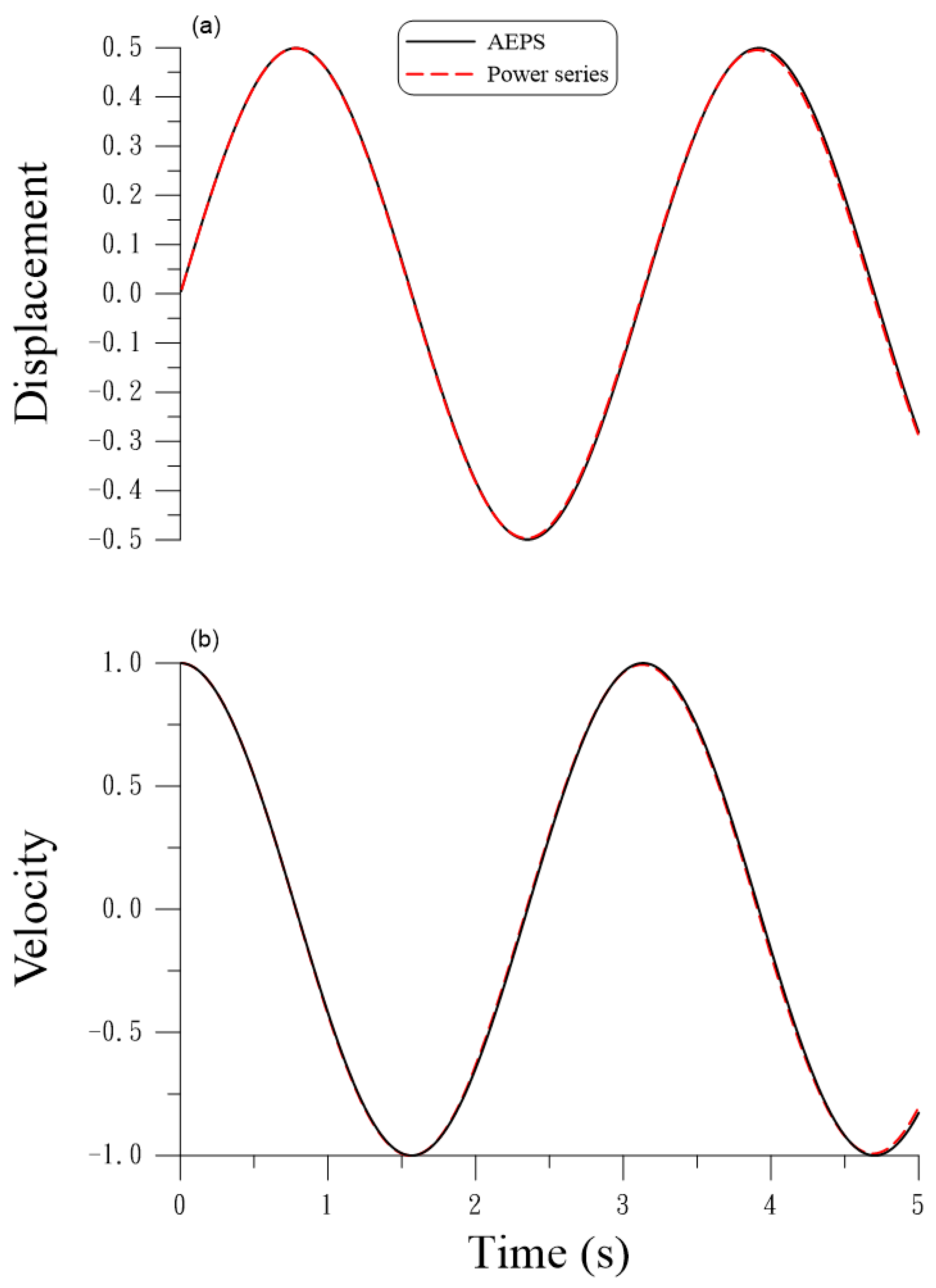
2.3. Testing the Efficiency of AEPS

For testing the performance of AEPS, Equation (10) under the same initial conditions  x ( 0 ) = 0  and  x ˙ ( 0 ) = 1  is considered, with the same parameter value  α = 4  but different parameter values of  β = 0.1  and  β = 0.01 .
We solve the first problem with  β = 0.1  using the AEPS with  h = 0.001  and  ε = 10 10 , and compare the responses with those obtained by the power series method (PSM) [25]. As shown in Figure 1 in the time range of  t [ 0 , 5 ] , these two solutions are almost coincident. The exact value of  C = 0.5  is compared with that computed by the AEPS and the PSM, of which the errors of energy defined by  | z k 2 / 2 + α x k 2 / 2 + β x k 4 / 4 C |  are compared in Figure 2a. It can be seen that the capability of the AEPS is much better than that of the PSM in the preservation of energy. The errors of energy obtained by the AEPS are in the range from  10 12  to  10 14 ; however, the errors of energy obtained by the PSM are fast tending to  10 2 .
Even under a stringent convergence criterion with  ε = 10 10 , the AEPS converges very fast with 2 or 3 iterations at each time step.
We compare the responses for the second problem with  β = 0.01  obtained by the AEPS with those obtained by the power series method (PSM) [25]. As shown in Figure 3, in the time range of  t [ 0 , 5 ] , these two solutions are almost coincident. The exact value of  C = 0.5  is compared with that computed by the AEPS and the PSM with  z k 2 / 2 + α x k 2 / 2 + β x k 4 / 4  being the numerical values of the energy, of which the errors of energy are compared in Figure 2b. The errors of energy obtained by the AEPS are in the range from  10 10  to  10 13 ; however, the errors of energy obtained by the PSM are fast tending to  10 3 . The accuracy of the AEPS is much better than that of the PSM in the preservation of energy.
Lie-groups  G k  as shown in Equation (19) for  β > 0  and Equation (27) for  β < 0  possess the following property:
det G k = 1 ,
which indicates that  G k  has a constant determinant equal to one. Therefore, iteration Part (iii) in each algorithm converges to a fixed point on the manifold specified by Equation (31). Part (iii) is crucial to determine the accurate value of  G k , such that the predicted values in (ii) are corrected to the accurate values on the energy-preserved manifold.

2.4. General Setting

Upon comparing two different formulations in Section 2.1 for the hard spring Duffing oscillator with  β > 0 , and in Section 2.2 for the soft spring Duffing oscillator with  β < 0 , we can summarize the key points as follows:
Hard spring : g = 1 0 0 1 , A s o ( 2 ) , G S O ( 2 ) ,
Soft spring : g = 1 0 0 1 , A s o ( 1 , 1 ) , G S O ( 1 , 1 ) .
The corresponding quadratic forms to signify the energy conservation are different, with Equation (16) for hard spring case  β > 0  and Equation (24) for soft spring case  β < 0 .
As for multi-coupled Duffing oscillators to be discussed below, the situation becomes more complex with many different cases needing to be considered for the metric tensors, Lie-algebras, Lie-groups and the quadratic forms of energy equations. Therefore, we outline a general setting of the numerical algorithm, namely the AEPS, given as follows.
When  x  represents the original variables,  y  expresses the transformed variables, whose Lie-type equation is
y ˙ ( t ) = A ( y ) y ( t ) .
In terms of matrix–vector notations, the algorithm can be written more clearly as follows:
(i)
We give  y 0 = y ( 0 ) θ ε , step size h t 0 = 0  and a final time  t f > 0 .
(ii)
For  k = 0 , 1 , t k + 1 = t k + h t f , we predict, by an Euler step,
y k + 1 = y k + h A k y k = y k + h A ( y k ) y k .
(iii)
We compute
y ¯ k = ( 1 θ ) y k + θ y k + 1 ,
G k = exp [ h A ( y ¯ k ) ] ,
y ^ k + 1 = G k y k .
If
y ^ k + 1 y k + 1 < ε ,
then we proceed to (ii) for the next time step; otherwise, we let  y k + 1 = y ^ k + 1 , and proceed to (iii).
The above numerical processes guarantee that new state variable  y k  at each time step preserves the quadratic invariant,
y k T g y k = y 0 T g y 0 ,
such that the energy is preserved. Because the restoring force of the Duffing equation is a cubic nonlinear function of the state variable, the transformation of the energy equation to a quadratic form is not a trivial task. Difficulty especially arises when the dimension of the Duffing equation system is increased. The work to construct the Lie-algebra, Lie-symmetry and the quadratic form of the energy-conserving equation becomes more difficult and challenged for the multi-coupled Duffing oscillator system. The major novelty of the constructions of these mathematical tools is not yet existent in the literature for the multi-coupled Duffing oscillator system. Below, we explore these interesting issues for single, two-coupled and three-coupled Duffing oscillator systems. When the quadratic invariant can be guaranteed by the proposed algorithm, the energy of the system can be conserved automatically. For this reason, the automatically constructed energy-preserving scheme (AEPS) has high performance of the computational ability to observe the long-term vibration behavior, unlike the traditional numerical methods, like as the Runge–Kutta method.
The existing methods mentioned in Section 1 need the projection technique such that they do not automatically preserve the energy. In the AEPS, the energy equation must be transformed to a quadratic form to a pseudo-sphere in space  R p , q , which is a limitation of the AEPS for needing to seek for a suitable transformation between original variables and new variables. Of course, to construct such type of transformation is itself a great challenge.

3. The GPS for Equation (1)

Now, we return to Equation (1) with  β > 0 , of which, using Equation (15), we can derive
d d t y x ˙ = 0 2 β x 2 β x γ y x ˙ + 0 f ( t ) .
Letting
A : = 0 2 β x 2 β x γ ,
we can observe that
A = S + W , S = 0 0 0 γ , W = 0 2 β x 2 β x 0 ,
where  S  and  W  are, respectively, the symmetric part and the skew-symmetric part of  A . According to Liu [68], the Lie-group generated is a dilation rotation group, denoted by  D S O ( 2 ) . The advantage of the group-preserving scheme (GPS) can be continued, if we can derive the corresponding Lie-group  G  by the exponential mapping, such that  G D S O ( 2 ) . This is performed below for the damped and forced Duffing oscillator system.
To apply the trapezoidal rule for the non-homogeneous term, the group-preserving scheme (GPS) is obtained as follows:
y k + 1 x ˙ k + 1 = G k y k x ˙ k + 0 h 2 f ( t k + 1 ) + h 2 G k 0 f ( t k ) ,
where
G k = exp ( h A ¯ k ) ,
A ¯ k : = 0 2 β x ¯ k 2 β x ¯ k γ .
We let
a : = 2 β x ¯ k , b : = a 2 γ 2 4 ,
and through some derivations, we can obtain
G k = e γ h / 2 cos ( b h ) e γ h / 2 sin ( b h ) e γ h / 2 2 a [ γ cos ( b h ) + 2 b sin ( b h ) ] e γ h / 2 2 a [ 2 b cos ( b h ) γ sin ( b h ) ] 1 0 γ 2 b a b , i f a 2 γ 2 4 > 0 ,
G k = e γ h / 2 cosh ( b h ) e γ h / 2 sinh ( b h ) e γ h / 2 2 a [ 2 b sinh ( b h ) γ cosh ( b h ) ] e γ h / 2 2 a [ 2 b cosh ( b h ) γ sinh ( b h ) ] 1 0 γ 2 b a b , i f a 2 γ 2 4 < 0 .
In Figure 4, we display a typical response of the Duffing equation with  γ = 0  and under a periodic force  f = f 0 sin ( ω t ) . We compute the response for parameters  α = 1 β = 0.2 f 0 = 0.32 , and  ω = 1.2 , and with a time stepsize  h = 0.005  in a time interval of  t [ 0 , 500 ] . With  ε = 10 8 , the number of iterations is two or three for each time step.
In Figure 5, we compare a non-chaotic response of the Duffing equation under parameters  γ = 0.3 α = 1 β = 1 f 0 = 0.2 , and  ω = 1.2 , and with a time stepsize of  h = 0.001  in a time interval of  t [ 0 , 200 ] . The results are close to those computed using the power series method (PSM) [25]. With  ε = 10 10 , the number of iterations is two or three for each time step.
When the Duffing oscillator system has a negative dissipation with  γ < 0 , the Lie-group  G k  in Equations (48) and (49) has an exponential growth factor,  e γ h / 2 > 1 . In each time step, the magnitude is amplified as shown in Figure 6 for  γ = 0.1  up to  t f = 40  s. Eventually, the oscillator system becomes unstable.

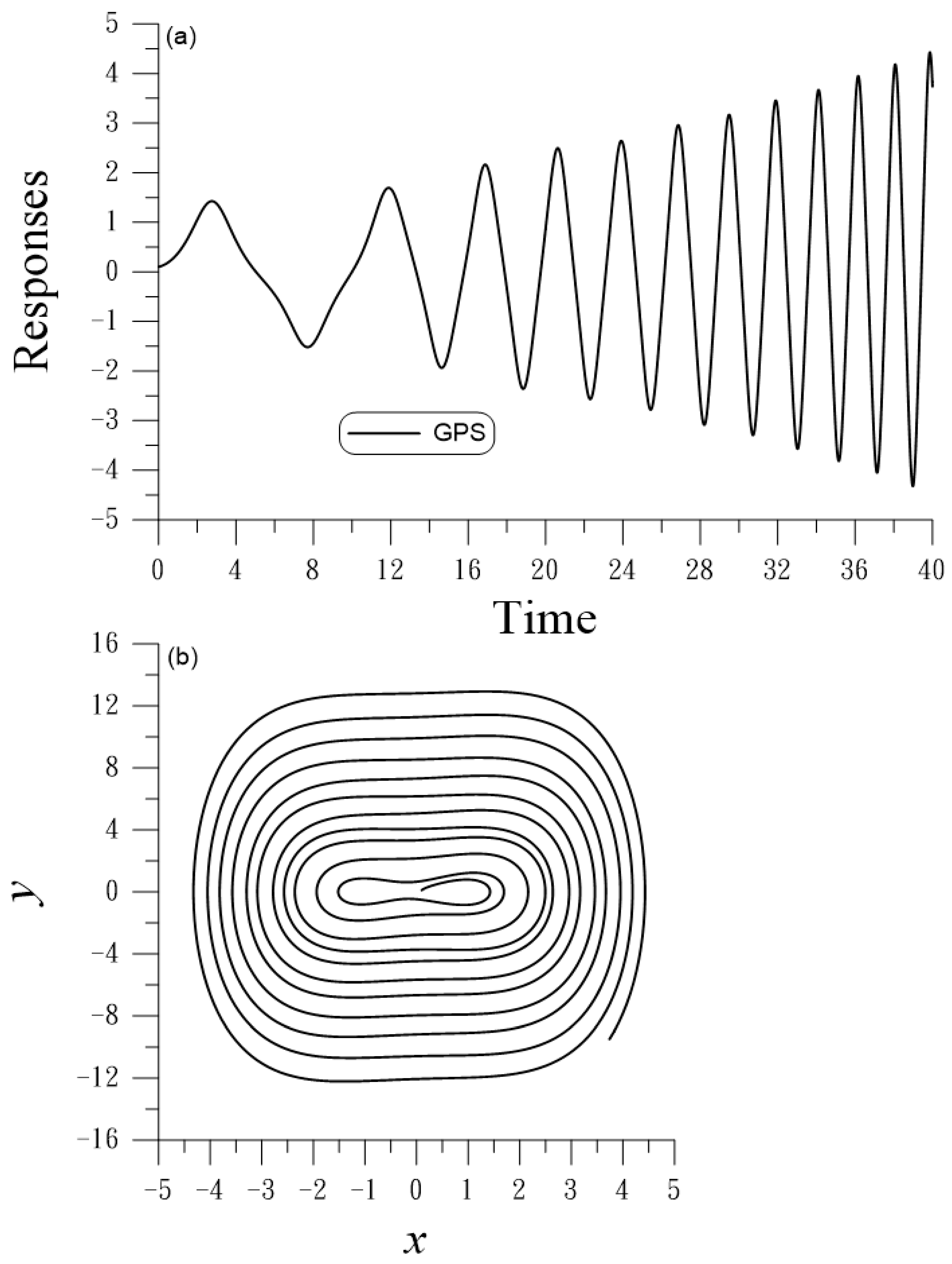
4. The GPS for a Duffing–van der Pol Oscillator

In this Section, we extend the GPS to
x ¨ ( t ) + [ γ + η x 2 ( t ) ] x ˙ ( t ) + α x ( t ) + β x 3 ( t ) = f ( t ) ,
which is a Duffing–van der Pol oscillator [69,70]. We apply the GPS to solve this problem but replacing  γ  in Equations (48) and (49) by  γ + η x ¯ k 2 .
For the special case of Equation (50) with  α = 3 / η 2 γ = 4 / η β = 1 , and  f ( t ) = 0 , it is one of the first kind Abel equations. Chandrasekar et al. [71] showed that Equation (50) can be transformed as
w ( z ) η 2 2 w 2 ( z ) w ( z ) = 0 ,
where
z : = e 2 t / η , w : = x e t / η .
Then, a particular solution is available:
x ( t ) = 3 η t 0 e 2 t / η 1 ,
where  t 0 > 1  is an arbitrary constant. If  t 0  is given, then
x ( 0 ) = 3 η t 0 1 , x ˙ ( 0 ) = 3 t 0 η 2 ( t 0 1 ) 3 / 2 .
If  x ( 0 )  is given, then, we have
t 0 = 1 + 3 η 2 x 2 ( 0 ) , x ˙ ( 0 ) = 3 t 0 η 2 ( t 0 1 ) 3 / 2 .
Mukherjee et al. [69] applied the differential transform method (DTM) using  x ( 0 ) = 0.288675134595  ( t 0 = 5 ) and  η = 3 . Using Equation (55), we can obtain  t 0  and  x ˙ ( 0 ) . GPS is compared with the DTM solution as follows:
x D T M = 0.28868 + 0.120281305 t 0.080187536 t 2 0.019916649 t 3 0.02341443 t 4 0.019687577 t 5 0.010351679 t 6 .
Table 1 compares the results provided by Mukherjee et al. [69] with the present results computed by GPS with  h = 0.01 . With the maximum error of  4.7 × 10 8 , GPS is more accurate than the DTM.
In Figure 7, we compare two responses of Duffing–van der Pol oscillators under a periodic force  f = f 0 sin ( ω t ) . We compute the response over a time interval of  t [ 0 , 1000 ]  for parameters  γ = 0.02 α = 1 β = 0.5 f 0 = 0.4 , and  ω = 1.5 , and with time stepsize  h = 0.01 . However, under a slight difference of  η = 0.0395  and  η = 0.04 , the responses as shown in Figure 7a,b are quite different. In Figure 8, we plot the Poincar e ´  section of the Duffing–van der Pol oscillator, overall 10,000 periods, under parameters  γ = 0.05 η = 0.01 α = 1 β = 0.2 f 0 = 0.4 , and  ω = 2.5 .

5. Two Coupled Duffing Equations

5.1. Hamiltonian Form

In this Section, we extend the AEPS to solve the two coupled Duffing equations:
m 1 q ¨ 1 ( t ) + c 1 q ˙ 1 ( t ) + k 1 q 1 ( t ) + β 1 q 1 3 ( t ) + c 2 [ q ˙ 1 ( t ) q ˙ 2 ( t ) ] + k 2 [ q 1 ( t ) q 2 ( t ) ] + β 2 [ q 1 ( t ) q 2 ( t ) ] 3 = f 1 ( t ) ,
m 2 q ¨ 2 ( t ) c 2 [ q ˙ 1 ( t ) q ˙ 2 ( t ) ] k 2 [ q 1 ( t ) q 2 ( t ) ] β 2 [ q 1 ( t ) q 2 ( t ) ] 3 = f 2 ( t ) .
For the energy-preserving scheme, we consider the undamped and unforced coupled Duffing equations:
m 1 q ¨ 1 ( t ) + k 1 q 1 ( t ) + β 1 q 1 3 ( t ) + k 2 [ q 1 ( t ) q 2 ( t ) ] + β 2 [ q 1 ( t ) q 2 ( t ) ] 3 = 0 ,
m 2 q ¨ 2 ( t ) k 2 [ q 1 ( t ) q 2 ( t ) ] β 2 [ q 1 ( t ) q 2 ( t ) ] 3 = 0 .
Taking the product of the above equations with  q ˙ 1 ( t )  and  q ˙ 2 ( t ) , respectively, summing the results and integrating, we yield
d d t m 1 2 q ˙ 1 2 + k 1 2 q 1 2 + β 1 4 q 1 4 + m 2 2 q ˙ 2 2 + k 2 2 [ q 1 q 2 ] 2 + β 2 4 [ q 1 q 2 ] 4 = 0 ,
m 1 2 q ˙ 1 2 + k 1 2 q 1 2 + β 1 4 q 1 4 + m 2 2 q ˙ 2 2 + k 2 2 [ q 1 q 2 ] 2 + β 2 4 [ q 1 q 2 ] 4 = C ,
where C is a constant determined by the initial values. Equation (62) indicates that the energy combined kinetic energy and potential energy is a constant value, which inspires us to develop an energy-preserving scheme.
First, we demonstrate that Equations (59) and (60) can be recast to a standard Hamiltonian form:
d d t q 1 q 2 p 1 p 2 = J H ,
where
p 1 = m 1 q ˙ 1 , p 2 = m 2 q ˙ 2 ,
H = 1 2 m 1 p 1 2 + 1 2 m 2 p 2 2 + k 1 2 q 1 2 + β 1 4 q 1 4 + k 2 2 [ q 1 q 2 ] 2 + β 2 4 [ q 1 q 2 ] 4 ,
J : = 0 2 I 2 I 2 0 2 ,
and denotes gradient with respect to the state variables  ( q 1 , q 2 , p 1 , p 2 ) . Many numerical methods have been developed to preserve the symplectic structure of the Hamiltonian systems, but in general, they do not preserve the energy, i.e., Hamiltonian function H.
The classical Hamiltonian system possesses the structures of symplecticity and energy preservation. There have been many successfully developed symplectic integrators which were used in the solution of a classical Hamiltonian system. But the symplectic integrator can only preserve the symplectic structure leading to the conservation of momentum, and which cannot guarantee the conservation of energy for the non-quadratic type Hamiltonian system. Instead of developing the symplectic integrator for the Duffing oscillators system, we are more interested in preserving the energy by developing an automatically energy-preserving scheme.

5.2. Lie-Type Forms

We propose a new approach to preserve the energy. For this purpose, we consider four possible cases (A)  β 1 > 0  and  β 2 > 0 , (B)  β 1 > 0  and  β 2 < 0 , (C)  β 1 < 0  and  β 2 > 0 , and (D)  β 1 < 0  and  β 2 < 0 .
Case (A):  β 1 > 0  and  β 2 > 0 . We let
x ˙ 1 : = m 1 q ˙ 1 ,
x ˙ 2 : = m 2 q ˙ 2 ,
y 1 : = β 1 2 q 1 2 + k 1 β 1 ,
y 2 : = β 2 2 ( q 1 q 2 ) 2 + k 2 β 2 ,
and Equation (62) can be written as
x ˙ 1 2 + x ˙ 2 2 + y 1 2 + y 2 2 = 2 C + k 1 2 2 β 1 + k 2 2 2 β 2 .
With the help from Equations (59), (60) and (67)–(70), we can derive
y ˙ 1 = 2 β 1 m 1 q 1 x ˙ 1 ,
y ˙ 2 = 2 β 2 m 1 ( q 1 q 2 ) x ˙ 1 2 β 2 m 2 ( q 1 q 2 ) x ˙ 2 ,
x ¨ 1 = 2 β 1 m 1 q 1 y 1 2 β 2 m 1 ( q 1 q 2 ) y 2 ,
x ¨ 2 = 2 β 2 m 2 ( q 1 q 2 ) y 2 .
Equations (72)–(75) can be written as
d d t y 1 y 2 x ˙ 1 x ˙ 2 = A y 1 y 2 x ˙ 1 x ˙ 2 ,
where
A : = 0 0 2 β 1 m 1 q 1 0 0 0 2 β 2 m 1 ( q 1 q 2 ) 2 β 2 m 2 ( q 1 q 2 ) 2 β 1 m 1 q 1 2 β 2 m 1 ( q 1 q 2 ) 0 0 0 2 β 2 m 2 ( q 1 q 2 ) 0 0
is skew symmetric, and the resulting Lie-group is  S O ( 4 ) .
Case (B):  β 1 > 0  and  β 2 < 0 . We let
x ˙ 1 : = m 1 q ˙ 1 ,
x ˙ 2 : = m 2 q ˙ 2 ,
y 1 : = β 1 2 q 1 2 + k 1 β 1 ,
y 2 : = β 2 2 ( q 1 q 2 ) 2 + k 2 β 2 .
In Equation (76), we have
A = 0 0 2 β 1 m 1 q 1 0 0 0 2 β 2 m 1 ( q 1 q 2 ) 2 β 2 m 2 ( q 1 q 2 ) 2 β 1 m 1 q 1 2 β 2 m 1 ( q 1 q 2 ) 0 0 0 2 β 2 m 2 ( q 1 q 2 ) 0 0 ,
where the constraint is
x ˙ 1 2 + x ˙ 2 2 + y 1 2 y 2 2 = 2 C + k 1 2 2 β 1 + k 2 2 2 β 2 ,
which is a pseudo-sphere in the pseudo-Euclidean space  R 3 , 1 . Because  A  satisfies
A T g + g A = 0 ,
g : = 1 0 0 0 0 1 0 0 0 0 1 0 0 0 0 1 ,
the resulting Lie-group is  S O ( 3 , 1 ) .
Case (C):  β 1 < 0  and  β 2 > 0 . We let
x ˙ 1 : = m 1 q ˙ 1 ,
x ˙ 2 : = m 2 q ˙ 2 ,
y 1 : = β 1 2 q 1 2 + k 1 β 1 ,
y 2 : = β 2 2 ( q 1 q 2 ) 2 + k 2 β 2 .
In terms of Equation (76),  A  is given by
A = 0 0 2 β 1 m 1 q 1 0 0 0 2 β 2 m 1 ( q 1 q 2 ) 2 β 2 m 2 ( q 1 q 2 ) 2 β 1 m 1 q 1 2 β 2 m 1 ( q 1 q 2 ) 0 0 0 2 β 2 m 2 ( q 1 q 2 ) 0 0 ,
where the constraint is
x ˙ 1 2 + x ˙ 2 2 y 1 2 + y 2 2 = 2 C + k 1 2 2 β 1 + k 2 2 2 β 2 .
Because  A  satisfies Equation (84) with
g : = 1 0 0 0 0 1 0 0 0 0 1 0 0 0 0 1 ,
the resulting Lie-group is  S O ( 3 , 1 ) .
Case (D):  β 1 < 0  and  β 2 < 0 . We let
x ˙ 1 : = m 1 q ˙ 1 ,
x ˙ 2 : = m 2 q ˙ 2 ,
y 1 : = β 1 2 q 1 2 + k 1 β 1 ,
y 2 : = β 2 2 ( q 1 q 2 ) 2 + k 2 β 2 .
We have Equation (76) but with
A = 0 0 2 β 1 m 1 q 1 0 0 0 2 β 2 m 1 ( q 1 q 2 ) 2 β 2 m 2 ( q 1 q 2 ) 2 β 1 m 1 q 1 2 β 2 m 1 ( q 1 q 2 ) 0 0 0 2 β 2 m 2 ( q 1 q 2 ) 0 0 ,
where the constraint is
x ˙ 1 2 + x ˙ 2 2 y 1 2 y 2 2 = 2 C + k 1 2 2 β 1 + k 2 2 2 β 2 ,
which is a pseudo-sphere in the pseudo-Euclidean space  R 2 , 2 . Because  A  satisfies Equation (84) with
g : = 1 0 0 0 0 1 0 0 0 0 1 0 0 0 0 1 ,
the resulting Lie-group is  S O ( 2 , 2 ) .

5.3. Automatically Energy-Preserving Scheme

For deriving an AEPS for Equations (59) and (60), we develop the numerical method from Equation (76) to compute a solution. We only consider the case of  β 1 > 0  and  β 2 > 0 . Other cases can be worked on similarly.
Accordingly, we can develop an implicit scheme based on  S O ( 4 )  for the integration of Equations (59) and (60), of which we have
A ¯ k : = 0 0 2 β 1 m 1 q ¯ 1 k 0 0 0 2 β 2 m 1 ( q ¯ 1 k q ¯ 2 k ) 2 β 2 m 2 ( q ¯ 1 k q ¯ 2 k ) 2 β 1 m 1 q ¯ 1 k 2 β 2 m 1 ( q ¯ 1 k q ¯ 2 k ) 0 0 0 2 β 2 m 2 ( q ¯ 1 k q ¯ 2 k ) 0 0 .
The corresponding  G k : = exp ( h A ¯ k )  is derived in Appendix A.
This scheme AEPS is implicit, which requires an iteration to determine the value of  ( y 1 k + 1 , y 2 k + 1 , z 1 k + 1 : = x ˙ 1 k + 1 , z 2 k + 1 : = x ˙ 2 k + 1 )  at the next time step, which is summarized as follows.
(i)
We give  0 θ 1 , h ε  and initial values, and compute  ( y 1 0 , y 2 0 , z 1 0 : = x ˙ 1 0 , z 2 0 : = x ˙ 2 0 )  by Equations (67)–(70).
(ii)
We perform  k = 0 , 1 ,  for
q 1 k + 1 = q 1 k + h q ˙ 1 k , q ˙ 1 k + 1 = q ˙ 1 k h m 1 [ k 1 q 1 k + β 1 ( q 1 k ) 3 + k 2 ( q 1 k q 2 k ) + β 2 ( q 1 k q 2 k ) 3 ] , q 2 k + 1 = q 2 k + h q ˙ 2 k , q ˙ 2 k + 1 = q ˙ 2 k + h m 2 [ k 2 ( q 1 k q 2 k ) + β 2 ( q 1 k q 2 k ) 3 ] , z 1 k + 1 = m 1 q ˙ 1 k + 1 , z 2 k + 1 = m 2 q ˙ 2 k + 1 , y 1 k + 1 = β 1 2 ( q 1 k + 1 ) 2 + k 1 β 1 , y 2 k + 1 = β 2 2 ( q 1 k + 1 q 2 k + 1 ) 2 + k 2 β 2 .
(iii)
We iteratively solve the new  ( y 1 k + 1 , y 2 k + 1 , z 1 k + 1 , z 2 k + 1 )  by
q ¯ 1 k = ( 1 θ ) q 1 k + θ q 1 k + 1 , q ¯ 2 k = ( 1 θ ) q 2 k + θ q 2 k + 1 , Compute G k by   Equation ( A20 ) , y ^ 1 k + 1 y ^ 2 k + 1 z ^ 1 k + 1 z ^ 2 k + 1 = G k y 1 k y 2 k z 1 k z 2 k , q 1 k + 1 = ± 2 β 1 y ^ 1 k + 1 k 1 β 1 1 / 2 , q 2 k + 1 = q 1 k + 1 ± 2 β 2 y ^ 2 k + 1 k 2 β 2 1 / 2 .
If
( y ^ 1 k + 1 y 1 k + 1 ) 2 + ( y ^ 2 k + 1 y 2 k + 1 ) 2 + ( z ^ 1 k + 1 z 1 k + 1 ) 2 + ( z ^ 2 k + 1 z 2 k + 1 ) 2 < ε ,
then we proceed to (ii) for the next time step; otherwise, we let  y 1 k + 1 = y ^ 1 k + 1 y 2 k + 1 = y ^ 2 k + 1 z 1 k + 1 = z ^ 1 k + 1  and  z 2 k + 1 = z ^ 2 k + 1 , and proceed to (iii) for executing Equation (102).
We consider Equations (59) and (60) under initial conditions  q 1 ( 0 ) = 0.1 q ˙ 1 ( 0 ) = 0.1 ,   q 2 ( 0 ) = 0.1  and  q ˙ 2 ( 0 ) = 0 , and with the same parameter values,  m 1 = 2 m 2 = 1 k 1 = 5 k 2 = 2 β 1 = 0.5  and  β 2 = 0.2 .
We solve the problem using the AEPS with  h = 0.001  and  ε = 10 8 , and plot the time histories and phase portraits in Figure 9 in the time range of  t [ 0 , 10 ] . Even under a stringent convergence criterion with  ε = 10 8 , the AEPS converges very fast with 2 iterations at each time step as shown in Figure 9i. The value of  C = 0.0035005  is compared with that computed by the AEPS, of which the error is shown in Figure 9j. It can be seen that the capability in the preservation of energy of the AEPS is good.

5.4. Group-Preserving Scheme for Damped and Forced System

Now, a group-preserving scheme (GPS) for the solution of Equations (57) and (58) is derived. In terms of  ( y 1 , y 2 , x ˙ 1 , x ˙ 2 ) , we can write
d d t y 1 y 2 x ˙ 1 x ˙ 2 = A y 1 y 2 x ˙ 1 x ˙ 2 + 0 0 1 m 1 f 1 ( t ) 1 m 2 f 2 ( t ) ,
where
A : = 0 0 2 β 1 m 1 q 1 0 0 0 2 β 2 m 1 ( q 1 q 2 ) 2 β 2 m 2 ( q 1 q 2 ) 2 β 1 m 1 q 1 2 β 2 m 1 ( q 1 q 2 ) c 1 + c 2 m 1 c 2 m 1 m 2 0 2 β 2 m 2 ( q 1 q 2 ) c 2 m 1 m 2 c 2 m 2 .
By applying the Trapezoidal rule on the integral term, we can derive
y 1 k + 1 y 2 k + 1 z 1 k + 1 z 2 k + 1 = G k y 1 k y 2 k z 1 k z 2 k + τ 0 0 1 m 1 f 1 ( t k + 1 ) 1 m 2 f 2 ( t k + 1 ) + τ G k 0 0 1 m 1 f 1 ( t k ) 1 m 2 f 2 ( t k ) ,
where  τ = h / 2 , and
G k = ( I 4 τ A ¯ k ) 1 ( I 4 + τ A ¯ k ) ,
( I 4 τ A ¯ k ) 1 = I 2 + U ( D V U ) 1 V U ( D V U ) 1 ( D V U ) 1 V ( D V U ) 1 ,
in which the  2 × 2  matrices  U V  and  D  are given by
I 2 U V D : = 1 0 τ 2 β 1 m 1 q ¯ 1 k 0 0 1 τ 2 β 2 m 1 ( q ¯ 1 k q ¯ 2 k ) τ 2 β 2 m 2 ( q ¯ 1 k q ¯ 2 k ) τ 2 β 1 m 1 q ¯ 1 k τ 2 β 2 m 1 ( q ¯ 1 k q ¯ 2 k ) 1 + τ ( c 1 + c 2 ) m 1 τ c 2 m 1 m 2 0 τ 2 β 2 m 2 ( q ¯ 1 k q ¯ 2 k ) τ c 2 m 1 m 2 1 + τ c 2 m 2 .
Therefore, the GPS for Equations (57) and (58) is an iterative algorithm to determine the value of  ( y 1 k + 1 , y 2 k + 1 , z 1 k + 1 : = x ˙ 1 k + 1 , z 2 k + 1 : = x ˙ 2 k + 1 )  at the next time step, which is summarized as follows.
(i)
We give  0 θ 1 , initial values at initial time  t 0 = 0  and time stepsize h, and compute the initial values of  ( y 1 0 , y 2 0 , z 1 0 : = x ˙ 1 0 , z 2 0 : = x ˙ 2 0 )  by Equations (67)–(70).
(ii)
For  k = 0 , 1 , , we repeat
q 1 k + 1 = q 1 k + h q ˙ 1 k , q ˙ 1 k + 1 = q ˙ 1 k h m 1 [ k 1 q 1 k + β 1 ( q 1 k ) 3 + k 2 ( q 1 k q 2 k ) + β 2 ( q 1 k q 2 k ) 3 ( c 1 + c 2 ) q ˙ 1 k + c 2 q ˙ 2 k + f 1 ( t k ) ] , q 2 k + 1 = q 2 k + h q ˙ 2 k , q ˙ 2 k + 1 = q ˙ 2 k + h m 2 [ k 2 ( q 1 k q 2 k ) + β 2 ( q 1 k q 2 k ) 3 + c 2 q ˙ 1 k c 2 q ˙ 2 k + f 2 ( t k ) ] , z 1 k + 1 = m 1 q ˙ 1 k + 1 , z 2 k + 1 = m 2 q ˙ 2 k + 1 , y 1 k + 1 = β 1 2 ( q 1 k + 1 ) 2 + k 1 β 1 , y 2 k + 1 = β 2 2 ( q 1 k + 1 q 2 k + 1 ) 2 + k 2 β 2 .
(iii)
The new  ( y 1 k + 1 , y 2 k + 1 , z 1 k + 1 , z 2 k + 1 )  is iterated by
q ¯ 1 k = ( 1 θ ) q 1 k + θ q 1 k + 1 , q ¯ 2 k = ( 1 θ ) q 2 k + θ q 2 k + 1 , We compute G k by Equation ( 107 ) : y ^ 1 k + 1 y ^ 2 k + 1 z ^ 1 k + 1 z ^ 2 k + 1 = G k y 1 k y 2 k z 1 k z 2 k + τ 0 0 f 1 ( t k + 1 ) m 1 f 2 ( t k + 1 ) m 2 + τ G k 0 0 1 m 1 f 1 ( t k ) 1 m 2 f 2 ( t k ) , q 1 k + 1 = ± 2 β 1 y ^ 1 k + 1 k 1 β 1 1 / 2 , q 2 k + 1 = q 1 k + 1 ± 2 β 2 y ^ 2 k + 1 k 2 β 2 1 / 2 .
If
( y ^ 1 k + 1 y 1 k + 1 ) 2 + ( y ^ 2 k + 1 y 2 k + 1 ) 2 + ( z ^ 1 k + 1 z 1 k + 1 ) 2 + ( z ^ 2 k + 1 z 2 k + 1 ) 2 < ε ,
then we proceed to (ii) for the next time step; otherwise, we let  y 1 k + 1 = y ^ 1 k + 1 y 2 k + 1 = y ^ 2 k + 1 z 1 k + 1 = z ^ 1 k + 1  and  z 2 k + 1 = z ^ 2 k + 1 , and proceed to (iii) for conducting computations in Equation (111).
In Figure 10, we plot the responses of the coupled Duffing oscillator under  m 1 = 0.5 m 2 = 1 k 1 = 5 k 2 = 2 m 1 = 0.5 m 2 = 1 β 1 = 1 β 2 = 2 c 1 = 0.2  and  c 2 = 0.3 , where the external forces are given by  f 1 ( t ) = 0.7 cos 1.2 t  and  f 2 ( t ) = 0.7 sin 1.2 t . Even under a stringent convergence criterion with  ε = 10 7 , the GPS converges very fast with 3 iterations at each time step as shown in Figure 10i. Under the following parameters,  m 1 = 0.5 m 2 = 1 k 1 = 5 k 2 = 2 m 1 = 0.5 m 2 = 1 β 1 = 1 β 2 = 2 c 1 = 0.2  and  c 2 = 0.03 f 1 ( t ) = 1.5 cos 2.5 t  and  f 2 ( t ) = 1.5 sin 2.5 t , we plot the Poincar e ´  sections in Figure 11 with 8000 periodic points in total.

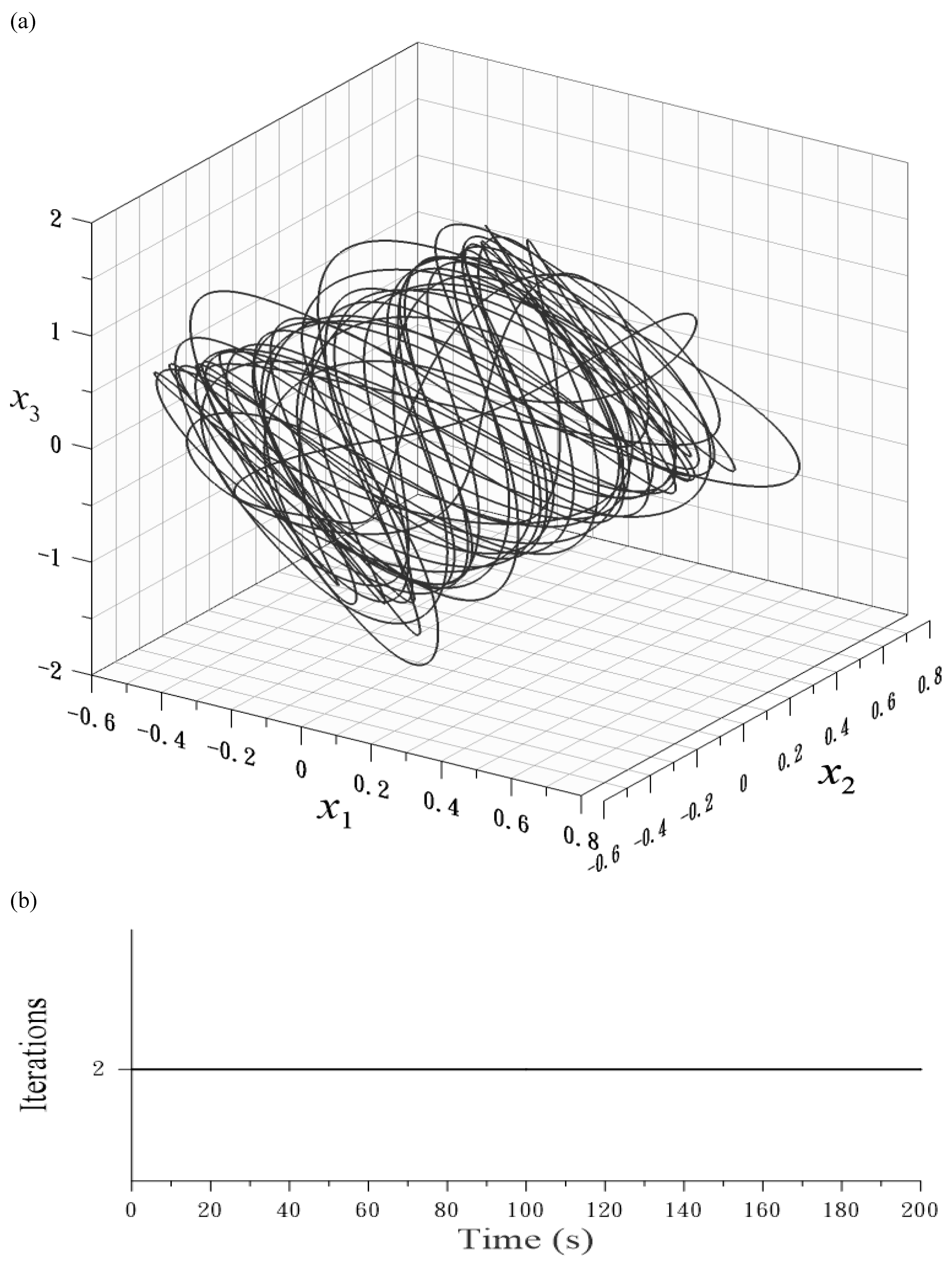
6. Three Coupled Duffing Equations

In this Section, we extend the GPS to solve the three coupled Duffing equations:
m 1 q ¨ 1 ( t ) + c 1 q ˙ 1 ( t ) + k 1 q 1 ( t ) + β 1 q 1 3 ( t ) + c 2 [ q ˙ 1 ( t ) q ˙ 2 ( t ) ] + k 2 [ q 1 ( t ) q 2 ( t ) ] + β 2 [ q 1 ( t ) q 2 ( t ) ] 3 = 0 , m 2 q ¨ 2 ( t ) c 2 [ q ˙ 1 ( t ) q ˙ 2 ( t ) ] k 2 [ q 1 ( t ) q 2 ( t ) ] β 2 [ q 1 ( t ) q 2 ( t ) ] 3 + c 3 [ q ˙ 2 ( t ) q ˙ 3 ( t ) ] + k 3 [ q 2 ( t ) q 3 ( t ) ] + β 3 [ q 2 ( t ) q 3 ( t ) ] 3 = 0 , m 3 q ¨ 3 c 3 [ q ˙ 2 ( t ) q ˙ 3 ( t ) ] k 3 [ q 2 ( t ) q 3 ( t ) ] β 3 [ q 2 ( t ) q 3 ( t ) ] 3 = f 0 cos ω t .
Let us consider the undamped and unforced three coupled Duffing equations such that we have
m 1 2 q ˙ 1 2 + k 1 2 q 1 2 + β 1 4 q 1 4 + m 2 2 q ˙ 2 2 + k 2 2 [ q 1 q 2 ] 2 + β 2 4 [ q 1 q 2 ] 4 + m 3 2 q ˙ 3 2 + k 3 2 [ q 2 q 3 ] 2 + β 3 4 [ q 2 q 3 ] 4 = C ,
where C is a constant determined by the initial values.
For Equation (114), we have four pseudo-sphere realizations depending on the values of  β i , i = 1 , 2 , 3 . We only consider  β 1 > 0 β 2 > 0  and  β 3 < 0  as a demonstrative case, and the other cases can be examined similarly. We let
x ˙ 1 : = m 1 q ˙ 1 , x ˙ 2 : = m 2 q ˙ 2 , x ˙ 3 : = m 3 q ˙ 3 , y 1 : = β 1 2 q 1 2 + k 1 β 1 , y 2 : = β 2 2 ( q 1 q 2 ) 2 + k 2 β 2 , y 3 : = β 3 2 ( q 2 q 3 ) 2 + k 3 β 3 ,
and Equation (114) can be written as
x ˙ 1 2 + x ˙ 2 2 + x ˙ 3 2 + y 1 2 + y 2 2 y 3 2 = 2 C + k 1 2 2 β 1 + k 2 2 2 β 2 + k 3 2 2 β 3 ,
where we suppose that  β 1 > 0 β 2 > 0  and  β 3 < 0 . Equation (116) indicates that the constraint is a pseudo-sphere in the pseudo-Euclidean space  R 5 , 1 .
In terms of  ( y 1 , y 2 , y 3 , x ˙ 1 , x ˙ 2 , x ˙ 3 ) , we can write Equation (113) as a system:
d d t y 1 y 2 y 3 x ˙ 1 x ˙ 2 x ˙ 3 = A y 1 y 2 y 3 x ˙ 1 x ˙ 2 x ˙ 3 + 0 0 0 0 0 f 0 cos ω t m 3 ,
where
A : = 0 0 0 2 β 1 m 1 q 1 0 0 0 0 0 2 β 2 m 1 ( q 1 q 2 ) 2 β 2 m 2 ( q 1 q 2 ) 0 0 0 0 0 2 β 3 m 2 ( q 2 q 3 ) 2 β 3 m 3 ( q 2 q 3 ) 2 β 1 m 1 q 1 2 β 2 m 1 ( q 1 q 2 ) 0 c 1 + c 2 m 1 c 2 m 1 m 2 0 0 2 β 2 m 2 ( q 1 q 2 ) 2 β 3 m 2 ( q 2 q 3 ) c 2 m 1 m 2 c 2 + c 3 m 2 c 3 m 2 m 3 0 0 2 β 3 m 3 ( q 2 q 3 ) 0 c 3 m 2 m 3 c 3 m 3 .
For the special case with  c i = 0 , i = 1 , 2 , 3 , the above  A  is a Lie-algebra element of the type  s o ( p , q )  with  p = 5  and  q = 1 . Depending on the values of  β i , i = 1 , 2 , 3  there are four Lie-algebras:  s o ( 3 , 3 )  ( β 1 < 0 β 2 < 0  and  β 3 < 0 ),  s o ( 4 , 2 )  ( β 1 > 0 β 2 < 0  and  β 3 < 0 β 1 < 0 β 2 > 0  and  β 3 < 0 , and  β 1 < 0 β 2 < 0  and  β 3 > 0 ),  s o ( 5 , 1 )  ( β 1 > 0 β 2 > 0  and  β 3 < 0 β 1 > 0 β 2 < 0  and  β 3 > 0 , and  β 1 < 0 β 2 > 0  and  β 3 > 0 ),  s o ( 6 )  ( β 1 > 0 β 2 > 0  and  β 3 > 0 ). Correspondingly, the resulting Lie-groups  G  have four types:  S O ( 3 , 3 ) S O ( 4 , 2 ) S O ( 5 , 1 )  and  S O ( 6 ) , depending on parameters  β 1 β 2  and  β 3  of nonlinear springs.
The numerical process is similar to that given in Section 5. First, we consider an undamped and unforced case with  c 1 = c 2 = c 3 = 0 m 1 = 2 m 2 = 1 m 3 = 0.5 k 1 = 2 k 2 = 3 k 3 = 1 β 1 = 0.2 β 2 = 0.5 , and  β 3 = 0.2 . However, under  ε = 10 8 , the number of iterations is two, as shown in Figure 12a, while the error of energy as shown in Figure 12b is very small in the order of  10 12 . Then, we consider a damped and forced case with  c 1 = 0.05 c 2 = 0.02 c 3 = 0.02 f 0 = 0.2  and  ω = 1.5 . Other parameters are the same as those in the above. In Figure 13a, we plot the three-dimensional orbit and the number of iterations in Figure 13b. Finally, for the three hardening springs with  β 1 = 0.2 β 2 = 0.5 , and  β 3 = 0.7 , we plot the phase portraits and the number of iterations in Figure 14, where  f 0 = 0.5  and  ω = 0.2 .
For the purpose of comparison, we also applied the fourth-order Runge–Kutta method (RK4) to solve an undamped and unforced case to a large final time  t f = 500 . The step size is taken to be  h = 0.005 . In Figure 15, the errors of energy obtained by RK4 and AEPS are compared. Obviously, the capability of AEPS to preserve the energy is better than that of RK4 by several orders of magnitude. When a very small value in the order of  10 13  was achieved by AEPS, for RK4, the error was in the order of  10 10 .
A practical implication is that when the AEPS can sustain the energy automatically, it is more suitable to observe the long-term free vibration behavior of nonlinear Duffing oscillators, which are used to model many engineering mechanical vibration systems. Even with a wide gap in the linear frequencies of the coupled Duffing oscillator system with  k 1 = 20 k 2 = 10 k 3 = 1 , AEPS were still performed well to preserve the energy as shown in Figure 16 to compare with that obtained by RK4.
When the number of the components of the coupled Duffing oscillators system is increased to n, the drawback is that it needs more time to analytically construct the transformations between  2 n  variables, and the dimension of the Lie-group matrix  G k  is increased to  ( n + 1 ) × ( n + 1 ) .

7. Conclusions

For the undamped and unforced Duffing equations, we transformed the invariant condition for the conservation of energy into a pseudo-sphere in the pseudo-Euclidean space  R p , q  with a signature  ( p , q ) . The resulting new ODEs system admits an  S O ( p , q )  Lie-group symmetry with a local Lie-algebra,  A s o ( p , q ) . Then, we developed a Lie-group  S O ( p , q )  scheme to preserve the pseudo-sphere invariant, which rendered the energy of the Duffing system to be conserved automatically. Evaluating the high performance of the developed automatically energy-preserving scheme (AEPS) for the numerical solutions of coupled Duffing equations, we offered examples to show its high accuracy by comparison with the power series solution and with an exact solution of the Duffing–van der Pol equation, of which the accuracy can arrive to the fourth order. The computational cost is quite low, because the preservation of energy is automatic without needing iteration, which is different from other energy-conserving methods. However, to enhance the accuracy of the numerical integration, we adopted the mid-point value to compute the Lie-algebra and then the Lie-group, of which a few iterations in Part (iii) of each algorithm are required. Then, we developed group-preserving schemes for damped and forced multi-coupled Duffing equations, and some numerical results and Poincar e ´  sections were given and displayed. Owing to the damped term, the resulting Lie-group is of the dilation type, denoted as  D S O ( p , q ) . The corresponding group-preserving schemes exhibited the same advantage of the Lie-group, which can be used to depict the long term behavior of damped and forced multi-coupled Duffing oscillators. The methodologies including quadratic forms, Lie-algebras and Lie-groups are novel, appearing for the first time to investigate the nonlinear vibrational behaviors of multi-coupled Duffing oscillators.

Author Contributions

Conceptualization, C.-L.K. and C.-W.C.; Methodology, C.-S.L. and C.-W.C.; Software, C.-S.L. and C.-W.C.; Validation, C.-S.L. and C.-W.C.; Formal analysis, C.-S.L. and C.-W.C.; Investigation, C.-S.L. and C.-W.C.; Resources, C.-W.C.; Data curation, C.-S.L.; Writing—original draft, C.-S.L.; Writing—review and editing, C.-W.C.; Visualization, C.-L.K. and C.-W.C.; Supervision, C.-W.C.; Project administration, C.-W.C. All authors have read and agreed to the published version of the manuscript.

Funding

This research received no external funding.

Institutional Review Board Statement

Not applicable.

Informed Consent Statement

Not applicable.

Data Availability Statement

The data presented in this study are available on request from the corresponding authors. The data are not publicly available due to restrictions privacy.

Conflicts of Interest

The authors declare no conflict of interest.

Appendix A

In this Appendix, we derive state transition matrix  G  corresponding to  A  given in Equation (100). Upon letting
a : = 2 β 1 m 1 q ¯ 1 k ,
b : = 2 β 2 m 1 ( q ¯ 1 k q ¯ 2 k ) ,
c : = 2 β 2 m 2 ( q ¯ 1 k q ¯ 2 k ) ,
we can obtain the following ODEs system:
z ˙ 1 = a z 3 , z ˙ 2 = b z 3 c z 4 , z ˙ 3 = a z 1 b z 2 , z ˙ 4 = c z 2 .
Through some derivations, we can obtain
d 4 z 1 d t 4 + ( a 2 + b 2 + c 2 ) z ¨ 1 + a 2 c 2 z 1 = 0 ,
of which the general solution is
z 1 = k 1 cos ω 1 t + k 2 sin ω 1 t + k 3 cos ω 2 t + k 4 sin ω 2 t ,
where
a 0 : = a 2 + b 2 + c 2 ,
b 0 : = a 2 c 2 ,
ω 1 : = a 0 + a 0 2 4 b 0 2 1 / 2 ,
ω 2 = a 0 ω 1 2 = a 0 a 0 2 4 b 0 2 1 / 2 .
Similarly, we can derive
z 2 = c 0 k 1 cos ω 1 t + c 0 k 2 sin ω 1 t + d 0 k 3 cos ω 2 t + d 0 k 4 sin ω 2 t ,
z 3 = ω 1 a k 1 sin ω 1 t + ω 1 a k 2 cos ω 1 t ω 2 a k 3 sin ω 2 t + ω 2 a k 4 cos ω 2 t ,
z 4 = e 0 k 1 sin ω 1 t + e 0 k 2 cos ω 1 t f 0 k 3 sin ω 2 t + f 0 k 4 cos ω 2 t ,
where
c 0 = ω 1 2 a b a b ,
d 0 = ω 2 2 a b a b ,
e 0 = b ω 1 a c c 0 ω 1 c ,
f 0 = b ω 2 a c d 0 ω 2 c .
In terms of the following matrix:
H ( t ) : = cos ω 1 t sin ω 1 t cos ω 2 t sin ω 2 t c 0 cos ω 1 t c 0 sin ω 1 t d 0 cos ω 2 t d 0 sin ω 2 t ω 1 a sin ω 1 t ω 1 a cos ω 1 t ω 2 a sin ω 2 t ω 2 a cos ω 2 t e 0 sin ω 1 t e 0 cos ω 1 t f 0 sin ω 2 t f 0 cos ω 2 t ,
Equations (A6) and (A11)–(A13) can be written as
z 1 ( t ) z 2 ( t ) z 3 ( t ) z 4 ( t ) = H ( t ) k 1 k 2 k 3 k 4 .
Finally, the state transition matrix can be written as
G ( t ) = H ( t ) H 1 ( 0 ) = cos ω 1 t sin ω 1 t cos ω 2 t sin ω 2 t c 0 cos ω 1 t c 0 sin ω 1 t d 0 cos ω 2 t d 0 sin ω 2 t ω 1 a sin ω 1 t ω 1 a cos ω 1 t ω 2 a sin ω 2 t ω 2 a cos ω 2 t e 0 sin ω 1 t e 0 cos ω 1 t f 0 sin ω 2 t f 0 cos ω 2 t d 0 d 0 c 0 1 c 0 d 0 0 0 0 0 a ω 1 + a ω 2 q 0 ω 1 2 ω 2 q 0 e 0 ω 1 c 0 c 0 d 0 1 d 0 c 0 0 0 0 0 a q 0 ω 1 1 q 0 e 0 ,
where
q 0 = f 0 e 0 ω 2 ω 1 .

References

  1. Farkas, M. Periodic Motions; Springer: New York, NY, USA, 1994. [Google Scholar]
  2. Cvetićanin, L. Ninety years of Duffing’s equation. Theor. Appl. Mech. 2013, 40, 49–63. [Google Scholar]
  3. Hu, N.; Wen, X. The application of duffing oscillator in characteristic signal detection of early fault. J. Sound Vib. 2003, 268, 917–931. [Google Scholar]
  4. Suhardjo, J.; Spencer, B.F., Jr.; Sain, M.K. Non-linear optimal control of a Duffing system. Int. J. Non-Linear Mech. 1992, 27, 157–172. [Google Scholar]
  5. Wang, G.; Zhenga, W.; He, S. Estimation of amplitude and phase of a weak signal by using the property of sensitive dependence on initial conditions of a nonlinear oscillator. Signal Proc. 2002, 82, 103–115. [Google Scholar]
  6. Maimistov, A.I. Some models of propagation of extremely short electromagnetic pulses in a nonlinear medium. Quantum Elect. 2000, 30, 287–304. [Google Scholar]
  7. Maimistov, A.I. Propagation of an ultimately short electromagnetic pulse in a nonlinear medium described by the fifth-order Duffing model. Opt. Spect. 2003, 30, 251–257. [Google Scholar]
  8. Zeeman, E.C. Duffing’s equation in brain modelling. Bull. Inst. Math. Appl. 1976, 12, 207–214. [Google Scholar]
  9. Donescu, P.; Virgin, L.N.; Wu, J.J. Periodic solutions of an unsymmetric oscillator including a comprehensive study of their stability characteristics. J. Sound Vib. 1996, 192, 959–976. [Google Scholar] [CrossRef]
  10. Wu, B.S.; Sun, W.P.; Lim, C.W. An analytical approximate technique for a class of strongly non-linear oscillators. Int. J. Non-Linear Mech. 2006, 41, 766–774. [Google Scholar] [CrossRef]
  11. Liu, L.; Thomas, J.P.; Dowell, E.H.; Attar, P.; Hall, K.C. A comparison of classical and high dimension harmonic balance approaches for a Duffing oscillator. J. Comput. Phys. 2006, 215, 298–320. [Google Scholar] [CrossRef]
  12. He, J.H. Variational iteration method—A kind of non-linear analytic technique: Some examples. Int. J. Non-Linear Mech. 1999, 34, 699–708. [Google Scholar] [CrossRef]
  13. Ozis, T.; Yildirim, A. A study of nonlinear oscillators with u1/3 force by He’s variational iteration method. J. Sound Vib. 2007, 306, 372–376. [Google Scholar] [CrossRef]
  14. He, J.H. A coupling method of a homotopy technique and a perturbation technique for non-linear problems. Int. J. Non-Linear Mech. 2000, 35, 37–43. [Google Scholar]
  15. Shou, D.H. The homotopy perturbation method for nonlinear oscillators. Comput. Math. Appl. 2009, 58, 2456–2459. [Google Scholar] [CrossRef]
  16. Koroglu, C.; Ozis, T. Applications of parameter-expanding method to nonlinear oscillators in which the restoring force is inversely proportional to the dependent variable or in form of rational function of dependent variable. Comput. Model. Eng. Sci. 2011, 75, 223–234. [Google Scholar]
  17. He, J.H.; Abdou, A. New periodic solutions for nonlinear evolution equations using exp-function method. Chaos Soliton Frac. 2007, 34, 1421–1429. [Google Scholar] [CrossRef]
  18. Chu, H.P.; Lo, C.Y. Application of the differential transform method for solving periodic solutions of strongly non-linear oscillators. Comput. Model. Eng. Sci. 2011, 77, 161–172. [Google Scholar]
  19. Qaisi, M.I. A power series approach for the study of periodic motion. J. Sound Vib. 1996, 196, 401–406. [Google Scholar] [CrossRef]
  20. Schovanec, L.; White, J.T. A power series method for solving initial value problems utilizing computer algebra systems. Int. J. Comput. Math. 1993, 47, 181–189. [Google Scholar] [CrossRef]
  21. Chen, Y.Z. Solution of the Duffing equation by using target function method. J. Sound Vib. 2002, 256, 573–578. [Google Scholar] [CrossRef]
  22. Yusufoglu, E. Numerical solutio of Duffing equation by the Laplace decomposition algorithm. Appl. Math. Comput. 2006, 177, 572–580. [Google Scholar]
  23. Khuri, S.A. A Laplace decomposition algorithm applied to a class of nonlinear differential equations. J. Appl. Math. 2001, 1, 141–155. [Google Scholar]
  24. Elgohary, T.A.; Dong, L.; Junkins, J.L.; Atluri, S.N. A simple, fast, and accurate time-integrator for strongly nonlinear dynamical systems. Comput. Model. Eng. Sci. 2014, 100, 249–275. [Google Scholar]
  25. Liu, C.-S.; Jhao, W.S. The power series method for a long term solution of Duffing oscillator. Commun. Numer. Anal. 2014, 2014, 1–14. [Google Scholar] [CrossRef]
  26. Dai, H.H.; Yan, Z.P.; Wang, X.C.; Yue, X.; Atluri, S.N. Collocation-based harmonic balance framework for highly accurate periodic solution of nonlinear dynamical system. Int. J. Numer. Meth. Eng. 2023, 124, 458–481. [Google Scholar] [CrossRef]
  27. Liu, C.-S.; Kuo, C.L.; Jhao, W.S. A multiple-scale power series method for solving nonlinear ordinary differential equations. Communi. Numer. Ana. 2016, 2016, 37–49. [Google Scholar]
  28. Liu, C.-S. Cone of non-linear dynamical system and group preserving schemes. Int. J. Non-Linear Mech. 2001, 36, 1047–1068. [Google Scholar] [CrossRef]
  29. Akgül, A.; Inc, M.; Hashemi, M.S. Group preserving scheme and reproducing kernel method for the Poisson–Boltzmann equation for semiconductor devices. Nonlinear Dyn. 2017, 88, 2817–2829. [Google Scholar] [CrossRef]
  30. Hashemi, M.S.; Inc, M.; Karatas, E.; Darvish, E. Numerical treatment on one-dimensional hyperbolic telegraph equation by the method of line-group preserving scheme. Eur. Phys. J. Plus 2019, 134, 153. [Google Scholar] [CrossRef]
  31. Gao, W.; Partohaghighi, M.; Baskonus, H.M.; Ghavi, S. Regarding the group preserving scheme and method of line to the numerical simulations of Klein–Gordon model. Results Phys. 2019, 15, 102555. [Google Scholar]
  32. Hashemi, M.S.; Baleanu, D.; Parto-Haghighi, M. A Lie group approach to solve the fractional poisson equation. Rom. J. Phys. 2015, 60, 1289–1297. [Google Scholar]
  33. Hashemi, M.S.; Baleanu, D.; Parto-Hghighi, M.; Darvishi, E. Solving the time fractional diffusion equation using Lie group integrator. Thermal Sci. 2015, 19 (Suppl. S1), S77–S83. [Google Scholar] [CrossRef]
  34. Abbasbandy, S.; Hashemi, M. Group preserving scheme for the cauchy problem of the laplace equation. Eng. Anal. Bound. Elem. 2011, 35, 1003–1009. [Google Scholar] [CrossRef]
  35. Hashemi, M. Numerical study of the one dimensional coupled nonlinear sine Gordon equations by a novel geometric meshless method. Eng. Comput. 2021, 37, 3397–3407. [Google Scholar] [CrossRef]
  36. Seydaoglu, M. A meshless method for Burgers’ equation using multiquadric radial basis functions with a Lie-group integrator. Mathematics 2019, 7, 113. [Google Scholar]
  37. Xu, Z.; Wu, J. MGPS: Midpoint-series group preserving scheme for discretizing nonlinear dynamics. Symmetry 2022, 35, 1003–1009. [Google Scholar]
  38. Partohaghighi, M.; Akgül, A.; Akgül, E.K.; Attia, N.; De la Sen, M.; Bayram, M. Analysis of the fractional differential equations using two different methods. Symmetry 2023, 15, 65. [Google Scholar] [CrossRef]
  39. Simo, J.C.; Tarnow, N.; Wong, K.K. Exact energy-momentum conserving algorithms and symplectic schemes 284 for nonlinear dynamics. Comp. Meth. Appl. Mech. Eng. 1992, 100, 63–116. [Google Scholar] [CrossRef]
  40. Liu, C.S. Preserving constraints of differential equations by numerical methods based on integrating factors. Comput. Model. Eng. Sci. 2006, 12, 83–107. [Google Scholar]
  41. Brugnano, L.; Iavernaro, F.; Trigiante, D. Energy- and quadratic invariants-preserving integrators based upon Gauss collocation formulae. SIAM J. Num. Anal. 2012, 50, 2897–2916. [Google Scholar] [CrossRef]
  42. Brugnano, L.; Iavernaro, F.; Trigiante, D. A two-step, fourth-order method with energy preserving properties. Comput. Phys. Commun. 2012, 183, 1860–1868. [Google Scholar]
  43. Brugnano, L.; Calvo, M.; Montijano, J.I.; Randez, L. Energy-preserving methods for Poisson systems. J. Comput. Appl. Math. 2012, 236, 3890–3904. [Google Scholar]
  44. Brugnano, L.; Iavernaro, F.; Trigiante, D. Analysis of Hamiltonian boundary value methods (HBVMs): A class of energy-preserving Runge-Kutta methods for the numerical solution of polynomial Hamiltonian systems. Commun. Nonlinear Sci. Numer. Simulat. 2015, 20, 650–667. [Google Scholar] [CrossRef]
  45. Celledoni, E.; McLachlan, R.I.; Owren, B.; Quispel, G.R.W. Energy-preserving integrators and the Structure of B-series. Found. Comp. Math. 2010, 10, 673–693. [Google Scholar] [CrossRef]
  46. Wu, X.; Wang, B.; Shi, W. Efficient energy-preserving integrators for oscillatory Hamiltonian systems. J. Comp. Phys. 2013, 235, 587–605. [Google Scholar]
  47. Hong, J.; Ji, L.; Zhang, L.; Cai, J. An energy-conserving method for stochastic Maxwell equations with multiplicative noise. J. Comput. Phys. 2017, 351, 216–229. [Google Scholar] [CrossRef]
  48. Barletti, L.; Brugnano, L.; Frasca Caccia, G.; Iavernaro, F. Energy-conserving methods for the nonlinear Schrödinger equation. Appl. Math. Comput. 2018, 318, 3–18. [Google Scholar]
  49. Umeda, A.; Wakasugi, Y.; Yoshikawa, S. Energy-conserving finite difference schemes for nonlinear wave equations with dynamic boundary conditions. Appl. Numer. Math. 2022, 171, 1–22. [Google Scholar] [CrossRef]
  50. Cheng, X.; Qin, H.; Zhang, J. Convergence of an energy-conserving scheme for nonlinear space fractional Schrödinger equations with wave operator. J. Comput. Appl. Math. 2022, 400, 113762. [Google Scholar] [CrossRef]
  51. Fu, Y.; Zhang, X.; Qin, H. An explicitly solvable energy-conserving algorithm for pitch-angle scattering in magnetized plasmas. J. Comput. Phys. 2022, 449, 110767. [Google Scholar] [CrossRef]
  52. Yang, R.; Xing, Y. Energy conserving discontinuous Galerkin method with scalar auxiliary variable technique for the nonlinear Dirac equation. J. Comput. Phys. 2022, 463, 111278. [Google Scholar] [CrossRef]
  53. Shin, J.; Lee, J.-Y. Energy conserving successive multi-stage method for the linear wave equation. J. Comput. Phys. 2022, 458, 111098. [Google Scholar]
  54. Zhang, W.; Liu, C.; Jiang, C.; Zheng, C. Arbitrary high-order linearly implicit energy-conserving schemes for the Rosenau-type equation. Appl. Math. Lett. 2023, 138, 108530. [Google Scholar]
  55. Hu, M.; Tian, J.; Sun, P.; Zhang, Z. An energy-conserving finite element method for nonlinear fourth-order wave equations. Appl. Numer. Math. 2023, 183, 333–354. [Google Scholar]
  56. Pagliantini, C.; Manzini, G.; Koshkarov, O.; Delzanno, G.L.; Roytershteyn, V. Energy-conserving explicit and implicit time integration methods for the multi-dimensional Hermite-DG discretization of the Vlasov-Maxwell equations. Comput. Phys. Commun. 2023, 284, 108604. [Google Scholar] [CrossRef]
  57. Liu, H.; Cai, X.; Cao, Y.; Lapenta, G. An efficient energy conserving semi-Lagrangian kinetic scheme for the Vlasov-Ampère system. J. Comput. Phys. 2023, 492, 112412. [Google Scholar] [CrossRef]
  58. Li, Z.; Xu, Z.; Yang, Z. An energy-conserving Fourier particle-in-cell method with asymptotic-preserving preconditioner for Vlasov-Ampère system with exact curl-free constraint. J. Comput. Phys. 2023, 495, 112529. [Google Scholar]
  59. Li, Y. Energy conserving particle-in-cell methods for relativistic Vlasov–Maxwell equations of laser-plasma interaction. J. Comput. Phys. 2023, 473, 111733. [Google Scholar] [CrossRef]
  60. Shin, J.; Lee, J.S. Energy-conserving successive multi-stage method for the linear wave equation with forcing terms. J. Comput. Phys. 2023, 489, 112255. [Google Scholar]
  61. Bilbao, S.; Ducceschi, M.; Zama, F. Explicit exactly energy-conserving methods for Hamiltonian systems. J. Comput. Phys. 2023, 472, 111697. [Google Scholar]
  62. Yin, T.; Zhong, X.; Wang, Y. Highly efficient energy-conserving moment method for the multi-dimensional Vlasov-Maxwell system. J. Comput. Phys. 2023, 475, 111863. [Google Scholar] [CrossRef]
  63. Liu, Y.; Ran, M. Arbitrarily high-order explicit energy-conserving methods for the generalized nonlinear fractional Schrödinger wave equations. Math. Comput. Simul. 2024, 216, 126–144. [Google Scholar] [CrossRef]
  64. Munthe-Kaas, H. High order Runge-Kutta methods on manifolds. Appl. Numer. Math. 1999, 29, 115–127. [Google Scholar] [CrossRef]
  65. Iserles, A.; Munthe-Kaas, H.Z.; Nrsett, S.P.; Zanna, A. Lie-group methods. Acta Numer. 2000, 9, 215–365. [Google Scholar]
  66. Hochbruck, M.; Ostermann, A. Exponential integrators. Acta Numer. 2010, 19, 209–286. [Google Scholar]
  67. Liu, C.-S. A method of Lie-symmetry GL(n R ) for solving non-linear dynamical systems. Int. J. Non-Linear Mech. 2013, 52, 85–95. [Google Scholar]
  68. Liu, C.-S. A Lie-group DSO(n) method for nonlinear dynamical systems. Appl. Math. Lett. 2013, 26, 710–717. [Google Scholar] [CrossRef]
  69. Mukherjee, S.; Roy, B.; Dutta, S. Solution of the Duffing-van der Pol oscillator equation by a differential transform method. Physica Scr. 2011, 83, 015006. [Google Scholar]
  70. Fernández, F.M. Comment on “solution of the Duffing-van der Pol oscillator equation by a differential transform method”. Physica Scr. 2011, 84, 037002. [Google Scholar]
  71. Chandrasekar, V.K.; Senthilvelan, M.; Lakshmanan, M. New aspects of integrability of force-free Duffing-van der Pol oscillator and related nonlinear systems. J. Phys. A Math. Gen. 2004, 37, 4527. [Google Scholar] [CrossRef]
Figure 1. For  β = 0.1 , comparing the responses obtained by the AEPS and power series method: (a) displacement vs. time, and (b) velocity vs. time.
Vibration 07 00006 g001
Figure 2. For (a β = 0.1  and (b β = 0.01  comparing the errors of energy obtained by the AEPS and power series method.
Vibration 07 00006 g002
Figure 3. For  β = 0.01  comparing the responses obtained by the AEPS and power series method: (a) displacement vs. time, and (b) velocity vs. time.
Vibration 07 00006 g003
Figure 4. For the undamped Duffing equation showing the response obtained by the GPS.
Vibration 07 00006 g004
Figure 5. For the damped and forced Duffing equation comparing the responses obtained by the GPS and power series method: (a) responses vs. time, and (b) orbits in the plane.
Vibration 07 00006 g005
Figure 6. For the negative dissipation and forced Duffing equation showing the responses being amplified with time and then tending to unstable: (a) response vs. time, and (b) unstable orbit in the plane.
Vibration 07 00006 g006
Figure 7. For the Duffing–van der Pol oscillator comparing the responses obtained by the GPS under a slight difference of (a η = 0.0395 , and (b η = 0.04 .
Vibration 07 00006 g007
Figure 8. For the Duffing–van der Pol oscillator showing the Poincar e ´  section obtained by the GPS under  η = 0.01 .
Vibration 07 00006 g008
Figure 9. For the undamped and unforced coupled Duffing equations showing time histories in (a,b,d,e), phase portraits in (c,f,g,h), number of iterations in (i) and error of energy in (j).
Vibration 07 00006 g009
Figure 10. For the damped and forced coupled Duffing equations showing time histories in (a,b,d,e), phase portraits in (c,f,g,h), and number of iterations in (i).
Vibration 07 00006 g010
Figure 11. For the damped and forced coupled Duffing equations showing the Poincare sections (a) in the plane of first component displacement and velocity, (b) in the plane of second component displacement and velocity.
Vibration 07 00006 g011
Figure 12. For an undamped and unforced three coupled Duffing equations showing (a) the number of iterations, and (b) the error of energy.
Vibration 07 00006 g012
Figure 13. For a damped and forced three coupled Duffing equations showing (a) the three-dimensional orbit, and (b) the number of iterations.
Vibration 07 00006 g013
Figure 14. For a damped and forced three coupled Duffing equations with hardening springs, showing the phase portraits in (ac), and the number of iterations in (d).
Vibration 07 00006 g014
Figure 15. For an undamped and unforced three coupled Duffing equations with a large time span comparing the errors of energy obtained by the RK4 and AEPS.
Vibration 07 00006 g015
Figure 16. For an undamped and unforced three coupled Duffing equations with a wide range of the linear frequencies with  k 1 = 20 k 2 = 10  and  k 3 = 1 , comparing the errors of energy obtained by the RK4 and AEPS.
Vibration 07 00006 g016
Table 1. Comparing solutions: DTM, GPS and exact solution.
tExactDTMGPS
0.1−0.2769871994−0.27743−0.2769872174
0.2−0.2659399328−0.26759−0.2659399639
0.3−0.2554793822−0.259−0.2554794220
0.4−0.2455581425−0.2515−0.2455581874
0.5−0.2361343462−0.24495−0.2361343933
Disclaimer/Publisher’s Note: The statements, opinions and data contained in all publications are solely those of the individual author(s) and contributor(s) and not of MDPI and/or the editor(s). MDPI and/or the editor(s) disclaim responsibility for any injury to people or property resulting from any ideas, methods, instructions or products referred to in the content.

