Article

Modelling the Evolution of Phases during Laser Beam Welding of Stainless Steel with Low Transformation Temperature Combining Dilatometry Study and FEM

Welding and Joining Institute, RWTH Aachen University, 52062 Aachen, Germany
*
Author to whom correspondence should be addressed.
J. Manuf. Mater. Process. 2024, 8(2), 50; https://doi.org/10.3390/jmmp8020050
Submission received: 20 November 2023 / Revised: 9 February 2024 / Accepted: 16 February 2024 / Published: 1 March 2024
(This article belongs to the Special Issue Advanced Joining Processes and Techniques 2023)

Abstract

:
In this study, the evolution of volume fractions during laser beam welding (LBW) of stainless steel, with a specific focus on incorporating the low transformation temperature (LTT) effect using the dilatometer, has been proposed. The LTT effect refers to the phase transformations that occur at lower temperatures and lead to the formation of a martensitic microstructure, which will significantly influence the residual stresses and distortion of the welded joints. In this research, the LTT conditions are achieved by varying the Cr and Ni content in the weld seam by varying the weld parameter, including laser power, welding speed and filler wire speed. The dilatometer analysis technique is employed to simulate the thermal conditions encountered during LBW. By subjecting the stainless steel samples to controlled heating and cooling cycles, the kinetics of the volume fractions can be measured using the lever rule and empirical method (KOP and Lee). The phase transformation simulation model is computed by integrating the thermal and metallurgical effects to predict the volume fractions in LBW joints and has been validated using dilatometer results. This provides valuable insight into the relationship between welding parameters and phase transformations in stainless steel with the LTT effect during laser beam welding. Using this relationship, the weld quality can be improved by reducing the residual stresses and distortion.

1. Introduction

Stainless steels are used in various industries due to their remarkable corrosion resistance, mechanical properties and thermal stability [1]. However, the performance and service life of stainless steel components are mainly influenced by the residual stresses generated during welding. In laser beam welding (LBW), the rapid and localised heating and subsequent cooling lead to different thermal expansion and contraction after the solidification of the molten weld metal. This leads to a change in the stress state, which results in the formation of residual stresses. Researchers have found that one of the ways to reduce the residual stress is to change the phase transformation temperature of the weld metal [2,3]. One such transformation is martensite phase transformation (ά) in the solid state, which could be utilised to develop welding alloys that can mitigate residual stress. Since the martensite phase transformation causes a volume expansion of 4% during the transformation of austenite [4,5], this leads to compressive stress in the weld seam that can counteract the residual tensile stress [6,7,8]. This transformation phenomenon has been realised in the low transformation temperature (LTT) effect, which has attracted considerable attention in recent years [9,10,11,12,13]. The martensite (ά) start temperature and transformation are strongly influenced by the alloy composition, e.g., Ni, Cr, Mo, Mn and C, whereby chromium, Cr and Mo are referred to as ferrite (α) stabilisers and C, Mn and Ni as austenite (γ) stabilisers [14]. The increased amount of carbon, on the other hand, leads to the formation of hard and brittle martensite during cooling. Therefore, the conventional LTT filler wire is produced by adjusting the composition of Ni and Cr with low carbon content. The microstructural characteristics of welds in austenitic stainless steel are influenced by the nickel Nieq and chromium Creq equivalents [15,16]. Thus, a linear decrease in the martensite start temperature (Ms) is observed by changing these elements, as indicated by previous studies [9,10,11,12,13,17,18,19]. In this study, the in suit LTT effect was implemented, in which a high-alloy base metal in combination with a low-alloy welding wire is coupled with control of the welding parameters, allowing the desired chemical composition to be achieved. Whereas conventionally, the LTT effect is achieved by using a specially fabricated filler wire which in turn increases the cost.
In the existing literature on the effects of LTT, researchers have found that the change in volume is an important factor and this change in volume can be accurately determined through the use of dilatometry [20]. Dilatometry is a technique that provides insight into the change in length as a function of temperature and allows the subsequent determination of the associated change in volume. The lever rule is commonly used as a simple approach to derive the volume fraction based on the change in length, assuming that the change in atomic volume during the transformation is accurately represented by the change in length [21,22]. Nevertheless, this approach failed to provide data in certain scenarios, namely in relation to the effects of carbon redistribution in the formation of the martensite phase and the omission of the exact volume of retained austenite [22]. Therefore, it is more appropriate to include a lattice parameter-dependent calculation of the volume fraction to accurately estimate the final volume fraction [21,22,23,24]. Although the temperature-dependent lattice parameter is crucial for estimating the volume fraction, very little research has been conducted on this topic. Within this framework, the determination of austenitic and martensitic volume fractions was achieved by using lattice parameters and the lever rule. This approach was applied to high alloy steel with different compositions of chromium (Cr) and nickel (Ni) with the data from the dilatometer results. Subsequently, these estimated volume fractions were used to calibrate the simulation model.

2. Materials and Methods

In this study, a high-alloy austenitic steel (1.4301) with the dimensions 100 × 50 × 5 mm3 was used as the base material for welding. The LBW process was used to weld the material in the central area of the plate, using a single-pass technique with full penetration. The LTT phenomenon was successfully achieved by using LBW with cold filler wire (G3Si1 low alloy filler) with a diameter of 1.0 mm (dissimilar welds) developed by Fliess, a German manufacturer (Hermann Fliess & Co. GmbH, 47059, Duisburg, Germany), into the weld joint. The chemical compositions of the base and filler material are shown in Table 1.
The welding parameters from Table 2 were used to achieve different Cr-Ni compositions (in this study, the Cr composition is varied between 13% and 15%) in the weld. The welding parameters were determined by visual inspection with reference to the ISO 13919-1:2019(E) standard [26]. During the visual inspection, the weld cross section was checked for porosity and crack.
The welding tests were carried out using an LBW process. The beam was generated with a Trumpf TruDisk 16002-disc laser(Manufacturer: TRUMPF Laser AG, 78713, Schramberg, Germany), which has a maximum beam power of 16 kW. A fiber with a diameter of 400 µm was used to transport the beam through optics with an aspect ratio of 1:3. With this arrangement, a focal diameter of 1200 µm was achieved on the surface of the welding plate. The focal diameter was large enough to melt both the cold filler wire and the base material so that dealloying of the high-alloy base material took place. In addition, a scanner was used for oscillation, which further supported the homogeneous mixing of base and filler material and ensured a wider weld seam in the upper area of the weld seam. The filler wire was fed using a mini-drive feed system developed by the RWTH Aachen University, Institute of Welding and Joining Technology, 52062 Aachen, Germany (see Figure 1a). The angle of inclination of the filler wire was set to 45° and argon was used as a shielding gas with a flow rate of 15 l/min. This process has been described in previous works by the authors [6,13]. The temperature distribution in the sample is recorded with type K thermocouples, which were attached to the top of the plate. The distance between each thermocouple was 4 mm and 8 mm from the weld. The data were recorded at a rate of 500 samples/sec using Yokogawa DL850E (Manufacturer: Yokogawa electric corporation, Tokyo, 180-8750, Japan). This temperature is then used to verify the thermal simulation model (see Figure 1b).
The weld cross-sections for different Cr% and Ni% (Figure 1c–e) in the weld seam were created using the parameters given in Table 2. In addition, the chemical compositions of these weld cross sections were determined to verify that the desired compositions were achieved by employing energy-dispersive X-ray spectroscopy (EDX analysis), as in Table 3.
After the completion of the EDX analysis, the specimen for the dilatometer was prepared. For this purpose, a predetermined amount of base and filler material was measured and then molten in an electric arc furnace (arc furnace MAM-1, Edmund Bühler GmbH). An OES analysis was then carried out to ensure that the desired composition of Cr and Ni was achieved. Later, these melted samples were machined into a hollow cylindrical bar (dilatometer samples) with a length of 10 mm and a diameter of 4 mm (with a wall thickness of 1 mm), according to the specification of ASTM standard A 1033-18 [27] (see Figure 2a).
The dilatometry study was performed with a quenching and deformation dilatometer (DIL805A/D) from TA instruments. The temperature was measured with a K-type thermocouple attached to the sample and the change in length was measured with the linear variable displacement sensor (LVDT). The sample was heated to austenization temperature (~930 °C) with a dwell time of 5 min and then quenched at a rate of 100 °C/s under helium gas. The procedure described above was carried out for each Cr-Ni combination and the resulting dilatation curves were then plotted, as in Figure 2b.
Since the main transformation takes place during the welding-cooling cycle, the volume fractions were only calculated for each dilation-cooling curve using the lever rule (graphical) and lattice parameter (empirical). Due to the fast cooling rate, the phase transition from austenite to martensite occurs directly without the occurrence of intermediate phases. The volume fraction of martensite depends entirely on the martensite starting temperature and the atomic volume expansion. The martensite start temperature is calculated using the dilatometer curve and also with the aid of the empirical Formula (1) using the chemical compositions from Table 3 [28].
M s = 948.21 448.5 C 3.75 S i 28.53 M n 38.8 N i 39.50 C r 14.3 M o F o r   M s < 200   ° C
Lever rule: The determination of volume fractions is based on the measurement of the change in length, under the assumption that the change in atomic volume during the transformation is accurately reflected by the observed change in length. It is also assumed that the carbon concentration in the austenitic phase does not increase at the end of the cooling process. The extrapolation of the dilation curve during the cooling process was performed for each composition for both the austenitic and martensitic phases, as shown in Figure 3. The volume fraction of martensite was determined using Equation (2). To determine the remaining austenite, it is simply subtracted from 1, since the total volume fraction is equal to 1.
φ = Δ L Δ L γ Δ L e m Δ L e γ
where-, Δ L measured length change; L 0 initial length; Δ L e m extrapolated dilatations high-temperature range; Δ L e γ extrapolated dilatations low-temperature range; φ v olume   fraction .
Using lattice parameters: The lattice parameters of the individual phases are calculated precisely. The dilatometry data are first converted into the average atomic volume of the sample. The volume fraction is then determined by analysing the calculated average atomic volume with the lattice parameters of austenite and martensite, which are formulated as functions of temperature and dissolved carbon content. In most empirical approaches [21,22,23,24], researchers have followed a similar path. The lattice parameter (3) and atomic volume (4) of the austenitic phase were calculated using KOP’s method [22].
a γ   =   ( 3.6306 + 0.78   ξ ) Å ( 1 + ( 24.9 50   ξ ) 10 6   K 1   [ T 1000   K ] ) 1000   K < T < 1250   K ; 0.0005 < ξ < 0.0365
V γ = 1 4 a γ 3
where-, a γ —lattice parameters of austenite; V γ —austenitic atomic volume
The lattice parameter (5) and atomic volume (6) for the martensitic phase were calculated using LEE’s method equation [23].
a m = 1 + k m 0.28664 0.00028 c c m = 1 + k m 0.28664 + 0.00028 c k m = 1.156 × 10 5 T 25
V m = a m 2 c m 2   and   V = κ   V 0 3 Δ L L 0 + 1
where-,
a m , c m —lattice parameters of martensite; [c]—carbon; V m —martensitic atomic volume; V o —initial average atomic volume; V —average atomic volume; L 0 —initial length; Δ L —measured length change
volume fraction for martensite is calculated using Equation (7) and the austenite volume fraction is calculated by f a = 1 f m .
f m = V V γ V m V γ
where-, f m —volume fraction martensite; f a —volume fraction austenite.

3. Simulation Approach

(a)
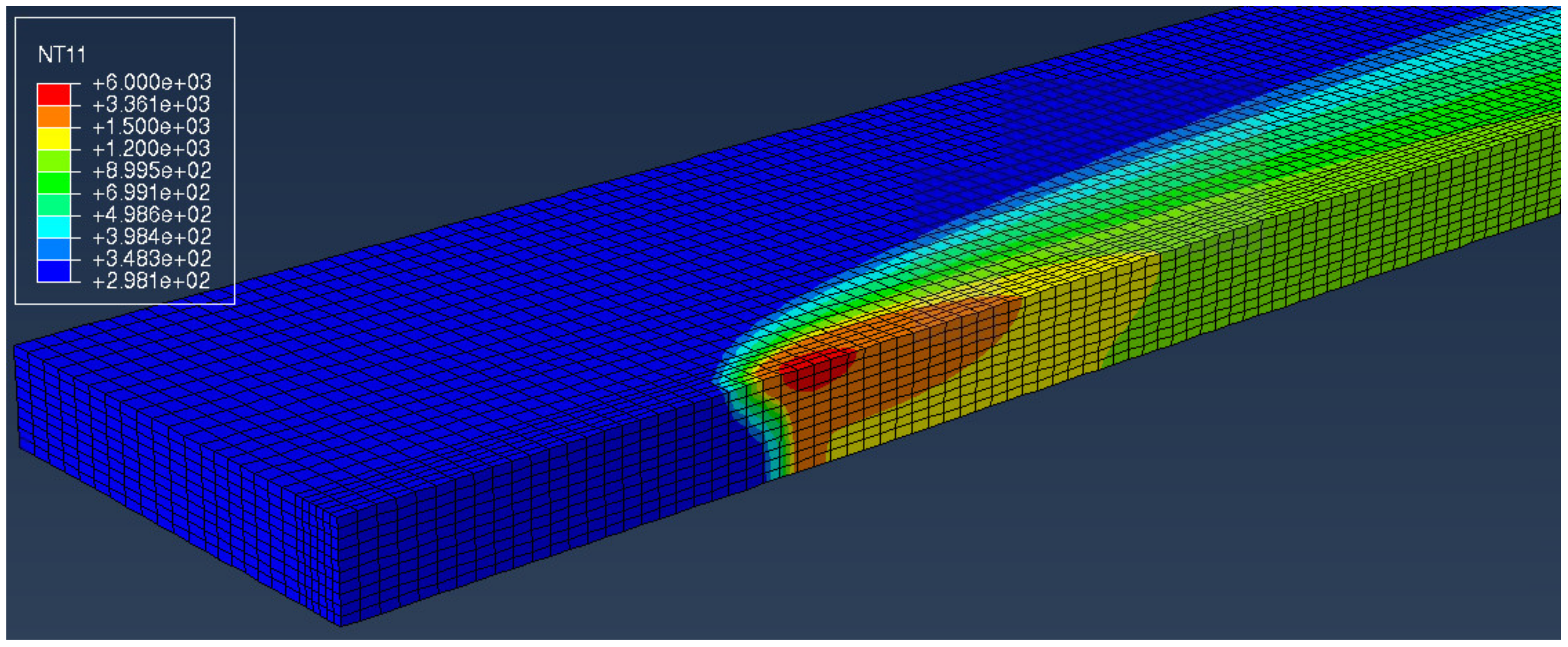
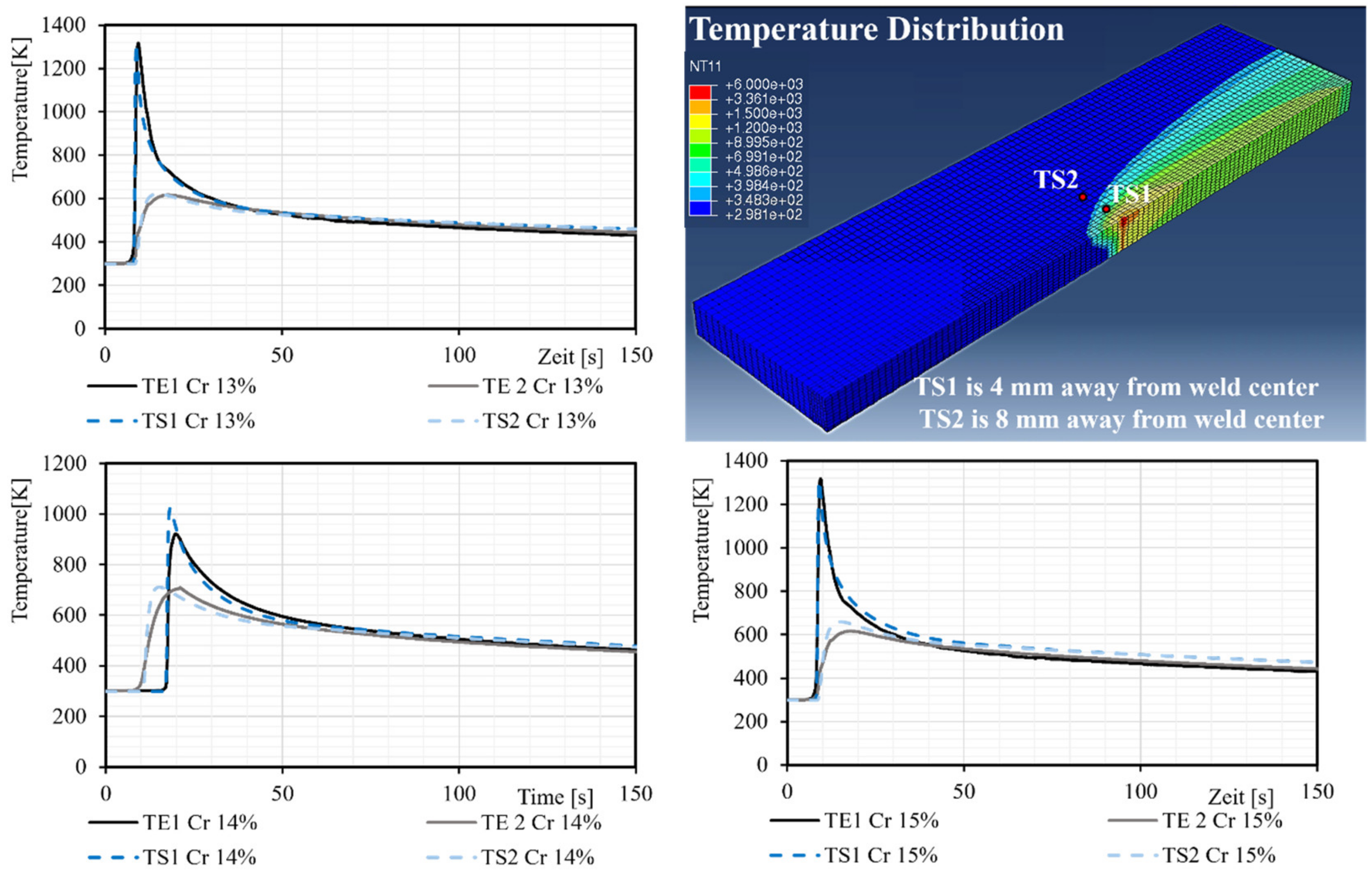
The transient thermal mode (TTM) is a replica of the physical model that was computed using a commercial analysis software—Abaqus 2023. Since the weld was performed in the centre of the specimen in the longitudinal direction, only half of the specimen needs to be simulated due to symmetry. The simulation model was computed by considering the welding parameters, the geometry, the thermal boundary conditions (BC) (convection and radiation) and the temperature-dependent thermal material properties. The material properties for the base plate and weld seam were calculated using Jmat Pro version 13 [29] on the basis of the chemical compositions (Table 1 for the base plate and Table 3 for the weld seam). The thermal BC, convection and radiation were integrated into the thermal simulation with the Abaqus subroutine, SFILM. To minimise computational time, a symmetric finite element method (FEM) model has been implemented, incorporating a plate with dimensions of 100 × 25 × 5 mm, and variable mesh densities were implemented. The author implemented the equivalent heat source model based on their previous work Figure 4 [11], which utilised an eight-node brick element (DC3D8) with a total of 28,886 nodes and 25,000 elements. The implementation of the equivalent heat source was achieved by using an Abaqus DFLUX user subroutine [30]. The TTM is presented in Figure 5.
In this study, a combination of a spherical and a conical heat source model is used to describe a transient heat source model, as in Figure 4 [28,31], where the sphere is used to have a broader weld width and the conical is used to obtain the heat input into the depth of the workpiece.
Q S p e r i c a l = 1 Ψ 6 3 Q R g 3 π π E n e r g y   i n p u t       e x p 3 x 2 R g 2 + y 2 R g 2 + z v t 2 R g 2
Equation (8) describes a Goldak heat source with geometric variables defined to be equal in size, thus representing a sphere with the radius Rg. This serves to simplify the equation and to reduce the variables in the numerical model. The beam power is described by the parameter Q, whereby   Q = P   k e f f ; defined by the laser power and the efficiency coefficient keff. The parameter Ψ describes the portion of the conical heat source and is ≤1. This means, for example, with a Ψ = 0.7, the conical part is effective at 70% and the spherical part at 30%. The movement of the heat source is described by the expression u = x v t . Here, t is the welding time and v is the welding speed.
Q C o n i c a l = 3 Ψ Q π H R 0 2 E n e r g y   i n p u t exp 3 x 2 R 0 2 + z v t 2 R 0 2 1 + 0.01 H y H I n c l i n a t i o n   o f   f l a n k s s t e p H y 1 m m S t e p = 0               i f   H y < 0.0 1               i f   H y > 0.0 0.5         i f   H y = 0.0
Equation (9) is used for the conical heat source. The geometrical contour of the cone is described by the radius R0 and the cone height H. In addition, a term is provided in which the inclination of the cone flanks is described. The energy density distribution in the direction of the weld depth is regulated by the dimensionless step function. The step function is a simulation specification so that the heat input in the y-direction never exceeds the cone height H. If y > H, the step function is set as 0. If y < H, the step function is set as 1. If y = H, the function is set to 0.5.
To represent the total heat source, the conical and spherical heat sources are added up, as in Equation (10) and then the thermal model is computed.
Q L B = Q S p h e r i c a l + Q C o n i c a l
(b)
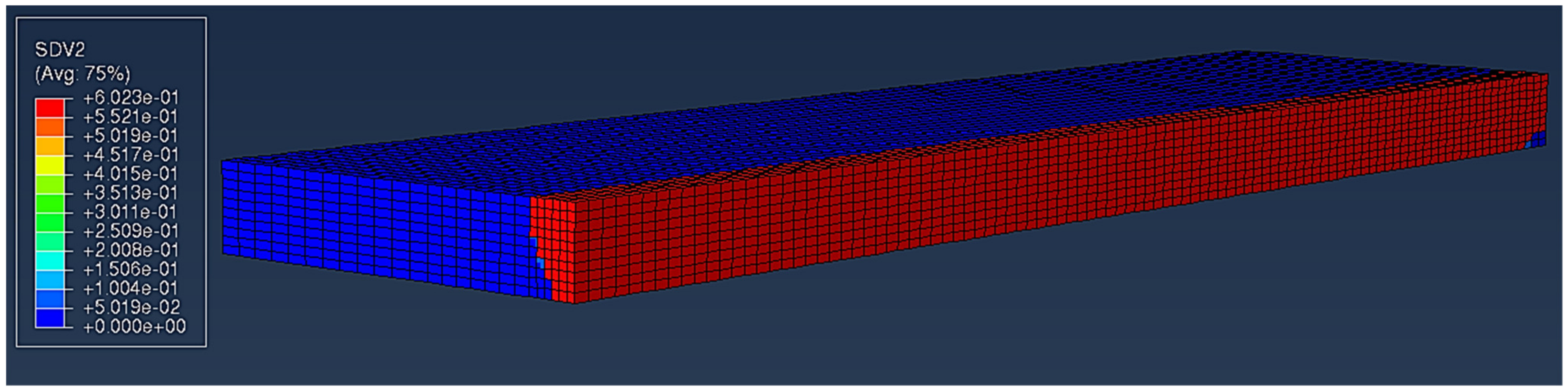
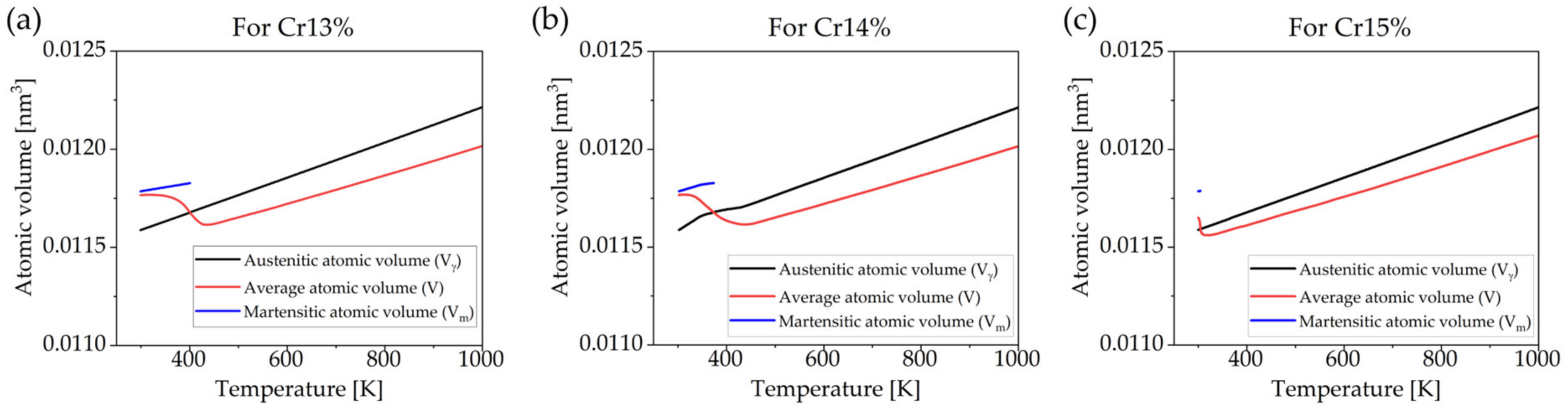
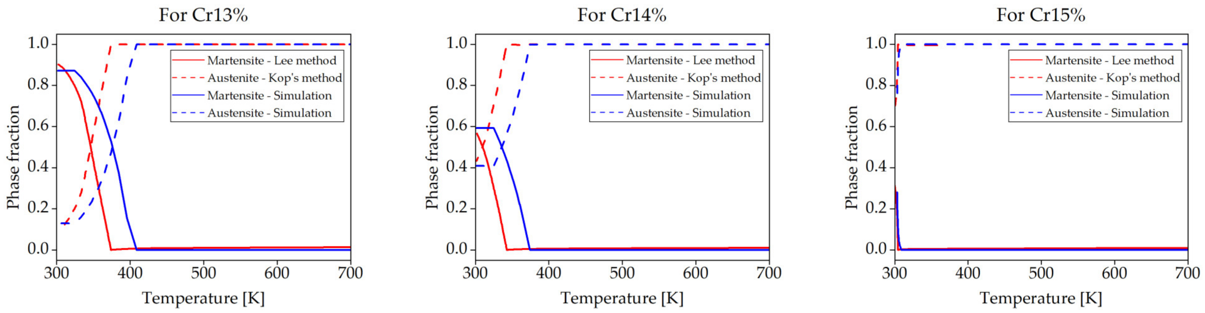
The phase transformation model (PTM) is calculated using the temperature data obtained from the temperature transformation model (TTM), as in Figure 6. Since the main focus of this work is on the cooling cycle, the phase during the heating cycle was considered to be 1 and only in the cooling cycle, the kinematics of austenite to martensite and the retained austenite were calculated using the Koistinen–Marburger numerical Equation (12) [32] and Johnson–Mehl–Avrami numerical Equation (11) [33]. The Abaqus subroutine used for PTM is UEXPAN with solution-dependent variables (SDV).
V γ = V γ 1 exp b γ T n γ
where-,
n γ = ln ln 1 V γ s / ln 1 V γ s f / ln T γ s / T γ f , b γ = n γ 1 V γ f / T γ s
V γ s / V γ f —starting and end volume fraction; V γ —rest austenite volume fraction
T γ s / T γ f —starting and end transformation temperature.
The material constant b was initially assigned a value of 0.011 [34]. The simulation model was then compared with the dilatometer data and the value of the material constant was adjusted to the experimental volume fraction values.
V m = V γ 1 exp b ( M s T
where-,
V m —martensite volume fraction; b—material constant; T—current temperature.

4. Results and Discussion

The dilatometer study carried out on the stainless steel test samples (1.4301 + G3Si1) subjected to laser beam welding showed clear phase transitions indicating the presence of the LTT effect. The observed transitions showed sudden changes in the dimensional response of the material as a function of temperature. Figure 7 represents the volume fractions determined for each composition by analysing the dilatation curves obtained by the dilatometer during the cooling cycle using the lever rule.
The lever rule [21] is a graphical technique used to estimate the volume fractions of the different phases in a material, based on the material’s chemical composition and temperature. This approach is particularly suitable for systems that exhibit equilibrium between two phases. The observed dilatation curves indicate that only austenite and martensite phases are present. Therefore, this method can be used as one of the approaches to determine the proportion of volume fractions. From Figure 7a for Cr 13% the martensite formation begins at M s _Cr13% = 444.2 K and the martensite ends at M f _Cr13% = 340 K. This leads to a complete transformation and a higher change in length, which in turn gives rise to a martensitic volume fraction of V m = 0.95 ,     w hereas Figure 7b,c shows that the martensitic start temperature for Cr14% and Cr15% was found to be M s _Cr14% = 364.7 K and M s _Cr15% = 308.8 K, and the end temperature was much lower than room temperature. This resulted in a reduction in transformation as the change in length was much smaller when compared to Cr13% and, for this reason, the samples were not completely transformed when they reached room temperature. Therefore, the martensitic volume fractions were relatively lower than each other ( C r 14 % V m = 0.75 ,   C r 15 % V m = 0.28 ). From these results, it can be concluded that the LTT effect changes the formation of martensite at reduced temperature and the martensite formation further decreases with increasing Cr-Ni content.
The volume fractions and the atomic volume were empirically calculated using KOP’s and Lee’s method [22,23] by considering the lattice parameter and thermal expansion coefficient Figure 7 and Figure 8.
Figure 8a–c show the austenitic and martensitic volume fractions for Cr 13%, Cr 14% and Cr 15%, while Figure 9a–c represent the austenitic, martensitic and average atomic volume for Cr 13%, Cr 14% and Cr 15%. In the case of Cr 13%, as in Figure 9a, the martensitic atomic volume is much higher, whereas, in Figure 9b,c, the atomic volume formation is very low. This gives a clear indication of the reduction of martensite with increasing Cr Ni composition. The empirical calculations were more reliable than the graphical method (the lever rule) because the graphical method does not consider the kinematics of transformation as it is only based on the equilibrium principle. Table 4 below provides information about the volume fractions and the martensite start temperature, which were calculated empirically.
The initial step in calculating the FEM phase transformation model is the computation of the Transient Temperature Model (TTM). The TTM for each Cr-Ni composition was computed by considering the thermal properties for each case and the equivalent heat source was used from a previous work [11] and validated using the temperature that was experimentally measured using K-type thermocouples Figure 10. The position for temperature measuring (that is, 4 and 8 mm away from the centre of the weld seam) for both simulation and experimental were kept the same. From the plotted graphs for each case, the temperature curves have a very good agreement (approximately 90% and above) in both the heating and cooling cycles.
The thermal history from the TTM for different Cr-Ni compositions is used to compute the phase transformation during welding. In all cases, only the cooling cycle has been discussed, as the resulting transformation will have more influence on distortion and residual stresses. The computed phase transformation has been calibrated in order to match the experimental volume fractions. The below graph is the calibrated FEM phase transformation model compared with the experimental values. Both empirically calculated and simulated volume fractions had a good agreement (above 90%) Figure 11.

Summary and Outlook

This research focused on the phase transformation kinetics in LTT welds with altered chemical composition using numerical simulations, with both empirical and graphical approaches. The change in the chemical composition of chromium and nickel was achieved by varying the weld geometry and welding parameters in the weld. The martensite formation dynamics for different chemical compositions were analysed for high-alloyed base material with low-alloyed filler wire at variations of the chromium content of 13%, 14% and 15%. The martensite start temperature (Ms) was determined to be 400.86 K, 373.8 K and 304.3 K, respectively. A dilatometry experiment was performed to calculate the martensitic phase transformation temperature and the corresponding length change for all compositions. The results show that the Ms temperature decreases with increasing chromium content, which guarantees the LTT effect. The martensitic phase transformation is accompanied by a volume expansion so that the calculation of the volume fraction using an empirical approach allows an accurate calculation of the volume fraction compared to the graphical method. Thus, instead of converting the dilatometry data directly into the volume fraction, calculating the volume fraction dependent on the lattice parameters resulted in better accuracy. The volume fraction simulation model was calibrated against the experimental data to obtain an accurate prediction and showed good agreement (above 90% for empirical and simulated values) with the experimental values. By knowing these volumes, the corresponding strains can be calculated to predict the reduced deformation with the LTT effect. The observed phase transformations and their dependence on the laser beam parameters provide valuable insights into the behaviour of stainless steel with the LTT effect during laser beam welding. The increase in volume due to the formation of the martensitic phase in the weld seam as a result of the LTT effect leads to compressive stresses in the weld seam. Therefore, the prediction of volume fractions using a simulation method with the LTT effect plays a decisive role in understanding and predicting the mechanical behaviour (deformation and residual stresses) after welding.

Author Contributions

K.R.K.M.: Writing—review & editing, Writing—original draft preparation, Visualization, Methodology, Investigation, Formal analysis, Data curation, Conceptualization, validation. F.A.: Investigation. U.R.: Project administration, funding acquisition. S.O.: Project administration, funding acquisition. D.M.: Investigation. All authors have read and agreed to the published version of the manuscript.

Funding

This research was funded by the Deutsche Forschungsgemeinschaft e.V. (DFG, German Research Foundation). The sponsorship and support are gratefully acknowledged.

Data Availability Statement

The research data has been uploaded in the link below and will be made available on request: http://hdl.handle.net/21.11102/efea1a97-ac6f-411b-95ee-78c4a321df2a (accessed on 15 February 2024).

Acknowledgments

The presented investigations were carried out at RWTH Aachen University Welding and Joining Institute ISF within the framework of the Collaborative Research Centre SFB1120-236616214 “Bauteilpräzision durch Beherrschung von Schmelze und Erstarrung in Produktionsprozessen” and simulations were performed with computing resources granted by RWTH Aachen University under project rwth1256.

Conflicts of Interest

Authors have no conflict of interest to declare.

References

  1. Lebedev, A.A.; Kosarchuk, V.V. Influence of phase transformations on the mechanical properties of austenitic stainless steels. Int. J. Plast. 2000, 16, 749–767. [Google Scholar] [CrossRef]
  2. Jiang, W.; Chen, W.; Woo, W.; Tu, S.-T.; Zhang, X.-C.; Em, V. Effects of low-temperature transformation and transformation-induced plasticity on weld residual stresses: Numerical study and neutron diffraction measurement. Mater. Des. 2018, 147, 65–79. [Google Scholar] [CrossRef]
  3. Francis, J.A.; Stone, H.J.; Kundu, S.; Bhadeshia, H.K.D.H.; Rogge, R.B.; Withers, P.J.; Karlsson, L. The Effects of Filler Metal Transformation Temperature on Residual Stresses in a High Strength Steel Weld. J. Press. Vessel Technol. 2009, 131, 041401. [Google Scholar] [CrossRef]
  4. Liu, T.; Liang, L.; Raabe, D.; Dai, L. The martensitic transition pathway in steel. J. Mater. Sci. Technol. 2023, 134, 244–253. [Google Scholar] [CrossRef]
  5. Moyer, J.M.; Ansell, G.S. The Volume Expansion Accompanying the Martensite Transformation in Iron-Carbon Alloys. Metall. Trans. A 1975, 6, 1785–1791. [Google Scholar] [CrossRef]
  6. Akyel, F.; Gamerdinger, M.; Olschok, S.; Reisgen, U.; Schwedt, A.; Mayer, J. Adjustment of chemical composition with dissimilar filler wire in 1.4301 austenitic stainless steel to influence residual stress in laser beam welds. J. Adv. Join. Process. 2022, 5, 100081. [Google Scholar] [CrossRef]
  7. Kromm, A.; Dixneit, J.; Kannengiesser, T. Residual stress engineering by low transformation temperature alloys—State of the art and recent developments. Weld World 2014, 58, 729–741. [Google Scholar] [CrossRef]
  8. Wohlfahrt, H. Die Bedeutung der Austenitumwandlung für eigenspannungs entstehung beim Schweißen. HTM J. Heat Treat. Mater. 1986, 4, 248–257. [Google Scholar] [CrossRef]
  9. Ohta, A.; Maeda, Y.; Nguyen, T.N.; Suzuki, N. Fatigue Strength Improvement of Box Section Member by Using Low Transformation Temperature Welding Material. Q. J. Jpn. Weld. Soc. 2000, 18, 628–633. [Google Scholar] [CrossRef]
  10. Kromm, A.; Kannengiesser, T.; Gibmeier, J.; Genzel, C.; Van Der Mee, V. Determination of residual stresses in low transformation temperature (LTT-) weld metals using X-ray and high energy synchrotron radiation. Weld. World 2009, 53, 3–16. [Google Scholar] [CrossRef]
  11. Akyel, F.; Reisgen, U.; Olschok, S.; Murthy, K. Simulation of Phase Transformation and Residual Stress of Low Alloy Steel in Laser Beam Welding. In Enhanced Material, Parts Optimization and Process Intensification; Reisgen, U., Drummer, D., Marschall, H., Eds.; Springer International Publishing: Cham, Switzerland, 2021; pp. 3–13. [Google Scholar]
  12. Altenkirch, J.; Gibmeier, J.; Kromm, A.; Kannengiesser, T.; Nitschke-Pagel, T.; Hofmann, M. In situ study of structural integrity of low transformation temperature (LTT)-welds. Mater. Sci. Eng. A 2011, 528, 5566–5575. [Google Scholar] [CrossRef]
  13. Krishna Murthy, K.R.; Akyel, F.; Reisgen, U.; Olschok, S. Simulation of transient heat transfer and phase transformation in laser beam welding for low alloy steel and studying its influences on the welding residual stresses. J. Adv. Join. Process. 2022, 5, 100080. [Google Scholar] [CrossRef]
  14. Gottstein, G. Physical Foundations of Materials Science; Springer: Berlin/Heidelberg, Germany, 2004. [Google Scholar]
  15. Hung, T.-S.; Chen, T.-C.; Chen, H.-Y.; Tsay, L.-W. The effects of Cr and Ni equivalents on the microstructure and corrosion resistance of austenitic stainless steels fabricated by laser powder bed fusion. J. Manuf. Process. 2023, 90, 69–79. [Google Scholar] [CrossRef]
  16. Feng, Z.-Y.; Di, X.-J.; Wu, S.-P.; Zhang, Z.; Liu, X.-Q.; Wang, D.-P. Comparison of two types of low-transformation-temperature weld metals based on solidification mode. Sci. Technol. Weld. Join. 2018, 23, 241–248. [Google Scholar] [CrossRef]
  17. Dixneit, J.; Vollert, F.; Kromm, A.; Gibmeier, J.; Hannemann, A.; Fischer, T.; Kannengiesser, T. In situ analysis of the strain evolution during welding using low transformation temperature filler materials. Sci. Technol. Weld. Join. 2019, 24, 243–255. [Google Scholar] [CrossRef]
  18. Feng, Z.; Ma, N.; Hiraoka, K.; Komizo, Y.; Kano, S.; Nagami, M. Development of 16Cr8Ni low transformation temperature welding material for optimal characteristics under various dilutions due to all repair welding positions. Sci. Technol. Weld. Join. 2023, 28, 305–313. [Google Scholar] [CrossRef]
  19. Hosseini, S.A.; Gheisari, K.; Moshayedi, H.; Ahmadi, M.R.; Warchomicka, F.; Enzinger, N. Assessment of the chemical composition of LTT fillers on residual stresses, microstructure, and mechanical properties of 410 AISI welded joints. Weld. World 2021, 65, 807–823. [Google Scholar] [CrossRef]
  20. Kang, J.-Y.; Park, S.-J.; Suh, D.-W.; Han, H.N. Estimation of phase fraction in dual phase steel using microscopic characterizations and dilatometric analysis. Mater. Charact. 2013, 84, 205–215. [Google Scholar] [CrossRef]
  21. Gómez, M.; Medina, S.F.; Caruana, G. Modelling of Phase Transformation Kinetics by Correction of Dilatometry Results for a Ferritic Nb-microalloyed Steel. ISIJ Int. 2003, 43, 1228–1237. [Google Scholar] [CrossRef]
  22. Kop, T.A.; Sietsma, J.; van der Zwaag, S. Dilatometric analysis of phase transformations in hypo-eutectoid steels. J. Mater. Sci. 2001, 36, 519–526. [Google Scholar] [CrossRef]
  23. Lusk, M.T.; Wang, W.; Sun, X.; Lee, Y.K. On the role of kinematics in constructing predictive models of austenite decomposition. In Austenite Formation and Decomposition; The Minerals, Metals & Materials Society: Pittsburgh, PA, USA, 2003. [Google Scholar]
  24. Choi, S. Model for estimation of transformation kinetics from the dilatation data during a cooling of hypoeutectoid steels. Mater. Sci. Eng. A 2003, 363, 72–80. [Google Scholar] [CrossRef]
  25. Ravi, K.; Murthy, K.; Fatma, A.; Simon, O.; Uwe, R. (Eds.) LTT Effect Simulation by Varying the Cr-Ni Compositions in the Weld Zone during Laser Beam Welding for High Alloy Steel and Studying Its Influence on Ms Temperature and Residual Stresses. In Proceedings of the Lasers in Manufacturing Conference 2023, Munich, Germany, 26–29 June 2023. [Google Scholar]
  26. ISO 13919-1:2019; Electron and Laser-Beam Welded Joints Requirements and Recommendations on Quality Levels for Imperfections Part 1: Steel, Nickel, Titanium and Their Alloys, 2nd ed. International Standard Published, 2019. Available online: https://www.iso.org/standard/75514.html (accessed on 15 February 2024).
  27. A01 Committee. Practice for Quantitative Measurement and Reporting of Hypoeutectoid Carbon and Low-Alloy Steel Phase Transformations; ASTM International: West Conshohocken, PA, USA, 2018. [Google Scholar]
  28. Goldak, J.A.; Akhlaghi, M. Computational Welding Mechanics; Springer: New York, NY, USA, 2005. [Google Scholar]
  29. Saunders, N.; Guo, U.K.Z.; Li, X.; Miodownik, A.P.; Schillé, J.P. Using JMatPro to model materials properties and behavior. Jom 2003, 55, 60–65. [Google Scholar] [CrossRef]
  30. Abaqus User Subroutines Reference Guide; Version 6.14; Dassault Systèmes: Vélizy-Villacoublay, France, 2014.
  31. Goldak, J.; Chakravarti, A.; Bibby, M. A new finite element model for welding heat sources. Metall. Trans. B 1984, 15, 299–305. [Google Scholar] [CrossRef]
  32. Deng, D. FEM prediction of welding residual stress and distortion in carbon steel considering phase transformation effects. Mater. Des. 2009, 30, 359–366. [Google Scholar] [CrossRef]
  33. Winczek, J.; Skrzypczak, T. Thermomechanical States in Arc Weld Surfaced Steel Elements. Arch. Metall. Mater. 2016, 61, 1623–1634. [Google Scholar] [CrossRef]
  34. Dean, D.; Yu, L.; Hisashi, S.; Masakazu, S.; Hidekazu, M. Numerical Simulation of Residual Stress and Deformation Considering Phase Transformation Effects(Mechanics, Strength & Structural Design). Trans. JWRI 2003, 32, 325–333. [Google Scholar]
Figure 1. (a) Welding setup at Welding and Joining Institute, RWTH Aachen; (b) thermocouple setup for temperature measurement; (c) weld cross section for Cr 13%; (d) weld cross section for Cr 14%; (e) weld cross section for Cr 15% [25].
Jmmp 08 00050 g001
Figure 2. (a) Dilatometer sample preparation and (b) dilation curves for Cr 13%, Cr14% and Cr15%.
Jmmp 08 00050 g002
Figure 3. Extrapolated dilation curves during cooling for Cr 13%, Cr 14% and Cr 15%.
Jmmp 08 00050 g003
Figure 4. Combined spherical and conical heat source model.
Jmmp 08 00050 g004
Figure 5. Transient thermal model with temperature distribution along the plate.
Jmmp 08 00050 g005
Figure 6. Phase transformation model (martensite).
Jmmp 08 00050 g006
Figure 7. Volume fraction for Cr 13%, Cr14% and Cr15% using lever rule.
Jmmp 08 00050 g007
Figure 8. Volume fraction for Cr 13%, Cr14% and Cr15% using lattice parameter, thermal expansion and carbon content.
Jmmp 08 00050 g008
Figure 9. Austenitic, martensitic and average atomic volume for Cr 13%, Cr14% and Cr15% using lattice parameter, thermal expansion and carbon content.
Jmmp 08 00050 g009
Figure 10. Experimental (TE) and simulation (TS) temperature distribution comparison.
Jmmp 08 00050 g010
Figure 11. Volume fractions comparison of simulation, empirical and graphical, for Cr13%, Cr14% and Cr15%.
Jmmp 08 00050 g011
Table 1. Base (1.4301) and filler (G3Si1) material chemical compositions [25].
MaterialFe
[wt%]
C
[wt%]
Si
[wt%]
Mn
[wt%]
Cr
[wt%]
Ni
[wt%]
Mo
[wt%]
1.430170.70.020.421.6818.28.240.036
G3Si197.30.070.861.440.0450.0190.008
Table 2. Welding parameter, oscillation parameter and weld seam geometry [25].
Oscillation ParameterSeam PreparationJmmp 08 00050 i001
NamePower P [kW]Weld Speed Vw [m/min]Feed Speed Vf [m/min]Frequency F [Hz]Amplitude [%]Figure [-]Width W [mm]Depth D [mm]
LTT-Cr-1360.86.91503Sine1.41.4
LTT-Cr-145.80.83.41505Sine1.61.0
LTT-Cr-155.80.83.41505Sine1.41.0
Table 3. Chemical compositions in the weld seam for different Cr-Ni.
Material in Weld SeamFe
[wt%]
Si
[wt%]
Mn
[wt%]
Cr
[wt%]
Ni
[wt%]
LTT-Cr-13%79.6380.4501.32612.9365.647
LTT-Cr-14%77.4210.4551.46314.5756.084
LTT-Cr-15%76.1710.4131.39915.1736.845
Table 4. Volume fractions of austenite, martensite and martensite start temperature for different Cr-Ni.
Cr 13%Cr 14%Cr 15%
V γ 0.0980.4330.686
V M 0.9010.5660.31
M S 400.86 K373.8 K304.2 K
Disclaimer/Publisher’s Note: The statements, opinions and data contained in all publications are solely those of the individual author(s) and contributor(s) and not of MDPI and/or the editor(s). MDPI and/or the editor(s) disclaim responsibility for any injury to people or property resulting from any ideas, methods, instructions or products referred to in the content.

