Article

High-Fidelity 2-Way FSI Simulation of a Wind Turbine Using Fully Structured Multiblock Meshes in OpenFoam for Accurate Aero-Elastic Analysis

1
Department of Mechanical and Aerospace Engineering, Nazarbayev University, Nur-Sultan 010000, Kazakhstan
2
School of Hydraulic Engineering, Dalian University of Technology, Dalian 116024, China
3
School of Mechanical and Aerospace Engineering, Nanyang Technological University, Singapore 639798, Singapore
*
Author to whom correspondence should be addressed.
Fluids 2022, 7(5), 169; https://doi.org/10.3390/fluids7050169
Submission received: 3 February 2022 / Revised: 6 April 2022 / Accepted: 22 April 2022 / Published: 11 May 2022

Abstract

:
With increased interest in renewable energy, the power capacity of wind turbines is constantly increasing, which leads to increased rotor sizes. With ever larger rotor diameters, the complex and non-linear fluid-structure interaction (FSI) effects on wind turbine aerodynamic performances become significant, which can be fully studied using hi-fidelity 2-way FSI simulation. In this study, a two-way FSI model is developed and implemented in Openfoam to investigate the FSI effects on the NREL Phase VI wind turbine. The fully structured multiblock (MB) mesh method is used for the fluid and solid domains to achieve good accuracy. A coupling method based on the ALE is developed to ensure rotation and deformation can happen simultaneously and smoothly. The simulation results show that hi-fidelity CFD (Computational Fluid Dynamics) and CSD (Computational Structural Dynamics) -based 2-way FSI simulation provides high accurate results for wind turbine simulation and multi-disciplinary design optimization (MDO).

Graphical Abstract

1. Introduction

Due to technological development and increase in population, worldwide energy consumption is constantly increasing. In 2005, worldwide electricity consumption was about 50 quadrillion Btu [1]. According to calculations, by 2040 the energy consumption is increased up to 125 quadrillion Btu [1]. Almost all this energy is coming from burning fossil fuel. According to US Energy Information Administration [2], in 2018 only 15% of worldwide energy consumption is coming for renewable energy sources. At the same time, almost 82% of world consumed energy in 2018 was produced by petroleum, coal, or natural gases [2].
As rotor diameters are increasing, the effects of blade deformation on aerodynamic performances become more significant and cannot be neglected in simulations. Because wind turbine aerodynamics includes rotational motion, the angle of attack along the blade varies with span [3]. The deformation of a blade changes the angle of attack, altering the aerodynamic performance of a wind turbine. Commonly, wind turbine blades are constructed with different materials, which creates regions with different elasticity. This deformation or morphing changes the angle of attack for individual regions of the blade, increasing wind turbine performances [4].
Apart from changing aerodynamic behaviour, blade deformation decreases its durability [5]. According to a study conducted by Liu [5] when a blade is rotating toward its bottom position, the blade deformation increases until the deformation suddenly drops when it is passing the tower. This change of deformation causes decrease in blade durability due to fatigue. Moreover, the power output of a wind turbine increases with rotor area, which has square power relation to the blade radius. However, wind turbine weight increases with the blade radius cubed. Thus, increase in wind turbine power leads to dramatic increase in weight and, therefore, in blade deformation [4]. Thus, during wind turbine design, both structural deformation and aerodynamic properties should be simulated simultaneously, which will also form the basis for multi-disciplinary design optimisation (MDO).
To simulate the interaction between a blade and airflow, CFD simulations should be paired with Computational Solid Dynamics (CSD) simulations. This combined CFD and CSD simulation is called Fluid Structure Interaction (FSI) simulation. The main advantage of FSI simulation is that the effects of aerodynamic loadings on structures and structural deformation on the flow field can be studied simultaneously. For some cases, FSI simulation is mandatory to use. For example, in Manenti’s [6] work, FSI simulation was used to simulate the effect of waves on floating offshore wind turbines. Several other FSI studies have also been done on the wind turbine [7,8,9,10,11]. Another example of FSI simulation implementation is the simulation of a parachute [12].
Another advantage of FSI simulation is increased accuracy. According to Galvani [3], from a wind turbine control perspective, there are three models of wind turbines: low, medium, and high fidelity. The low-fidelity models consist of baseline CFD simulation with the control of pitch angle or rotor speed control. The medium fidelity models cover previously listed models with the consideration of extreme weather and variable/complex wind conditions (using solvers, such as NREL FAST solver [3]). The high-fidelity models include detailed CFD simulation coupled with fluid-structure interaction. Despite this classification being based on wind turbine control systems, it shows that FSI simulations are considered as a high-precision tool for representing a wind turbine model.
Currently, there are commercial programs which support FSI simulations, such as ANSYS, COMSOL, and ADINA. However, researchers prefer open-source programs in their studies [13]. The most popular open-source program is OpenFoam. Due to the open-source nature of these programs, they are highly customisable for different purposes and equipment, which allows them to have better power scaling on HPC clusters in comparison with commercial programs [13].
There are different types of the OpenFoam with multiple versions, which were developed for different purposes. The most recent versions are: OpenFoam.org, OpenFoam.com, and Foam-extend [14]. Among all versions, Foam-extend is the friendliest for source code modifications [13]. Because of this, there are a few modifications for the foam-extend, which include FSI solvers. One of the most popular is Solids4Foam, developed by Philip Cardiff [15]. The other alternatives utilise third-party interfaces, like Precice [16], to connect CFD and CSD simulations.

2. Governing Equations

2.1. Unsteady Reynolds-Averaged Navier-Stokes Flow Model (URANS)

Before starting the simulation, several assumptions need to be made to make above equations easier to solve. Thus, the flow is three-dimensional, unsteady, and incompressible. Fluid flow is expressed using Navier Stokes equations, such as continuity equation and momentum equations [17]:
ρ t + ρ . V = 0
ρ u t = p x + τ x x x + τ x y y + τ x z z + ρ f x
ρ v t = p y + τ y x x + τ y y y + τ y z z + ρ f y
ρ w t = p z + τ z x x + τ z y y + τ z z z + ρ f z
The viscous stresses are defined using following equations:
τ x x = 2 μ f u x 2 3 μ f · V ,   τ x y = τ y x = μ f v x + u y
τ y y = 2 μ f v y 2 3 μ f · V ,   τ x z = τ z x = μ f u z + ω x
τ z z = 2 μ f ω z 2 3 μ f · V ,   τ y z = τ z y = μ f ω y + v z
One of the most popular ways to model turbulence is to use Reynolds averaging on the Navier-Stokes equations. This averaging is presented in Equation (9) [18], where   ϕ represents any time- and space-dependent variable, ϕ ¯ is a mean value component of this variable, and ϕ is a fluctuating component of this variable.
ϕ x , t = ϕ ¯ x , t + ϕ x , t
To calculate the mean value component, the Equation (12) is used:
ϕ ¯ x , t = lim T 1 T t T t ϕ x , t d t
The averaging should be applied to every term of the Navier-Stokes equations from Equation (1) to Equation (7). The unsteady Reynolds-Averaged-Navier-Stokes (URANS) equations for incompressible flows thus results from the above averaging:
· ρ V ¯ = 0
t ρ V ¯ + · ρ V V ¯ = p ¯ + · τ ¯ ρ V V ¯ + f b ¯
The turbulence is calculated using several turbulence models. One of the earliest turbulence models is k ε . This model is good for calculating far field turbulence [18]. To increase accuracy of turbulence prediction near the wall, the k ω model was introduced. This model uses k and ω , which are turbulence kinetic energy and turbulence specific dissipation rate respectively. The k   and ω are calculated using Equations (12) and (13), where I is turbulent intensity, U i n f is free stream velocity, C μ is equal to 0.09, and L is a reference length:
k = 3 2 I U i n f 2
ω = k C μ L
The Navier Stokes equations with k ω model is given below:
ρ ω t + · ρ V ω = · μ e f f , ω ω + S ω
ρ k t + · ρ V k = · μ e f f , k k + S k
where,
S ω = C α 1 ω k P k C β 1 ρ ω 2
S k = P k β ρ k ω
C α 1 = 5 9 ,   C β 1 = 0.075 ,   β = 0.09 (Default model constants by OpenFoam).
There is another popular modification of k ω model, called Shear Stress Transport (SST) which is going to be used for simulation of this model since it is the most accurate and popular model respectively to mesh quality and other parameters. This modification introduces principal shear stress τ x y as:
τ x y = μ t Ω = ρ a 1 k
where turbulent viscosity μ t is calculated using:
μ t = ρ a 1 k M A X a 1 ω , 2 S t F 2
The modified equations for the k ω SST model is thus given below [19]:
D ρ ω D t = · ρ D ω ω + ρ γ G v 2 3 ρ γ ω · u ρ β ω 2 ρ F 1 1 C D k ω + S ω
D ρ k D t = · ρ D k k + ρ G 2 3 ρ k · u ρ β ω k + S k

2.2. Structural Model

The structural simulation, used in this model, does not include temperature effect. Therefore, for this chapter, the simulation would be set to isothermal. The momentum balance state equation has the following form [20]:
2 ρ u t 2 · σ = 0
where u and σ are displacement vector and stress tensor, respectively, while μ s and λ are the material properties. The stress tensor is specified using strain tensor ε :
σ = 2 μ s ε + λ t r ε I
ε = 1 2 u + u T
Combining Equations (23) and (24) will result in following:
· σ = · μ s u + · μ s ( u T + λ I t r u ]
By rearranging terms in Equation (25), the convergence of a simulation is improved [20] due to the modification for the solution algorithm. OpenFoam solves the first term of the Equation (22) implicitly and the second term explicitly [20].
Therefore, by rearranging terms, the explicit and implicit parts become more balanced. The modified version of Equation (22) has the following form:
· σ = · 2 μ s + λ u + · μ s ( u T + λ I t r u μ s + λ u ]
The traction force boundary condition has the following expression (where n is a surface normal to the boundary):
T = σ · n = 2 μ s + λ u + · μ s ( u T + λ I t r u μ s + λ u ] · n
Equations from (22) to (27) describe only elastic deformation. In nature, every material, after reaching some stress level, experience plastic deformation. The modified governing equation with plastic term has the following form [20]:
· { μ s d u + μ s d u T + λ I t r d u 2 μ s d ε p + λ I t r d ε p = 0
where d u and d ε p are incremental displacement vector and incremental plastic strain tensor respectively. Equation (29) undergoes similar modification:
T = σ · n d T = d σ · n = 2 μ s + λ d u + μ s d u T + λ I t r d u μ s + λ d u 2 μ s d ε p + λ I t r d ε p

2.3. Arbitrary Langragian Eulerian (ALE) Method

For FSI simulations, mesh deformation should be calculated after converging fluid and solid solutions. There are three common methods for coupling fluid flow and structural solvers: Eulerian, Arbitrary Lagrangian-Eulerian (ALE), and Chimera or overset methods [17,21]. The ALE is an arbitrary hybrid combination of Eulerian and Lagrangian methods, which are used for fixed and moving meshes, respectively [22]. In order to compensate velocity calculation for dynamic mesh, the mesh velocity V g should be subtracted from fluid velocity in the Navier- Stokes equations. Thus, the governing Equations (10) and (11) will be modified [19] as follows:
· V V g = 0
V t + · V V g V = 1 ρ p + · v e f f V
Taking into account the k ω SST model, the governing equation will have the following formulation:
k t + · V V g k · v v t α k k = 1 ρ P k β ω k
ω t + · V V g ω · v v t α ω ω = ρ C 1 P v t C 2 ω 2 + 2 α ε 1 F 1 ω k · ω
Solid simulations almost always result in movement or deformation. In this case, mesh should be deformed according to results from these simulations. This mesh deformation problem is solved by the following methods: spring analogy, pseudo-solid, and Laplace smoothing.
The first method introduces a spring like connection between vertices. In OpenFoam, the interface between solid and fluid meshes is called moving wall. The first step in calculating mesh deformation using spring analogy method is to identify moving wall nodes. This is done by calculating distance between the node and the wall. After all wall nodes are located and the displacement of these nodes are obtained, the deformation of other nodes is calculated as a function of distance and displacement of a wall node. This method has restrictions because large deformations cause mesh vertices to collide and intersect with each other [23,24]. However, this problem is solved by using torsion springs, non-linear springs, and smoothing procedures [17,25]. The smoothing procedure uses displacement of neighbor nodes to smooth node displacement. Equation (34) describes the smoothing of deformation of a node P:
δ r P = i = 1 N P i δ r i i = 1 N P i
where number N indicated quantity of surrounding edges, P i is the distance between the nodes, connected by edge i and δ r i is the displacement of the node, located at the opposite side of the edge i .
An FSI is a constant simulation with coupled fluid and solid models. The pressure and viscous forces are calculated in fluid simulation and transferred to the solid model. After solid simulation is done, the displacement and velocity information are transferred to the fluid model through the fluid-solid interface. In both fluid and solid simulations, residuals are calculated independently. During simulation in a time step, after transferring the data, the residuals for the coupling equations at the fluid-solid interface between fluid and solid domain are calculated. When these residuals become smaller than the required level, the final mesh is obtained at the end of the time step and time marching can proceed to the next time step.

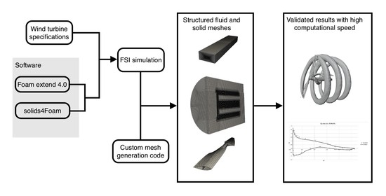
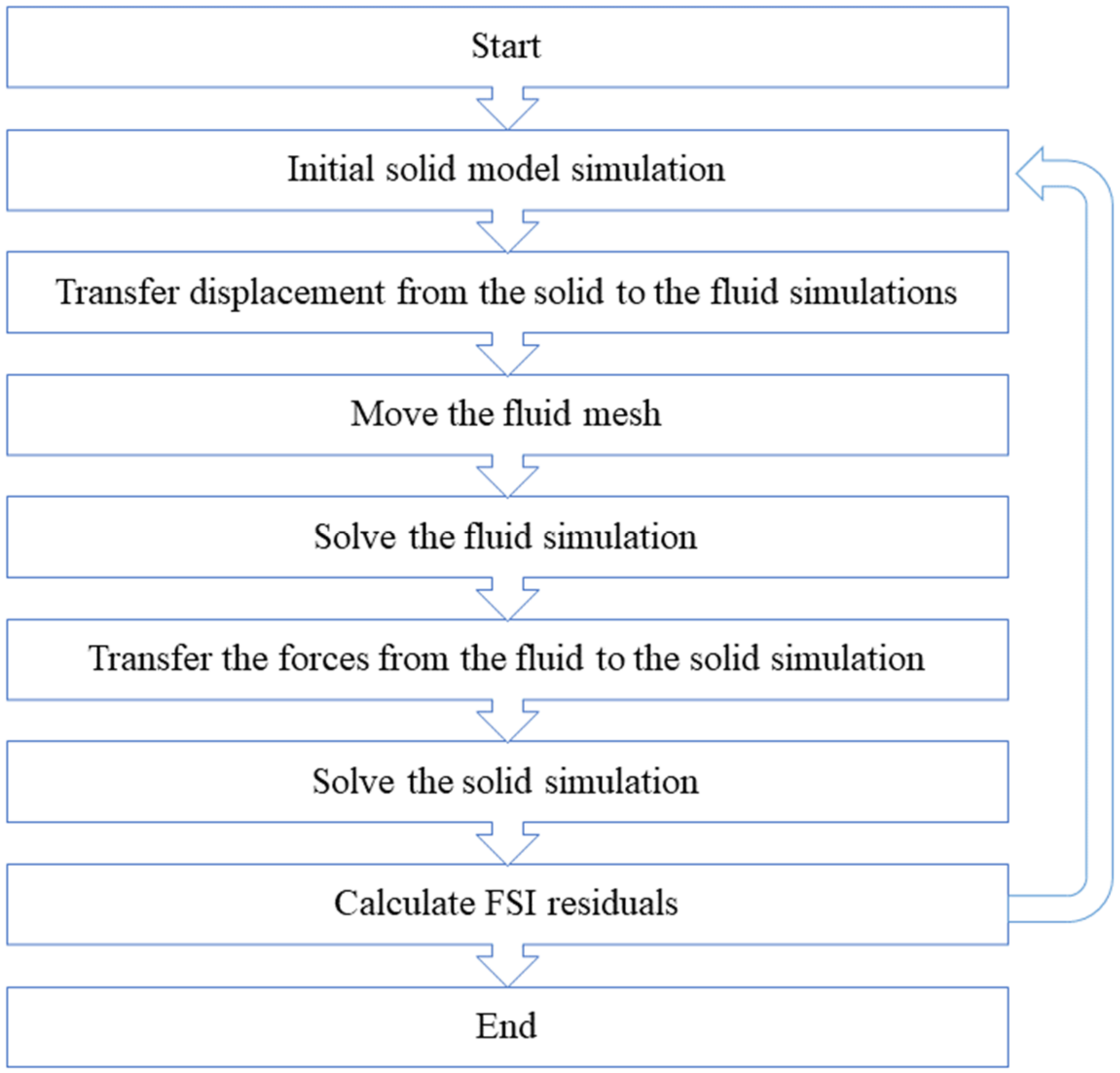
3. OpenFOAM Structure

The main solver is located at solids4Foam/applications/solvers/solids4Foam/at the BitBucket (GitHub. 2022. GitHub - lppferreira/solids4foam. (online) Available at: <https://github.com/lppferreira/solids4foam> (accessed on 2 February 2022). This code controls the whole simulation process by initializing the required classes and calling their methods. The main function of this code is to start the following scripts:
  • Solids4Foam/src/solids4FoamModels/physicsModel/physicsModel.C
  • Solids4Foam/src/solids4FoamModels/fluidModels/fluidModel/fluidModel.C
  • Solids4Foam/src/solids4FoamModels/solidModels/solidModel/solidModel.C
The physics model script collects information about simulation type and simulation parameters. In case of FSI, the physics properties become two-way FSI with Aitken interface coupling with GGI (General Grid Interface) interface interpolation. The solid model and fluid model scripts collect solid and fluid simulation parameters respectively. The scheme of FSI simulation is illustrated in Figure 1.

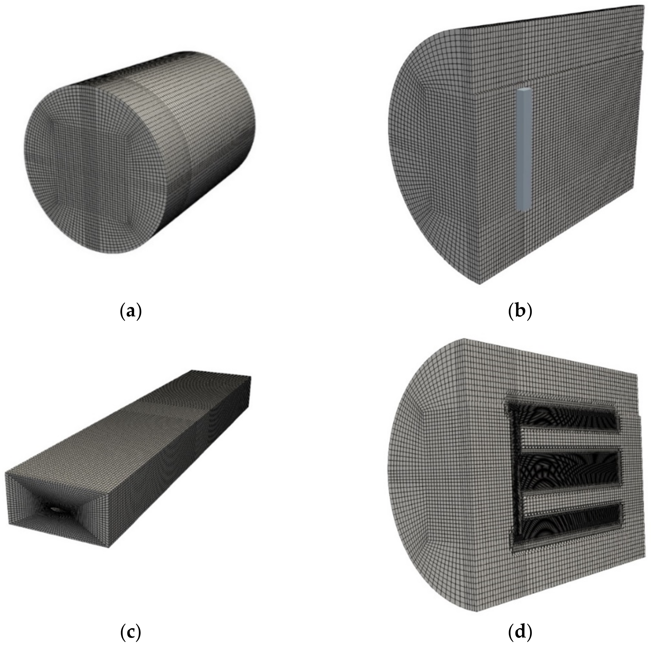
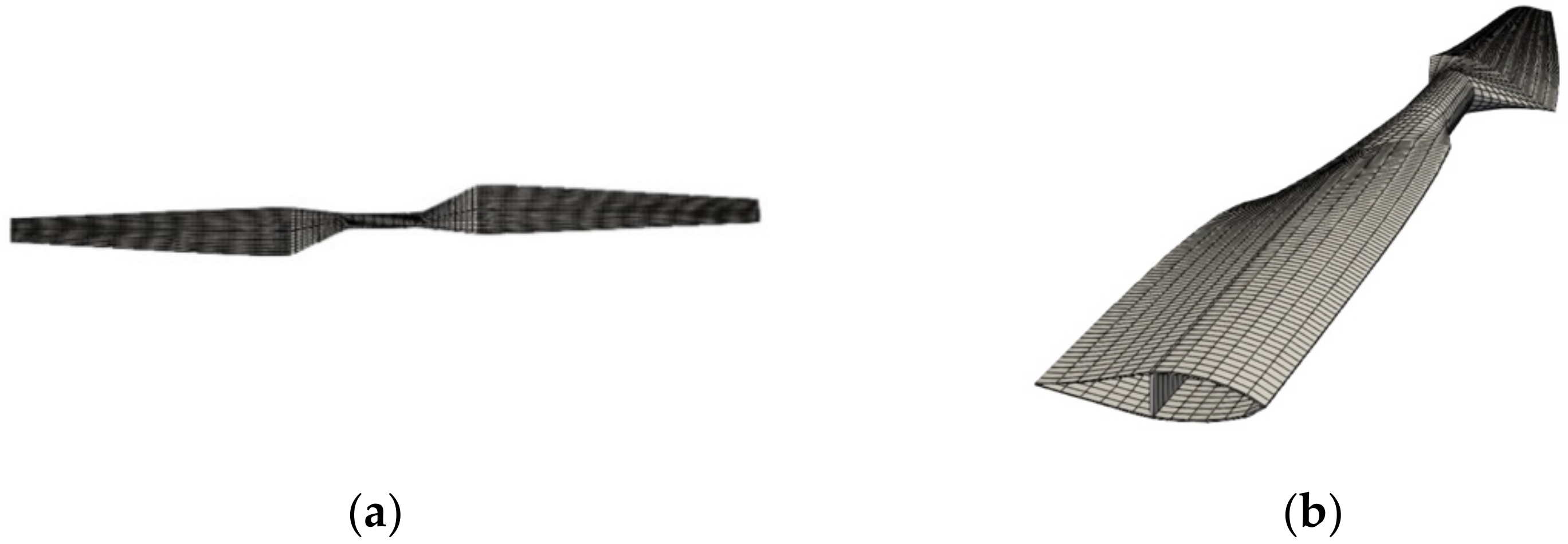
4. Simulation Models and Mesh Generation

In this work, the NREL Phase VI wind turbine would be simulated. Therefore, the airfoil data was imported from the NREL report [26]. The wind speed of 7 m/s and rotational speed of 72 rpm was chosen as in the experimental setup [27].
According to several works [28,29,30], the domain size should be 2D in diameter and 10D in length. It was found that increasing domain length further than 10D has negligible effect on the accuracy of a simulation [31].
Both fluid and solid simulations are using structured mesh for two reasons: (1) to increase computation speed and (2) to have better alignment between fluid and solid interfaces. The first step is to create a fluid domain mesh using BlockMesh. The mesh is as presented in Figure 2a. This mesh fills a cylinder with box-like space in the center, which should contain the refined blade mesh (Figure 2b).
The central part of the fluid mesh was created separately, using a custom Python code (see Appendix). This code extracts coordinates of airfoils from a blade model and prepares a BlockMeshDict file for the BlockMesh for mesh generation. The central mesh created is as represented in Figure 2c.
The next step is to merge blade and domain meshes. This procedure was done using the command mergeMesh. After obtaining combined mesh, required regions were further refined using SnappyHexMesh. The cross-sectional view of the final mesh is as shown in Figure 2d.
Solid blade mesh was created with the same code as fluid mesh. The solid blade has internal structure, which represents the real blade [26] as shown in Figure 3a,b.

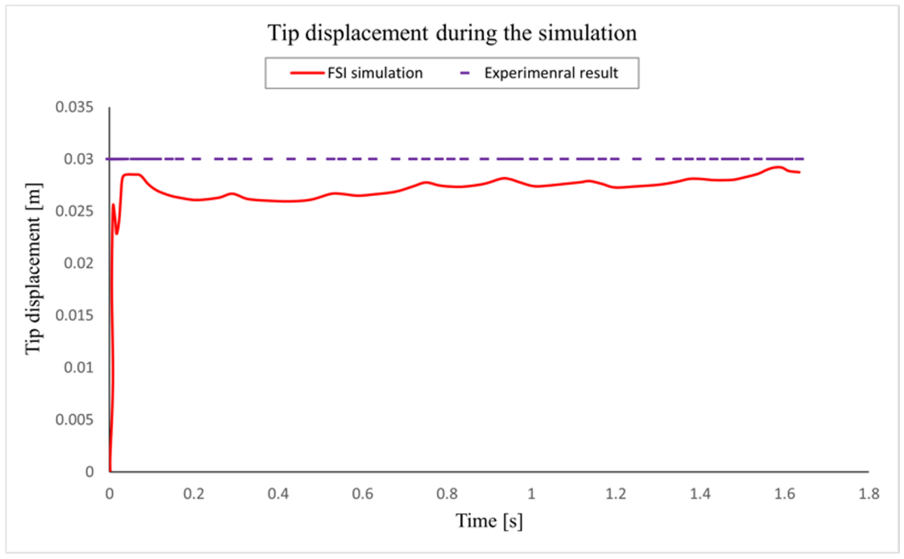
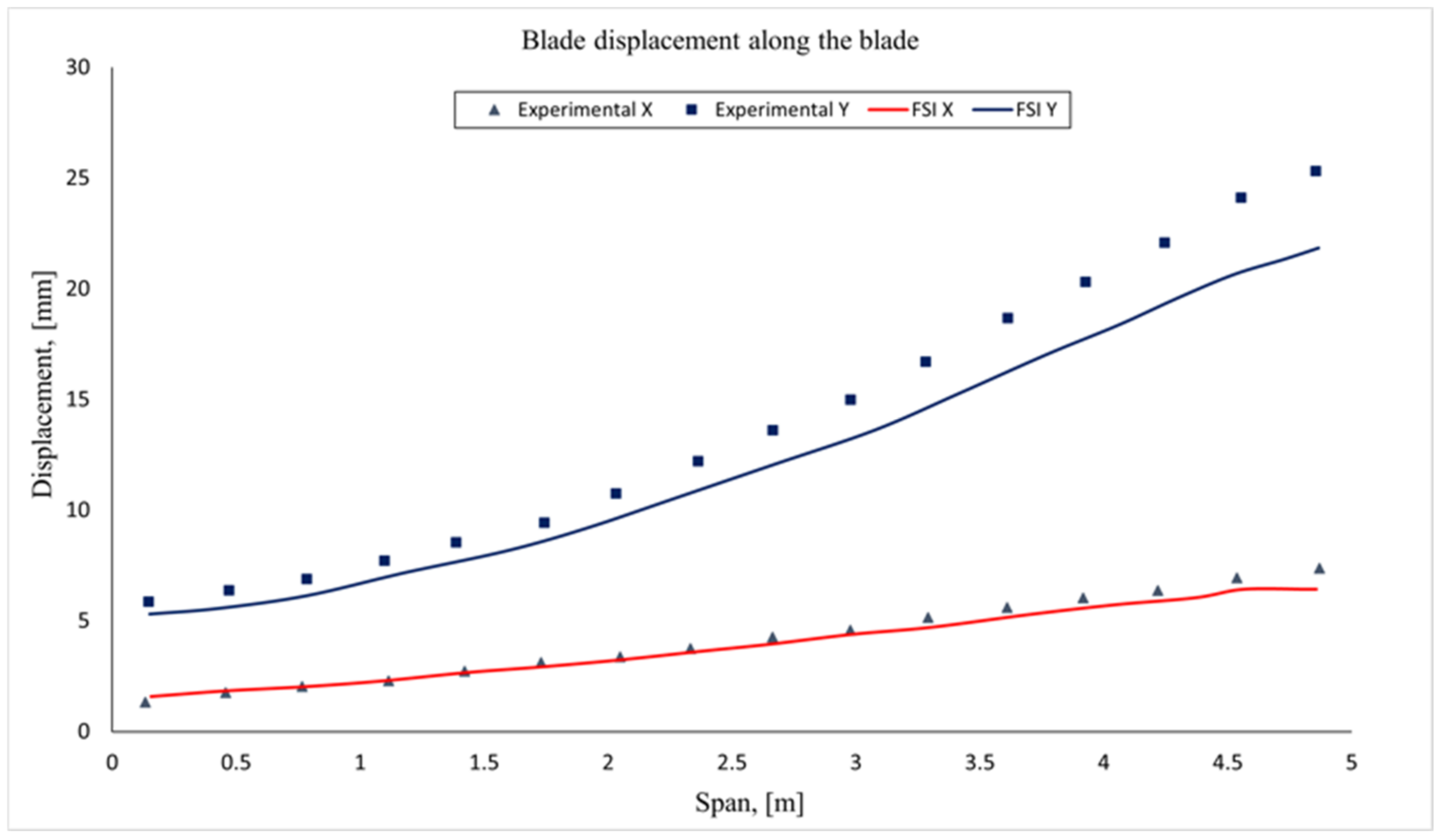
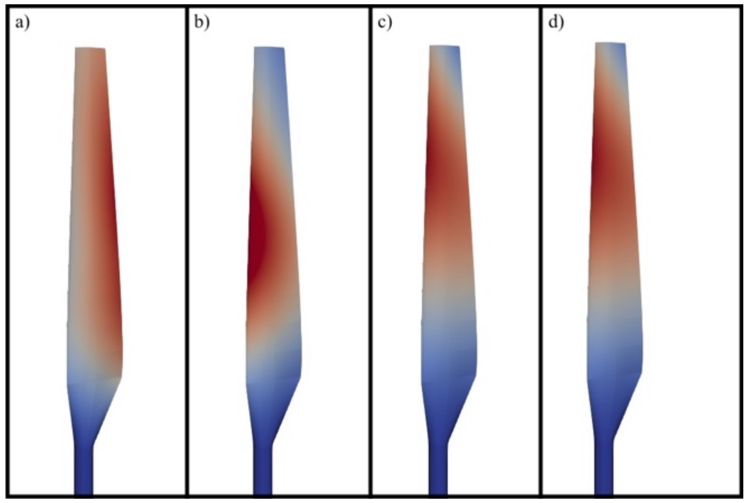
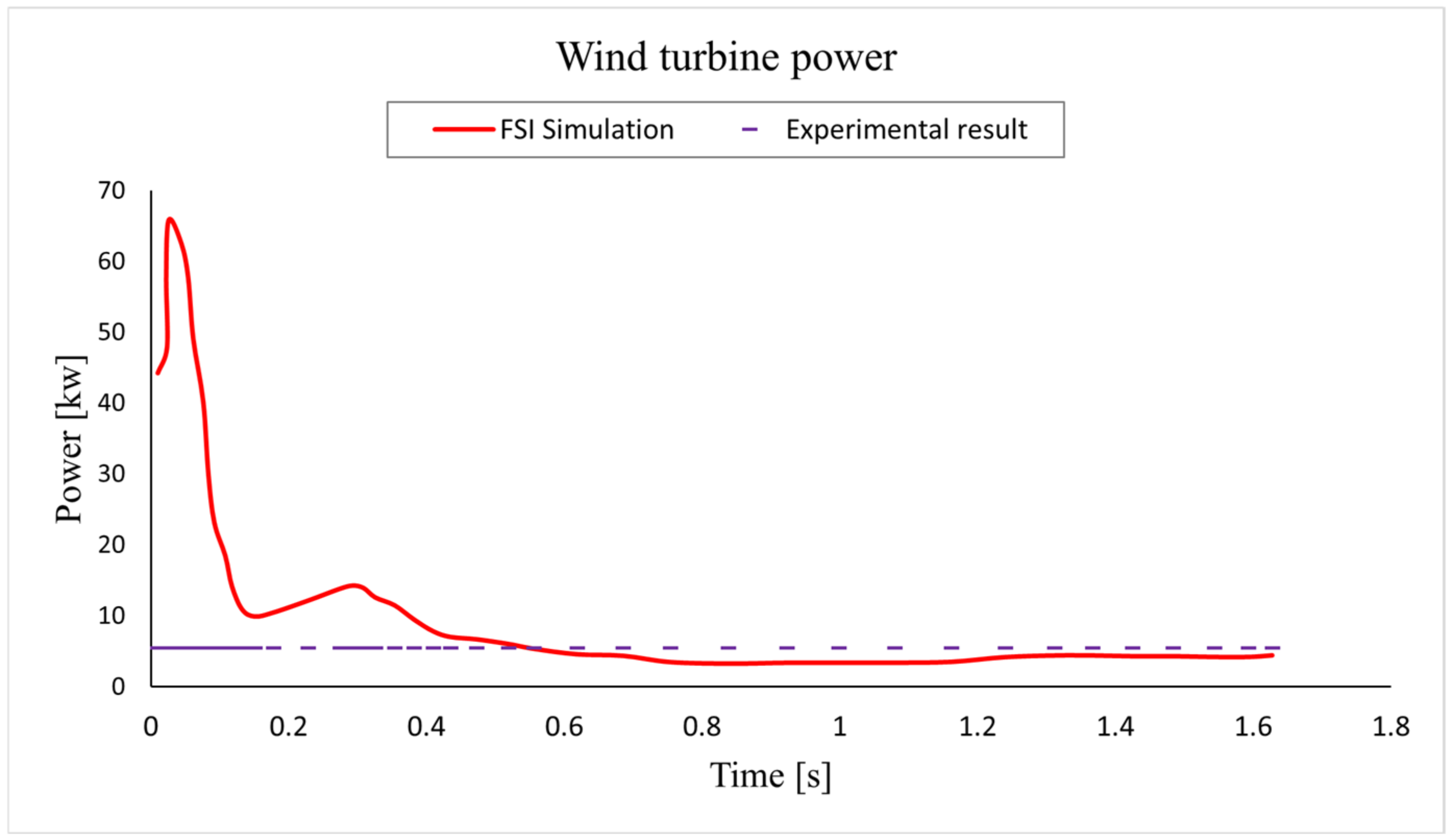
5. Simulation Results and Discussion

A mesh convergence study should be done to prove that simulation results are not dependent on mesh size, which was performed by comparing results for different mesh densities until key parameter percentage variation falls below 1%, which is the percentage difference of power coefficients between previous and present meshes in this study. The results of the mesh convergence study are listed in Table 1. Thus, the mesh with 15,240,561 cells was used for further study.
Figure 4 shows pressure contour results for around the blade for r/R = 46.6%, which are similar to other researchers’ work [27]. The wake vorticities are viewed in Figure 5 as vorticity iso-surfaces, where both blade tip and root vorticities are clearly seen.
One of the most important validation procedures is to compare pressure coefficient over the blade surfaces with experimental measurements. The results are viewed in Figure 6, where it is clearly seen that simulation results are accurate in comparison with experimental values [27].
Table 2 shows the material properties of the solid blade that is used for CSD part of the simulation.
Figure 7 shows the predicted tip displacement. The experimental values show 30 mm in displacement for 7 m/s [32]. According to the figure, the simulation results under predict the deformation values during the whole simulation period. According to Lee [32], all the published studies using various models tend to under predict blade deformation, however, the current FSI method gives more accurate results.
The displacement distribution along the blade over its span can be viewed in Figure 8. These data were calculated as time averaged values over the whole simulation cycle and are compared with the corresponding experimental measurements. The simulation results slightly under predict deformation by comparison, which correlates with other simulation types [32] but with better accuracy.
Figure 9 shows pressure distribution over the blade over whole simulation time. It is clearly seen, that at the beginning of the simulation, most pressure were concentrated at the trailing edge of the blade. As simulation is progressed, the pressure distribution was changed to the leading edge of the blade.
The values of power are as shown in Figure 10, where the solid line represent simulated values and dashed line represent experimental values for 7 m/s. There is a peak in power values at the start of the simulation, which is explained by the FSI simulation methodology. Both fluid and solid simulations use the numerical method, which cannot provide accurate values at the start of the simulation. However, as simulation progresses, the values become more accurate, which is as shown in figure below.

6. Conclusions

The objective of this study is to create and validate the first 2-way FSI simulation for wind turbines, based on CFD and CSD in Openfoam with the MB (multiblock) structured mesh method. The 2-way FSI simulation was conducted using OpenFoam. The use of CFD and CSD for the simulation results in high accuracy results. Two complications were faced during the research: absence of suitable software and simulation time. The first complication was solved by implementing custom code, written in C++. This code implements simultaneous rotation and deformation of the fluid domain. The second complication was solved with increasing mesh quality. The mesh was created using blockMesh software, which is part of the OpenFoam. This mesh reduced simulation time by reducing number of nodes.
In comparison with BEM (blade element momentum theory, which is a simplified, low-fidelity method for wind turbine blade simulation) simulation, CSD simulation does not simplify blade geometry to a beam. Therefore, by using FSI simulation with CSD instead of BEM (blade element momentum theory), advanced structural parameters can be considered, such as multiple materials and different internal structures. Increasing simulation complexity by implementing these parameters increases simulation accuracy, which curtails high rotor diameter wind turbines. Therefore, this method of FSI simulation could be utilized to simulate large diameter wind turbines for transient concurrent MDO.

Author Contributions

Conceptualization, D.Z.; methodology, D.Z.; software, D.Z.; validation, D.Z.; formal analysis, D.Z.; investigation, D.Z.; resources, D.Z.; data curation, D.Z.; writing—original draft preparation, D.Z., Y.Z., B.K., and S.B.; writing—review and editing, D.Z., Y.Z., B.K., X.S., E.Y.K.N., and S.B.; visualization, D.Z.; supervision, Y.Z.; project administration, Y.Z.; funding acquisition, Y.Z. All authors have read and agreed to the published version of the manuscript.

Funding

This research was funded by Nazarbayev University through FDCRP grant No. 240919FD3934.

Institutional Review Board Statement

Not applicable.

Informed Consent Statement

Not applicable.

Data Availability Statement

Not applicable.

Acknowledgments

The authors would like to thank Nazarbayev University for the financial support for this work through FDCRP grant No. 240919FD3934.

Conflicts of Interest

The authors declare no conflict of interest.

References

  1. Pazheri, F.R.; Othman, M.; Malik, N. A review on global renewable electricity scenario. Renew. Sustain. Energy Rev. 2014, 31, 835–845. [Google Scholar] [CrossRef]
  2. US Energy Information Administration. International Energy Outlook 2019 with Projections to 2050; U.S. Department of Energy: Washington, DC, USA, 2019.
  3. Galvani, P.A.; Sun, F.; Turkoglu, K. Aerodynamic Modeling of NREL 5-MW Wind Turbine for Nonlinear Control System Design: A Case Study Based on Real-Time Nonlinear Receding Horizon Control. Aerospace 2016, 3, 27. [Google Scholar] [CrossRef] [Green Version]
  4. Lago, L.I.; Ponta, F.L.; Otero, A.D. Analysis of alternative adaptive geometrical configurations for the NREL-5 MW wind turbine blade. Renew. Energy 2013, 59, 13–22. [Google Scholar] [CrossRef]
  5. Liu, Y. A Coupled CFD/Multibody Dynamics Analysis Tool for Offshore Wind Turbines with Aeroelastic Blades. Am. Soc. Mech. Eng. 2017, 57786, V010T09A038. [Google Scholar]
  6. Manenti, S.; Ruol, P. Fluid-Structure Interaction in Design of Offshore Wind Turbines: SPH Modeling of Basic Aspects. In Proceedings of the International Workshop Handling Exception in Structural, Engineering, Rome, Italy, 13–14 November 2008; pp. 13–14. [Google Scholar]
  7. Santo, G.; Peeters, M.; Van Paepegem, W.; DeGroote, J. Fluid-Structure Interaction Simulations of a Wind Gust Impacting on the Blades of a Large Horizontal Axis Wind Turbine. Energies 2020, 13, 509. [Google Scholar] [CrossRef] [Green Version]
  8. Boujleben, A.; Ibrahimbegovic, A.; Lefrançois, E. An efficient computational model for fluid-structure interaction in application to large overall motion of wind turbine with flexible blades. Appl. Math. Model. 2020, 77, 392–407. [Google Scholar] [CrossRef]
  9. Peralta, G.; Kunisch, K. Analysis and finite element discretization for optimal control of a linear fluid–structure interaction problem with delay. Ima J. Numer. Anal. 2020, 40, 140–206. [Google Scholar] [CrossRef]
  10. Trifunović, S.; Wang, Y.-G. Existence of a weak solution to the fluid-structure interaction problem in 3D. J. Differ. Equ. 2020, 268, 1495–1531. [Google Scholar] [CrossRef] [Green Version]
  11. Amin, M.M.; Kiani, A. Multi-Disciplinary Analysis of a Strip Stabilizer using Body-Fluid-Structure Interaction Simulation and Design of Experiments (DOE). J. Appl. Fluid Mech. 2020, 13, 261–273. [Google Scholar]
  12. Sathe, S.; Benney, R.; Charles, R.; Doucette, E.; Miletti, J.; Senga, M.; Stein, K.; Tezduyar, T. Fluid–structure interaction modeling of complex parachute designs with the space-time finite element techniques. Comput. Fluids 2007, 36, 127–135. [Google Scholar] [CrossRef]
  13. Hewitt, S.; Margetts, L.; Revell, A.; Pankaj, P.; Levrero-Florencio, F. OpenFPCI: A parallel fluid–structure interaction framework. Comput. Phys. Commun. 2019, 244, 469–482. [Google Scholar] [CrossRef]
  14. Weller, H.; Tabor, G.; Jasak, H.; Fureby, C. A Tensorial Approach to Computational Continuum Mechanics Using Object-Oriented Techniques. 2020. Available online: https://aip.scitation.org/doi/abs/10.1063/1.168744 (accessed on 9 April 2022).
  15. Cardiff, P.; Karac, A.; De Jaeger, P.; Jasak, H.; Nagy, J.; Ivankovic, A.; Tukovi, Z. An Open-Source Finite Volume Toolbox for Solid Mechanics and Fluid-Solid Interaction Simulations. August 2018. Available online: http://arxiv.org/abs/1808.10736 (accessed on 2 February 2022).
  16. Bungartz, H.-J.; Lindner, F.; Gatzhammer, B.; Mehl, M.; Scheufele, K.; Shukaev, A.; Uekermann, B. preCICE—A fully parallel library for multi-physics surface coupling. Comput. Fluids 2016, 141, 250–258. [Google Scholar] [CrossRef]
  17. Zhao, Y.; Su, X. Computational Fluid-Structure Interaction; Elsevier: Amsterdam, The Netherlands, 2019. [Google Scholar]
  18. Moukalled, F.; Mangani, L.; Darwish, M. The Finite Volume Method in Computational Fluid Dynamics; Springer International Publishing: Cham, Switzerland, 2016; Volume 113. [Google Scholar]
  19. Menter, F.R.; Kuntz, M.; Langtry, R. Ten Years of Industrial Experience with the SST Turbulence Model, F. Adv. Mater. Res. 2003, 4, 625–632. [Google Scholar]
  20. Tang, T. Implementation of Solid Body Stress Analysis in OpenFOAM. 2012. Available online: http://www.tfd.chalmers.se/~hani/kurser/OS_CFD_2012/TianTang/OSCFD_Report_TianTang_peerReviewed.pdf (accessed on 2 February 2022).
  21. Gamnitzer, P.; Wall, W.A. An ALE-Chimera method for large deformation fluid structure interaction. In Proceedings of the European Conference on Computational Fluid Dynamics, ECCOMAS CFD, Delft, The Netherlands, 5–8 June 2006; TU Delft: Delft, The Netherlands, 2006; pp. 1–14. [Google Scholar]
  22. Hirt, C.W.; Amsden, A.A.; Cook, J.L. An arbitrary Lagrangian-Eulerian computing method for all flow speeds. J. Comput. Phys. 1974, 14, 227–253. [Google Scholar] [CrossRef]
  23. Mangani, L.; Buchmayr, M.; Darwish, M.; Moukalled, F. A fully coupled OpenFOAM® solver for transient incompressible turbulent flows in ALE formulation. Numer. Heat Transfer Part B Fundam. 2017, 71, 313–326. [Google Scholar] [CrossRef]
  24. Jasak, H.; Tukovic, Z. Automatic Mesh Motion for the Unstructured Finite Volume Method. Trans. FAMENA 2006, 2, 1–21. [Google Scholar]
  25. Kassiotis, C. Which strategy to move the mesh in the Computational Fluid Dynamic code OpenFOAM. Elements 2008, 1–14. [Google Scholar]
  26. Hand, M.; Simms, D.; Fingersh, L.; Jager, D.; Cotrell, J.; Schreck, S.; Larwood, S. Unsteady Aerodynamics Experiment Phase VI: Wind Tunnel Test Configurations and Available Data Campaigns. 2001. Available online: http://www.osti.gov/bridge (accessed on 2 February 2022).
  27. Hsu, M.-C.; Akkerman, I.; Bazilevs, Y. Finite element simulation of wind turbine aerodynamics: Validation study using NREL Phase VI experiment. Wind Energy 2014, 17, 461–481. [Google Scholar] [CrossRef]
  28. Dose, B.; Rahimi, H.; Herráez, I.; Stoevesandt, B.; Peinke, J. Fluid-structure coupled computations of the NREL 5 MW wind turbine by means of CFD. Renew. Energy 2018, 129, 591–605. [Google Scholar] [CrossRef]
  29. Jonkman, J.; Butterfield, S.; Musial, W.; Scott, G. Definition of A 5-MW Reference Wind Turbine for Offshore System Development; National Renewable Energy Laboratory: Golden, CO, USA, February 2009.
  30. Yu, D.O.; Kwon, O.J. Predicting wind turbine blade loads and aeroelastic response using a coupled CFD–CSD method. Renew. Energy 2014, 70, 184–196. [Google Scholar] [CrossRef]
  31. Chow, R.; van Dam, C.P. Verification of computational simulations of the NREL 5 MW rotor with a focus on inboard flow separation. Wind Energy 2012, 15, 967–981. [Google Scholar] [CrossRef]
  32. Lee, K.; Huque, Z.; Kommalapati, R.; Han, S.-E. Fluid-structure interaction analysis of NREL phase VI wind turbine: Aerodynamic force evaluation and structural analysis using FSI analysis. Renew. Energy 2017, 113, 512–531. [Google Scholar] [CrossRef]
Figure 1. Scheme of FSI simulation.
Fluids 07 00169 g001
Figure 2. The general structure of the fluid domain mesh with the 721,090 structural mesh cells in number: (a) Fluid domain mesh (b) Initial fluid domain mesh; (c) Fluid domain inner mesh; (d) Fluid domain refined mesh: cross-section view.
Fluids 07 00169 g002
Figure 3. The mesh generated for the solid blade, which includes the D-cap and trailing edge with the 29,446 structural mesh cells in number: (a) Blade solid mesh; (b) Blade solid mesh internal structure.
Fluids 07 00169 g003
Figure 4. Pressure profile over airfoil at the 46.6% span of the blade.
Fluids 07 00169 g004
Figure 5. Vorticity contour of the simulation.
Fluids 07 00169 g005
Figure 6. Pressure coefficient from the simulation and the experiment at five different spans along the blade: (a) Pressure coefficient at 30% span of the blade; (b) Pressure coefficient at 46.6% span of the blade; (c) Pressure coefficient at 63% span of the blade; (d) Pressure coefficient at 80% span of the blade; (e) Pressure coefficient at 95% span of the blade.
Fluids 07 00169 g006aFluids 07 00169 g006b
Figure 7. The comparison between the tip displacements during the experiment and the FSI simulation.
Fluids 07 00169 g007
Figure 8. The comparison of the blade displacement in x and y direction along blade span in terms of experiment and FSI simulation.
Fluids 07 00169 g008
Figure 9. Pressure distribution over simulation time: (a) 0.1 s, (b) 0.5 s, (c) 1 s, (d) 1.5 s. (Wind velocity 7 m/s and blade rotational velocity 72 rpm).
Fluids 07 00169 g009
Figure 10. Wind turbine power from the FSI simulation and the experimental one for 7 m/s.
Fluids 07 00169 g010
Table 1. Mesh convergence study.
#Cell NumberError, %CPU Time (h)
115,240,5610.83916.2
29,075,4333.77508.5
35,508,00212.42283.8
42,442,87019.07104.1
Table 2. Blade material properties (assumed stiffness) [32].
Density (kg/m3)Young’s Modulus, EPoison’s Ratio, ν
10351.56 × 10100.42
Publisher’s Note: MDPI stays neutral with regard to jurisdictional claims in published maps and institutional affiliations.

