1. Introduction
High-speed wind tunnels (WT) are typically designed for ground testing where the major requirements are to match the flow Mach number
M, the flow Reynolds number
, and the pressure
P to flight conditions. If supersonic Mach number similarity is achieved by application of an appropriate nozzle, Reynolds number congruence requires proper selection of test model size, gas pressure, and to a lesser degree temperature. Continuously operating WTs with high velocities (supersonic and hypersonic) require powerful equipment for gas heating which makes them impractical for cost-sensitive university-based testing. Among short-duration, cost-effective, high-speed test facilities, the most commonly used configurations include Ludwieg tubes and blowdown tunnels. Both of them have a well-known benefits and drawbacks and here readers are referred to classic works [
1,
2,
3] and more recent manuscripts [
4,
5], each consisting of a more than comprehensive list of available publications.
For hypersonic engine testing, the requirements are different and include predefined flow velocity, pressure, and temperature similarities [
6,
7,
8]. The facility operation time should be about
s due to a relatively long time of chemical reactions coupled to the flow structure. One more important limitation is the oxygen concentration in the working gas and a diminishing of chemical pollutants, which makes some air heating techniques problematic, such as a pre-combustion or arc heating. The application of “clean” heaters, such as Ohmic heaters or heat exchangers, is far more preferable [
9]. These additional limitations make specialized facilities development and implementation more complex, especially in educational laboratories [
10,
11,
12,
13,
14]. The University of Notre Dame Supersonic Test Rig SBR-50 blowdown facility was designed in 2014 and was in operation starting from 2015 for experimental studies of active flow control techniques, scramjet/dual mode flameholding patterns, and development of active flameholding control systems.
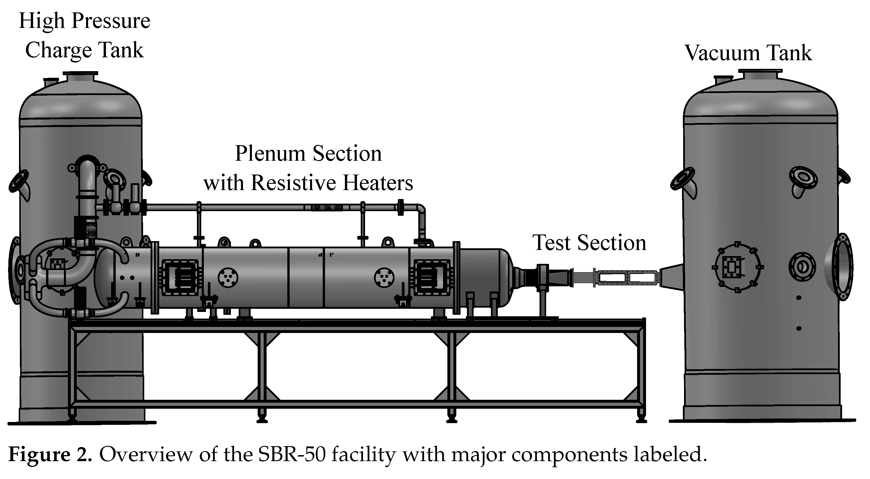
A general photograph of the SBR-50 is shown in
Figure 1. It consists of a high-pressure tank, plenum/air heater, nozzle, test section, diffuser, and low-pressure/vacuum tank. The test section can operate as a supersonic combustor, with the fuel injectors and electrical discharge generator flush-mounted on a plane wall or in cavity flameholder geometries [
15,
16]. The SBR-50 is also used for an active flow control research [
17,
18].
The SBR-50 facility features an Ohmic air heater installed in the plenum section. The air (or other gas if needed) is heated at stagnation pressure
before the run for several minutes up to a maximum of
K. At the beginning of the run, when the gate valve opens, gas rarefaction leads to temperature reduction in the plenum and test Section [
19]. To overcome this, additional valves open on the back side of the plenum, compressing the air in the plenum to maintain a constant pressure and ensure that test section temperature remains constant. The boundary between cold and hot air moves along the plenum section during the run working, similar to a virtual piston. The plenum section is designed long enough to provide a run time up to 1 s at flow Mach number
. To some extent, such a configuration could be treated as a combination of a blowdown scheme with a Ludwieg tube. For the SBR-50 facility, it is not known a priori how the plenum cold-hot air mixing at the virtual piston boundary affects the flow parameters’ stability.
A variety of methods are employed for the characterization of stagnation temperature in supersonic flows. The most simple direct method is a stagnation temperature probe consisting of a thermocouple near the end of a metal tube with side vents to increase the recovery factor. However, the use of this type of probe is challenging in short duration supersonic flows because the response time is long, typically on the order of second(s), and the recovery factor must be found by empirical calibration. A stagnation point heat flux probe [
20] has a much faster response time, down to the order of microseconds, but computing stagnation temperature from the heat flux of a semi-infinite body requires detailed calculations. Additionally, the method requires that the stagnation temperature be significantly higher than the initial temperature of the probe in order for appreciable heat flux to occur.
Stagnation temperature may also be indirectly obtained by measuring freestream static temperature or velocity along with Mach number, and then computing stagnation temperature using isentropic relations. Coherent anti-Stokes Raman scattering (CARS) is a commonly used method [
21,
22,
23,
24] for measuring both rotational and vibrational temperature in a wide variety of flows. However, the method is difficult to implement in most cases and requires specialized (and expensive) laser equipment. A multitude of techniques exist for measuring gas velocity, including laser Doppler velocimetry (LDV) [
25], particle image velocimetry (PIV) [
26], schlieren image velocimetry (SIV) [
27], femtosecond laser electronic excitation tagging (FLEET) [
22,
23,
28] and krypton tagging velocimetry (KTV) [
29]. However, PIV techniques in supersonic flows suffer from issues with seeding and particle slip. The laser-based tagging techniques posses insufficient accuracy and require specialized equipment and proper optical access. Since conventional schlieren methods are spanwise integrated, cross-correlation based SIV techniques are complicated by the need to distinguish the freestream velocity
from the convective velocity
in the side wall boundary layers, where
. An alternative and readily applied velocimetry method for freestream flow is laser spark velocimetry (LSV) [
30,
31], in which a laser-induced plasma (laser spark) is generated in the flow and convects downstream. The plasma luminescence may be tracked directly [
30], or the hot gas kernel created by the plasma may be tracked using schlieren visualization [
31].
In the excitation of the laser spark, the high electric field at the focal point of the laser ionizes the neutral gas, which then absorbs a fraction of the laser energy, creating a hot plasma that expands outward with a strong concomitant shock wave [
32,
33]. Due to the elongated shape of the laser beam waist, the hot plasma and the resulting SW is at first elongated rather than spherical. The dynamics of the shock wave and hot gas kernel can be approximated using the Sedov-Taylor [
34,
35] self-similarity solution for a strong explosion. The Sedov-Taylor solution assumes a strong shock and so is only valid while the Mach number of the shock wave is
[
32]. In the weak shock limit an extended blast wave solution is required, such as those of Refs. [
36,
37], while the blast wave continues expanding into the gas medium as a progressively weakening shock wave, the hot gas kernel reaches a final radius when the hot gas pressure equals that of the surrounding gas. As the pressure behind the shock wave decreases, the pressure gradient of the hot kernel is inverted and the kernel collapses to a degree, with the hot gas on the laser axis continuing to move towards the laser source and the surrounding hot gas forming a turbulent vortex ring around the jet [
38].
The objective of this work is perform SBR-50 flow characterization at two Mach numbers,
and
, with variable stagnation pressures and temperatures.
Figure 2 provides a basic summary of the facility. The flow temperature is measured by two different methods: direct measurements by a thermocouple and indirect measurements through LSV. A stagnation temperature probe is used to obtain qualitative stagnation temperature and its dynamics data. Complementary, an LSV method with schlieren tracking is used to obtain quantitative data on freestream velocity. Mach number is independently measured using a standard Pitot rake and the Rayleigh Pitot tube equation. The stagnation temperature is then computed using isentropic relations.
2. SBR-50 Description
The SBR-50 facility consists of a 1.9 high pressure charge tank, a 0.94 plenum, and a 5.6 vacuum tank. The plenum is double walled, with direct connection between the outer plenum section and the charge tank for filling the plenum and a spiral path connecting the outer and inner plenum sections which opens at the rear of the plenum. The plenum is wheeled and supported by two tracks on a steel frame so that the entire plenum section can by moved along its axis when not secured to the test section. A fast gate valve separates the downstream plenum head from a transition region and the nozzle section, which consists of two interchangeable 2D planar nozzle halves. To minimize large scale rotation when adding air from the charge tank to the plenum, the charge tank is connected to the plenum in four branches, each offset 90 degrees from the next with a 90 degree inlet to the plenum. Within the plenum are three sets of hexacomb flow straighteners to reduce vorticity and two sets of Ohmic heater banks with 12 heater elements each, total electrical power 67 kW.
Four valves, one on each connecting branch, control the time sequence when gas from the charge tank is flown into the plenum. Over the text, the wording is used when “back valves on” means that the back valves between the charge tank and the plenum section open at 0.1 s after the opening of the main valve, and remain open during the entire operation. The phrase “back valves off” means that back valves was not opening and no additional cold gas is supplied. In the “back valves on” operation, higher pressure gas from the charge tank pressurizes the hot gas in the plenum in a virtual piston configuration aiming for better stabilization of the pressure and temperature in the test section over the course of each run. This virtual piston concept is an alternative approach to a mechanical piston in the hope that adiabatic cooling due to volumetric expansion is reduced. In other words with a lesser similarity, it could be compared to a contact boundary in a Ludwieg tube configuration with a much larger gas volume involved.
2.1. Test Section
The nozzle is followed immediately by the test section, which has a cross section of 76.2 × 76.2 mm at the nozzle exit and a 1 degree half angle expansion on the top and bottom walls to account for boundary layer growth. Four 5 × 12 inch quartz side windows provide optical access to the test section. Two top and two bottom stainless steel wall inserts have 16 static pressure ports each. The inserts are removable to allow for the insertion of a variety of specialized test section articles. These removable inserts as well as a full schematic of the test section is provided in
Figure 3. The test section is connected to the vacuum tank through a diffuser, which has a 4 1/2 inch flanged fused silica window directly opposite the test section for optical access along the test section centerline. The vacuum tank is connected to a vacuum pump. Two 2 m long 95 mm square aluminum rails are joined and orientated orthogonal to the test section for the mounting of cameras and other diagnostic instruments.
2.2. Schlieren Visualization
Density gradients are visualized using a conventional refractor-based schlieren system. A high-power white LED (Luminus Devices CFT-90-WCS-X11-VB600) is powered at 40 A by a pulsed diode driver (PicoLAS LDP-V 240-100 V3.3) with external Peltier cooler (TE Technology CP-065 and TC-24-10). The broadband white light is collected and focused by an aspherical condenser lens (Thorlabs ACL50832U-A) and achromatic doublet (Edmund Optics 49-289-INK) and passed through an iris diaphragm. Two refractor lenses (Celestron Omni XLT 120) collimate and refocus the light. A vertical knife edge is place at the second focal point to visualize density gradients. The image is recorded by a high speed camera (Phantom v1611) with relay lens (Nikon 200mm f/4 AI). The high speed camera and diode driver are controlled and synchronized by a pulse generator (Berkeley Nucleonics 577). The LED optical pulse width is 100 ns with a repetition rate of 200 kHz. The exposure time of the high speed camera was setup to the minimum value of 300 ns: the LED optical pulse was triggered to be within this window.
3. Thermocouple Measurements
In an effort to characterize the temperature conditions inside the wind tunnel test section over the course of a run, a thermocouple probe was installed mid-stream. Temperature and pressure data was collected simultaneously over a variety of conditions in order to characterize the flow parameters and compare differing cases. For thermocouple measurements, the matrix of test conditions involved 300 K, 500 K, and 700 K nominal temperatures, Mach 2 and 4, higher and lower pressures
and
bar, and charge tank back valves on and off.
Table 1 displays exact information regarding pressure conditions used.
The difficult task of measuring flow temperature using a thermocouple involves recovering the fluid temperature from a measurement of the thermocouple junction’s temperature. When trying to measure flow temperature, the total error can be divided into velocity error, conduction error, and radiation error. Velocity error refers to the fact that the probe cannot recover all of the kinetic energy of the flowing gas as thermal energy. The ratio of kinetic energy recovered as thermal energy can be expressed as the recovery factor
where
is the indicated temperature at the junction,
is the free stream static temperature, and
is the actual stagnation temperature. Choosing the entrance to vent area ratio of the probe determines the velocity of gas over the probe tip, and can greatly impact the recovery factor and major source of error. For example, decreasing the velocity may reduce velocity error, but it also reduces convective heat transfer coefficients and thus leads to a larger conduction error. With regard to radiation errors, the thermocouple receives radiation from both the outer probe shield as well as some fraction from the test section walls as governed by the Stefan Boltzmann law
. In this setting radiation error is negligible compared to other errors, but by setting the probe tip further inside the shielding, the area of the colder tunnel walls that the tip sees is small compared to area of the hotter walls of the probe shielding. All these considerations were taken into account when designing the thermocouple probe as well as balancing robustness and practicality [
39].
At the expected temperature ranges inside the test section a type K thermocouple provides a very close to linear response. The size of the thermocouple was selected to balance the response time with robustness. In this case, a bead-welded thermocouple with a bead diameter of 1.2 mm was selected to provide the fastest response times possible without having to worry about the probe breaking under harsh flow conditions. The probe was mounted inside aluminum tubing. The inside of this tubing was coated with insulating paint near the probe tip to prevent shorting out the probe. For the details on the design and mounting of this probe see
Figure 4. The probe tip was set back inside the tubing by about 4mm and a small notch was cut in one side of the tubing behind the probe tip to act as a vent and increase the recovery factor.
Voltage data was collected with a Teledyne LeCroy HDO6034A-MS HDO6000A High Definition Oscilloscope and the known room temperature was used as the reference temperature. Since the thermocouple voltage amplitude is only a few millivolts, the voltage data is naturally quite noisy and was processed using a series of filters to mitigate this and generate a smooth calculated temperature time series. First a 60 Hz notch filter was applied with the goal of removing noise generated by surrounding electronics. Then, a third order digital Butterworth lowpass filter with a cutoff frequency of 0.0003 half-cycles/sample or with our 0.5 MHz sampling rate, 75 Hz. Last a rolling window average was applied over each 0.1 s. The voltage data was converted to temperature using a Type K thermocouple voltage response reference table and assuming a linear response in the operating region according to
where
R is the response coefficient and
is the reference temp which was room temperature [
40]. Note that none of computed temperature data presented in this section is strictly quantitative without proper calibration in well-certified flow conditions, but results provide a qualitative match and are generally representative of the actual temperature dynamics. Processed data is presented in
Figure 5,
Figure 6 and
Figure 7.
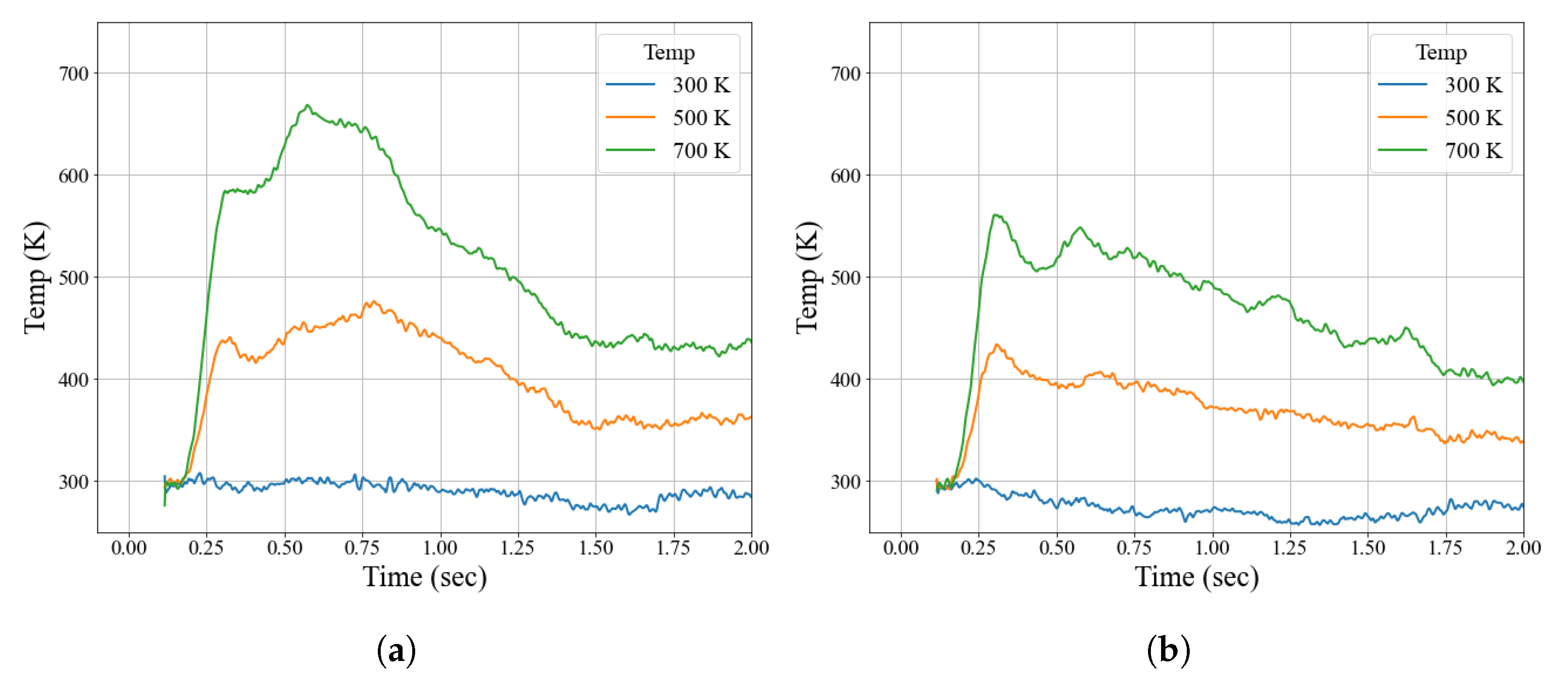
Comparing runs with the back valves on versus back valves off demonstrates that, in general, the facility is operating as designed. Examination of
Figure 5,
Figure 6,
Figure 7 and
Figure 8 demonstrates that keeping the valves closed introduces cooling due to the pressure drop whereas using the valves allows the plenum to push air out at a consistent temperature. According to
Figure 7, temperatures are higher at higher pressure runs, however, this discrepancy is largely due to the increase in thermal recovery factor of the probe at higher pressure due to increased convective heat transfer. The pressure jump at t = 1.7 s corresponds to the gate valve closure and supersonic-to-subsonic flow transition. Examination of
Figure 8 reveals the cooling and overall lower flow temperatures that occur when the back valves are off, while data is only presented for Mach 2, additional tests indicated that turning the back valves off introduced a more severe cooling effect at Mach 2 compared to Mach 4 which is because the mass flowrate is significantly lower at
.
For simplicity, the output of thermocouple was assumed to be dictated by thermal transfer from the gas to the probe as subject to Newton’s law of heating/cooling,
where
r is the coefficient of heat transfer. Solving this initial value problem for a step change in temperature and accounting for recover factor
yields the measured temperature model
Without an empirical calibration under specific flow conditions, the recovery factor of this probe is unknown and thus is assumed to be unity during an initial data processing. This assumption in the model leads to measured temperatures that are lower than real values but still provide useful qualitative results. The temperature data were fit with this model using a thermocouple time constant of 0.7 s to examine over what time period this exponential fit matches the data. This gives information on how long the tunnel can hold a constant stagnation temperature as well as a rough extrapolation what this temperature is.
Figure 9 shows that flow temperature is roughly constant for about 0.7 s.
Figure 9 also shows that with the valves on the recorded temperatures are higher and a stable temperature is maintained in the test section for slightly longer. Predicted flow temperatures from extrapolation are always lower than the actual tunnel stagnation temperature. In part this is due to the imperfect recovery factor of the probe, but also these predictions agree with a lower than nominal value of
calculated by laser spark experiments presented in the following section.
4. Laser Spark Dynamics
For Mach 2 flow, the fundamental wavelength of a ns-pulsed 100 Hz Nd:YAG laser (Solar Laser Systems LQ 629-100) is frequency doubled to 532 nm, expanded from a beam diameter of 4.6 mm to 12.3 mm, and focused into the test section using an
mm fused silica lens. The 532 nm pulse energy is 70 mJ/pulse as measured by a thermopile power meter (Ophir 50A-PF-DIF-18). The post-laser spark hot gas kernel is visualized using the high-speed schlieren system discussed above with 200 kHz framerate, 100 ns optical pulse width, and a vertical knife edge. For increased energy deposition in the lower density Mach 4 flow, the fundamental wavelength of 1064 nm (170 mJ/pulse) is used and is focused into the test section with an
mm fused silica lens. Representative image sequences for schlieren visualization of the hot gas kernel in Mach 2 and Mach 4 flow are presented in
Figure 10, where
and
correspond to the time and
x-location, respectively, of the initial breakdown.
Figure 10a,b each contain 17 consecutive schlieren images of a hot gas kernel as it convects downstream in Mach 2 and Mach 4 flow, respectively, with flow from left to right.
The hot gas kernel is tracked as it convects downstream using a cross correlation based algorithm. Each individual schlieren image (the sub-images in
Figure 10) is summed along vertical pixels, and the resulting 1D signal is cross correlated with a function consisting of a single sawtooth wave. The cross correlation peak is determined with sub-pixel interpolation using a second order polynomial. This process is repeated for every schlieren image containing the hot gas kernel, and an
x–
t plot is constructed using the fixed time between images of 5
s. The velocity of the hot gas kernel is then simply the slope of the
x–
t plot. Representative results are shown in
Figure 11, where
Figure 11a is the
x–
t plot for the convecting hot gas kernel shown in
Figure 10a and
Figure 11b–d are the cross correlation results for the 90
s sub-image in
Figure 10a. Since the R-squared value for the
x–
t plot is typically
, the error in measured convective speed is small and can be neglected.
Mach number is calculated from static pressure and Pitot tube pressure collected at 800 Hz by a multi-channel pressure scanner (Scanivalve MPS4264) using the Rayleigh Pitot tube equation. The results are presented in
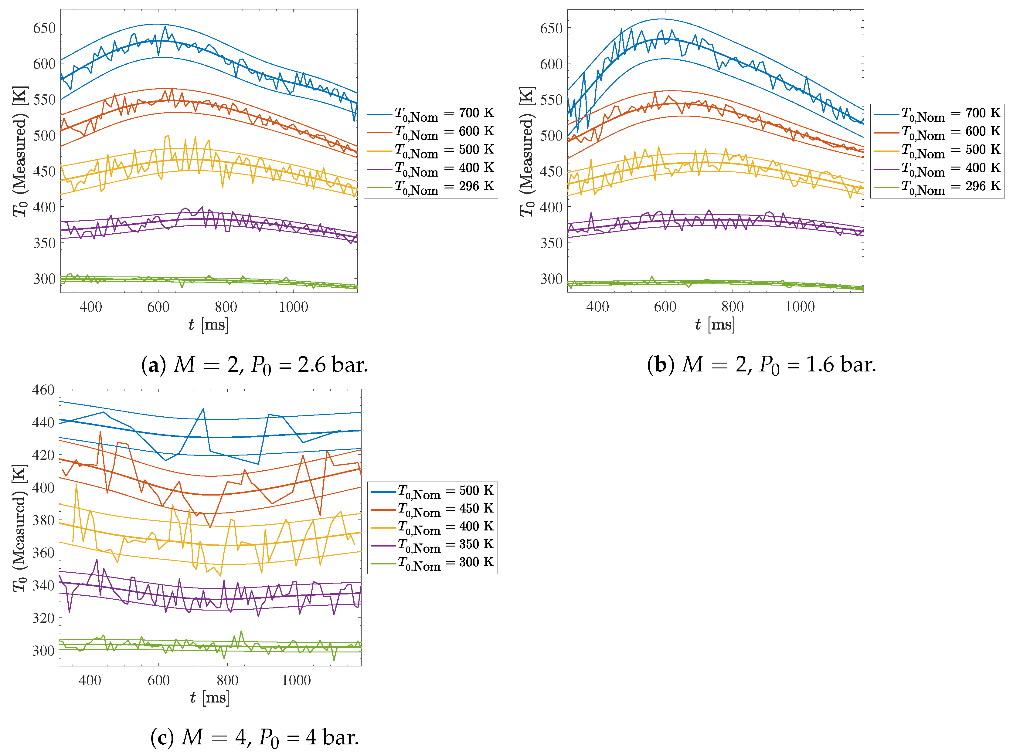
Figure 12. Stagnation temperature is computed using isentropic relations, and is presented in
Figure 13a,b for Mach 2 flow and in
Figure 13c for Mach 4 flow, where
corresponds to the time of tunnel start. For greater accuracy at high temperatures, the results at nominal stagnation temperatures of 600 K and 700 K in
Figure 13a,b are five run averages, with the standard deviation computed using the data of all five runs. Due to the low gas densities at Mach 4, the laser spark is formed only sporadically at high stagnation temperatures when the gas density is lowest. Therefore, fewer data points are included in the high temperature Mach 4 results, and the nominal stagnation temperature is limited to
K in
Figure 13c.
In
Figure 13, it is observed that stagnation temperature is relatively constant throughout the steady-state runtime of the facility, which is about 400–900 ms for Mach 2 flow and 400–1200 ms for Mach 4 flow. However, there are fluctuations in stagnation temperature that increase as the nominal stagnation temperature increases, which are thought to be due to incomplete mixing of gas within the plenum. Additionally, the average calculated stagnation temperature shown in
Figure 14a deviates from the nominal value as the nominal stagnation temperature is increased. It is hypothesized that this reduction in the calculated stagnation temperature is caused by the mixing of a relatively colder gas into the hot gas supplied by the plenum. This colder gas may originate from either a zone of high wall heat transfer or an imperfect seal between the plenum core and the helical cooling channel surrounding the plenum. The magnitude of the difference between the nominal and measured stagnation temperature is
where
is the ambient temperature and
for Mach 2 flow and
for Mach 4 flow.
5. Numerical Navier–Stokes Simulation
Numerical simulation of SBR-50 operation in different modes was performed using FlowVision 3.12.04 CFD software with the purpose of understanding the process of cold-hot air mixing at the virtual piston boundary and how the plenum configuration affects the stability of flow parameters. The simulation was based on the solution of the three-dimensional unsteady Reynolds averaged Navier–Stokes equations accompanied by the
turbulence model. The geometry of the simulation test section corresponds to the experimental one and the calculation domain includes the either the full setup including high-pressure charge tank, plenum, honeycombs and nozzle as in
Figure 15 or the symmetric half part of plenum, honeycombs and nozzle for more detailed temperature dynamics analysis as in
Figure 16. The full geometry was used to analyze the influence of slight deviations from symmetry, the real solenoid valve opening, and for determining the total pressure drop between charge tank and plenum. The second geometry was used for the simulation of SBR-50 operation with the virtual piston. In the half geometry, the symmetry condition was set to the vertical symmetry plane. No-slip conditions, adiabatic conditions, and wall functions were used on all other walls. The outlet boundary of nozzle was set to a free supersonic flow exit. The operation of the gate valve and solenoid valves were simulated using the “moving bodies” function of FlowVision, and in this approach the mesh around moving bodies is rebuilt at each time step. In this simulation, the gate valve opens with constant velocity from 0 to 0.2 ms, and solenoid valves open with constant velocity from 0.05 to 0.08 ms. Additionally, the temperature dynamics at a point directly at the center of the nozzle exit are compared with measured thermocouple data recorded from a point slightly downstream of the nozzle as shown in
Figure 17. In the used 3D URANS numerical method in conjunction with the k-
-model the grid independence was previously tested for similar tasks. The grid near the walls was based on the
appropriate for k-
-model (30 <
< 150). The grid in the flow volume allows for all large-scale features of the flow to be resolved. The software routine used allows the grid to be changed at any calculation step using adaptation (one cell splits to 8 at one level of adaptation and the number of levels is limited only by available RAM). The short period, when cold air is injected from charge tank, and the time period, when jet formation is possible inside the plenum, were simulated at different levels of adaptation to ensure the independence of large-scale features in the flow from the grid size or adaptation level.
Simulation results indicate that the boundary between hot and cool air inside the plenum experiences significant distortion as is seen in
Figure 16. These distortions could lead to unpredictable fluctuations in the stagnation temperature during a tunnel run, but expecially near the end of the run. When the back valves are open, air from the charge tank at room temperature pushes heated air out of the plenum but tends to form cold air jets near the centerline of the plenum as shown in
Figure 15. The presence of these cold air jets inside the plenum due to the introduction of cold higher pressure air from the charge tank back valves is a possible explanation of observed temperature fluctuation in stagnation temperature computed from laser spark measurements. As it is seen from numerical simulation, the delay between the first portion of cold air in the nozzle and main onset of cold flow could be about 0.25 s. One reason for the cold jet formation in the plenum in front of the main hot-cold boundary is the high speed of injected air coming from the charge tank. It is expected that further optimization of the cold air supply system could prevent such cold air jets and provide an increase in the duration of stable flow parameters from 0.45 s to up to 0.7 s at discussed operational parameters.
Figure 17 compares the simulation result with the data acquired by thermocouple and by the laser spark velocimetry. In both simulation and experiment, runs with the back valves closed lead to immediate expansion cooling after the gate valve opens, and runs with the back valves on lead to slight heating from initial over-compression. The data for the valves on operation mode prove the concept of the virtual piston. Additionally, on one side, data provides reasonable validation for these simulations, as key flow behaviors are matched by experimental results. On another side, an obvious discrepancy has to be discussed. A reasonable explanation is that the temperature data were extracted from indirect measurement datasets.The thermocouple data is computed with an assumed recovery factor of 0.9 in accordance with available literature suggesting that total temperature probes of this design in similar conditions demonstrated recovery factors ranging from 0.89 to 1.02 [
41]. The temperature values were recalculated by a differentiation procedure. Taking into account that the thermocouple time constant is close to the run duration, some error could be assumed. For the laser spark dataset, the gas temperature is recalculated from the direct gas velocity measurements. Because T is proportional to
, a small fluctuations in
v lead to clearly visible fluctuations in T. In simulations the gas temperature in the plenum distributes itself uniformly, while in the real facility, the near-gate valve portion of the plenum is not heated. This leads to significant difference in simulated and measured temperature values at t = 0.3–0.4 s.
A deviation in the geometry of internal elements in the plenum, such as an installation of a blocking disk near the plenum axes, affects the hot-cold gas mixing and an axial cold jet appearance in a significant degree. This opens a window for a further optimization of the flow parameters, including the duration of a steady state of the flow. In general, a manipulation of the timing of the back valves and the charge tank pressure allows for the ability to generate a flow field with time-variable predefined parameters, introducing an additional flexibility to the facility operation.
6. Conclusions
The supersonic facility SBR-50 at the University of Notre Dame is used for research efforts studying supersonic combustion and plasma-based flow control. The facility provides Mach number M = 2 and 4 flow with the total pressure 1–4 bar, stagnation temperature 300–775 K and typical duration of the steady-state flow 0.5–2 s. For the temperature control, an Ohmic gas heater is installed in a long plenum section. This manuscript describe some results of the flow characterization, specifically the dynamics of the gas temperature. Two measuring methods were applied for collection of a detailed dataset: thermocouple measurements, and schlieren-based thermal mark (laser spark) velocimetry.
The general conclusion resulting from these measurements is that the facility original schematics (virtual piston in the plenum concept) allows for a longer operation with a relatively constant stagnation temperature compared to a constant plenum volume with adiabatic cooling of the stored gas. At the same time, results demonstrate a significant level of temperature perturbation, which needs additional clarification. Another effect observed and under further analysis is a notably lower stagnation temperature measured at M = 2 and M = 4 than the one measured in the plenum. This effect is attributed to an uneven gas temperature distribution over the plenum section.
The numerical simulation indicates that the gas temperature in the test section could potentially equal the plenum gas temperature for as long as t = 0.45 s. Additionally, it shows that an optimization of the plenum geometry and the gas premixing in the plenum could resolve some of the issues with the gas temperature dynamics. These results also demonstrate that the virtual piston concept implemented by injecting air through the back valves stabilizes pressure and temperature values (variations less than 5%) in the test section. It was noted that further optimization of the cold air supply system could extend the stable window of operation from 0.45 s to up to 0.7 s under explored conditions if the cold jet formed by the charge tank air supply is suppressed.


