1. Introduction
Over the last decade, Volume-of-Fluid (VoF) methods and their variants [
1] have gained popularity in the simulation of two-phase flows due in part to their mass conservative nature. Among these methods, the algebraic VOF methodology encapsulated in
interFoam has been available for a large number of years as part of the open source distribution of OpenFOAM and has attracted significant attention (A 10 March 2022 search in the Google Scholar database revealed 3030 sources that included the word “
interFoam” anywhere in the article). In this method, the effects of numerical diffusion are assessed based on a compressive interface capturing methodology that was improved by Ubbink and Issa [
2] and Rusche [
3] with contributions from Henry Weller. More recently, new and often more accurate VoF methodologies have been implemented in OpenFOAM, for example, the isoAdvector geometric VoF with reconstructed distance function [
4,
5], the addition of the geometric level set [
6], the improvement to volume fraction (
) advection in complex mesh topologies [
7], the implementation of a coupled level set VoF (CLSVOF) [
8], and the introduction of a capillary pressure jump modeling [
9], among other contributions.
Despite the availability of other VoF methodologies within OpenFOAM, or even other open source frameworks [
10],
interFoam continues to be a popular choice. It can be speculated that part of the reason for its continued use is the familiarity of the solver among its many users as well as the development of submodels within its infrastructure, which can pose a significant time investment for their implementation in other solvers. Regardless of the reason for its continued use,
interFoam has its weaknesses, with the most prominent being arguably the calculation of interfacial curvature,
. This has been known for some time [
11] and has spawned various flavors of numerical fixes.
It is well established [
1] that the major difficulty with a curvature calculation within a VoF methodology is the high degree of error associated with the calculation of second-order derivatives of the naturally sharp volume fraction field. With a higher degree of grid refinement, the volume fraction field becomes progressively sharper, which can lead to a lack of numerical convergence for curvature predictions. Within the two-phase flow community, a common procedure for addressing this error is the use of a level set function,
, which is much smoother than
and can subsequently provide more accurate curvature predictions. This combination of
with
has been in existence for quite some time [
12] and has also been adopted within OpenFOAM, for instance in the work of Ferrari et al. [
7], Bilger et al. [
9], Albadawi et al. [
13], Menon et al. [
14], Kassar et al. [
15], Elsayed et al. [
16], Vachaparambil and Einarsrud [
17]. More explicitly in Ferrari et al. [
7], Albadawi et al. [
13], Menon et al. [
14], the level set is initially constructed from the
field, namely by an equation of the form
, where
is related to the local grid spacing,
. Subsequently, this initial
is reinitialized through the solution of a Hamilton–Jacobi equation, resulting in a signed distance function, which is then used to compute curvature. In other work [
9,
17], the
field is smoothed out before calculating curvature. Other alternatives include the construction of a uniform voxel mesh followed by isosurface triangulation [
16] or the representation of the interface by a cloud of points [
15], both of which are used to generate more accurate predictions of
.
The present work aims to examine the result of improvements to curvature estimation within interFoam. In contrast to previously published works, the evaluation exercises considered are more relevant to sprays and hydrodynamic breakup dynamics than bubbles or similar configurations. Particularly, the addition of the Rayleigh breakup problem and a 2-phase shear instability solved analytically through the Orr–Sommerfeld temporal analysis is aimed at these types of breakup scenarios.
Our approach is similar to the works mentioned previously in constructing a
field from the
field and computing curvature from
. However, there is a distinguishing characteristic in the present work in that
was created from a dual treatment that treats interfacial cells (cells containing the
isosurface) differently from the remaining cells. The motivation for this dual treatment lies in the erroneous displacement of the interface that results if the Hamilton-Jacobi reinitialization solution is applied in a domain that includes interfacial cells (cells that contain a segment of the interface). This problem has been documented previously [
18,
19] and it results from the propagation of information from the wrong side of the interface for some interfacial nodes. For the sake of providing an additional comparison, the common smoothing of the
field [
9,
17] is also implemented.
The contents are organized as follows. In
Section 2, a description is provided for the three curvature prediction methodologies. The evaluation exercises are presented in
Section 3 in order of increasing complexity. Since we are interested in liquid spray and droplet applications, the choice of exercises reflects this interest. A summary of our findings along with concluding remarks are presented in
Section 4.
2. Curvature Predictions
The curvature implementations and flow predictions reported in the present work employ the algebraic solver
interFoam (version 2.1.1). More recent versions of OpenFOAM under both ESI and foundation releases utilize essentially the same conventional curvature calculation found in OpenFOAM 2.1.1. A description of the liquid fraction transport, momentum, and pressure equation treatment can be found in [
11]. Since the focus of the paper is on interfacial curvature, the primary relevant parameter is the surface tension force appearing in the momentum equation. Its implementation is performed via the Continuum Surface Force (CSF) method [
20], namely
Here, the terms on the left-hand side (LHS) and center correspond to the analytical expression of the surface tension force exerted over an arbitrary space
. The interface is denoted by
(tacitly assumed to be temporally evolving), the curvature is denoted by
, the surface tension coefficient is denoted by
(treated as constant), the unit interface normal is denoted by
(oriented from the
gas to the liquid dictated by the direction of
), and the 3D Dirac Delta function is denoted by
. Its numerical treatment via the CSF is given by the term on the right-hand side (RHS) in Equation (
1), where the local curvature is defined as
Since the present development is made within the framework of
OpenFoam, its existing finite volume discretization is utilized. In particular, for an arbitrary scalar field
and vector field
, the following gradient and divergence approximations are employed:
In these equations,
corresponds to the space occupied by some computational cell
i and
is its respective volume. The corresponding surface area of cell
i is given by
. Quantities pertaining to
cell centers are denoted with subscript i, and
quantities pertaining to face quantities are denoted with subscript
f. The product of the surface area of the cell face
f (associated with cell
i) and the corresponding
outward unit vector is given by
. Equations (
3) and (
4) come directly from the Gauss Divergence Theorem and its gradient analog along with the application of the mean value theorem for definite integrals.
2.1. Standard Calculation (-Based)
The standard method or -based method is the native method present in interFoam. Even though the current version being employed is 2.1.1, other versions, including more recent ones such as ESI Openfoam-v2006 and OpenFoam Foundation version 6, continue to employ the same formulation. In the -based method, the curvature is computed as follows:
Cell-centered liquid fractions are linearly interpolated to the faces, i.e., .
The computation of
is performed using Equation (
3), with the scalar function
.
Normal vectors are calculated via
where
is a small scalar and its inclusion is to avoid division by zero. Calculation of
employs Equation (
3).
Cell-centered values for are linearly interpolated to cell faces, i.e.,
Having face values for the interface normal, the curvature is calculated using Equation (
4), namely
The aforementioned framework is part of OpenFoam and works for general polyhedra, i.e., it is not limited to structured grids.
2.2. Diffused -Based Calculation (-Based)
It is understood [
21] that due to the sharp nature of
, taking second-order derivatives to compute curvature leads to gross errors. One obvious alternative for reducing the magnitude of the error is to smooth out the
field. As noted in the Introduction, some authors [
9,
17] smooth the field by filtering
or the curvature within OpenFOAM. In the review article by Popinet [
1], he cites these methods as obsolete since newer methodologies offer better results. In this work, this smoothing methodology is used principally to provide another comparison data point against the standard method and the
-based method discussed below. However, rather than explicitly smoothing
or filtering the curvature, in the present work, the smoothing is applied by solving an unsteady diffusion equation for the liquid fraction over a specified number of time steps. The process is as follows:
Initialize
with the
field at some arbitrary time level
n, i.e.,
where
is pseudo time.
Advance
through the solution of
where
is the diffusion coefficient. Since the aim is to smooth the initial liquid fraction field over a length scale
, the associated total computation time is
. With such a short computation time, the choice is to employ an explicit methodology. The stability criterion in 2D is
and in 3D is
; hence, at most,
time steps are required. Numerically, the solution is advanced via
Normal vectors at the end of the previous calculation are computed via
Cell-centered values for are linearly interpolated to cell faces, i.e.,
Curvature is calculated based on Equation (
4) as
2.3. Distance-Based Calculation (-Based)
Motivated by the tradition of coupling level set with VoF to improve curvature estimate, in the present work, we similarly create this signed distance function,
. As previously discussed in the Introduction, the solution of the reinitialization equation at interfacial cells causes the interface to be erroneously displaced within these cells. Hence, the present approach is implemented in two steps, namely (i) interface reconstructions at interfacial cells [
22] and (ii) the solution of Hamilton–Jacobi equation excluding interfacial cells.
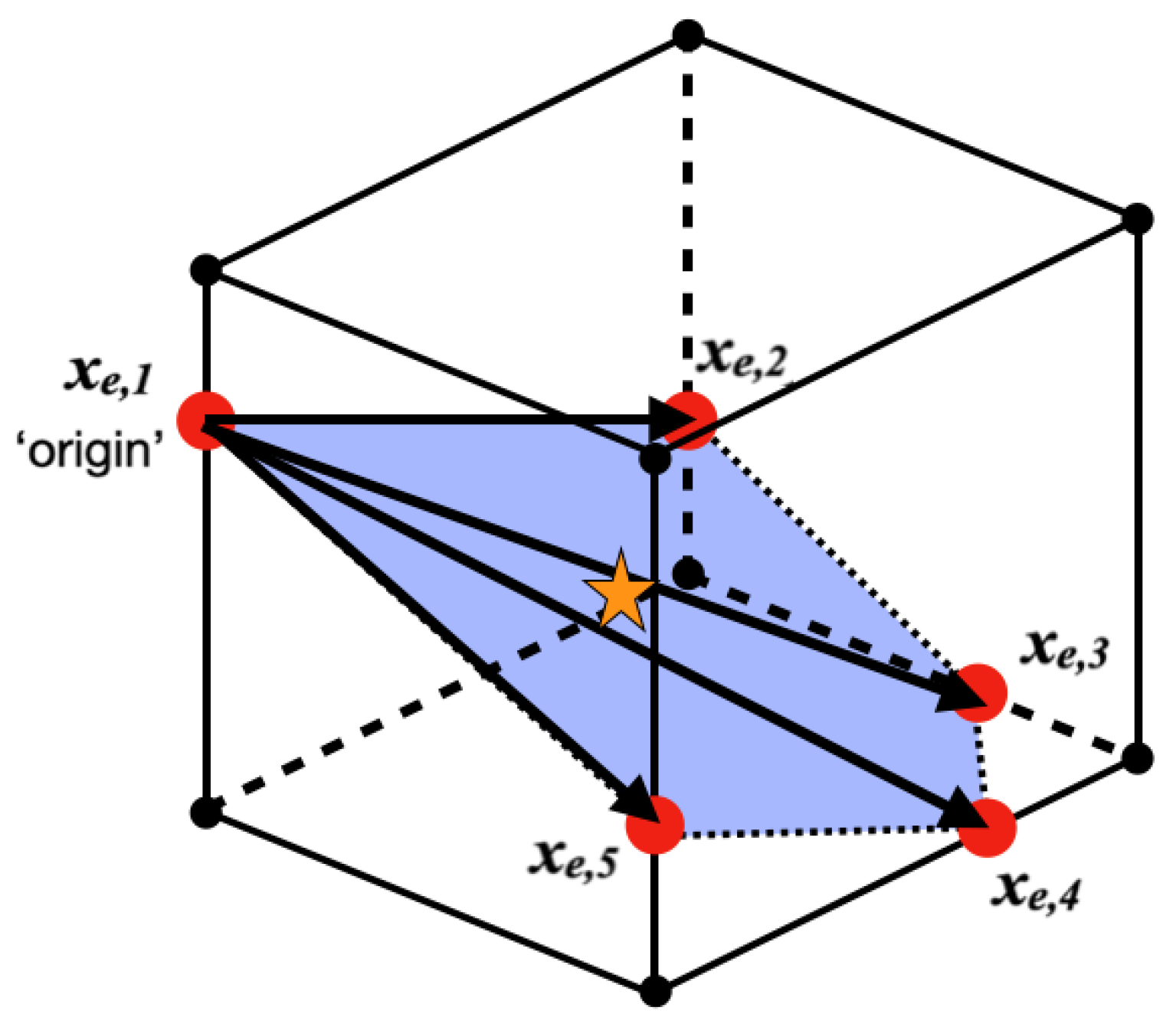
2.3.1. Interface Reconstruction
2.3.2. Hamilton–Jacobi Reinitialization
The solution of the reinitialization problem via the Hamilton–Jacobi equation is a well-established method for reinitializing a level set function to a distance function [
24]. It consists of solving
where
and
denotes a sign-function, i.e.,
for
,
for
, and
for
. An equivalent form of Equation (
16), which offers some insights into the behavior of this equation is
In this Lagrangian form, the propagation speed of is clearly shown as , and its evolution occurs in pseudo time. The process implemented in the current work is as follows:
3. Results
The performance of the three curvature estimation methods is examined among five evaluation exercises as shown in
Table 1. Since the main focus of the work concerns curvature improvement, which is directly related to surface tension, the choice of problems is, for the most part, heavily influenced by this effect. The only exception is the temporal interfacial instability analysis at a Weber number of 100 presented in
Section 3.3.
3.1. Laplace Pressure Problem
The Laplace pressure test is undertaken to isolate the accuracy of surface tension predictions. This case is governed by the Young–Laplace equation, namely , where the pressure on the liquid and gas side are, respectively, given by and . Here and in the remainder of the document, the liquid and gas phases are denoted by subscripts, L, and G, respectively.
In the present case, the exercise consists of a liquid 2D droplet in zero gravity having a radius
m, and
m
−1, densities
, viscosity
, and surface tension
yielding a Laplace number
The domain consists of a
square with the droplet positioned at its geometric center. The radius of the droplet is
. For boundary conditions, a zero gradient is imposed for
, a zero Dirichlet condition for pressure, and partial derivatives of all velocity components with respect to the coordinate normal for each boundary are zero. This is termed a zero gradient condition for velocity. Due to surface tension, a jump in pressure is immediately recorded, which initiates a transient. Since the calculation is performed well within the numerically stable regime and physically corresponds to a steady solution, the transient decays and an equilibrium condition is achieved. The examination of pressure jump is performed during this steady period, and consequently, the computations are executed to
consistent with previous studies in the literature [
11,
25].
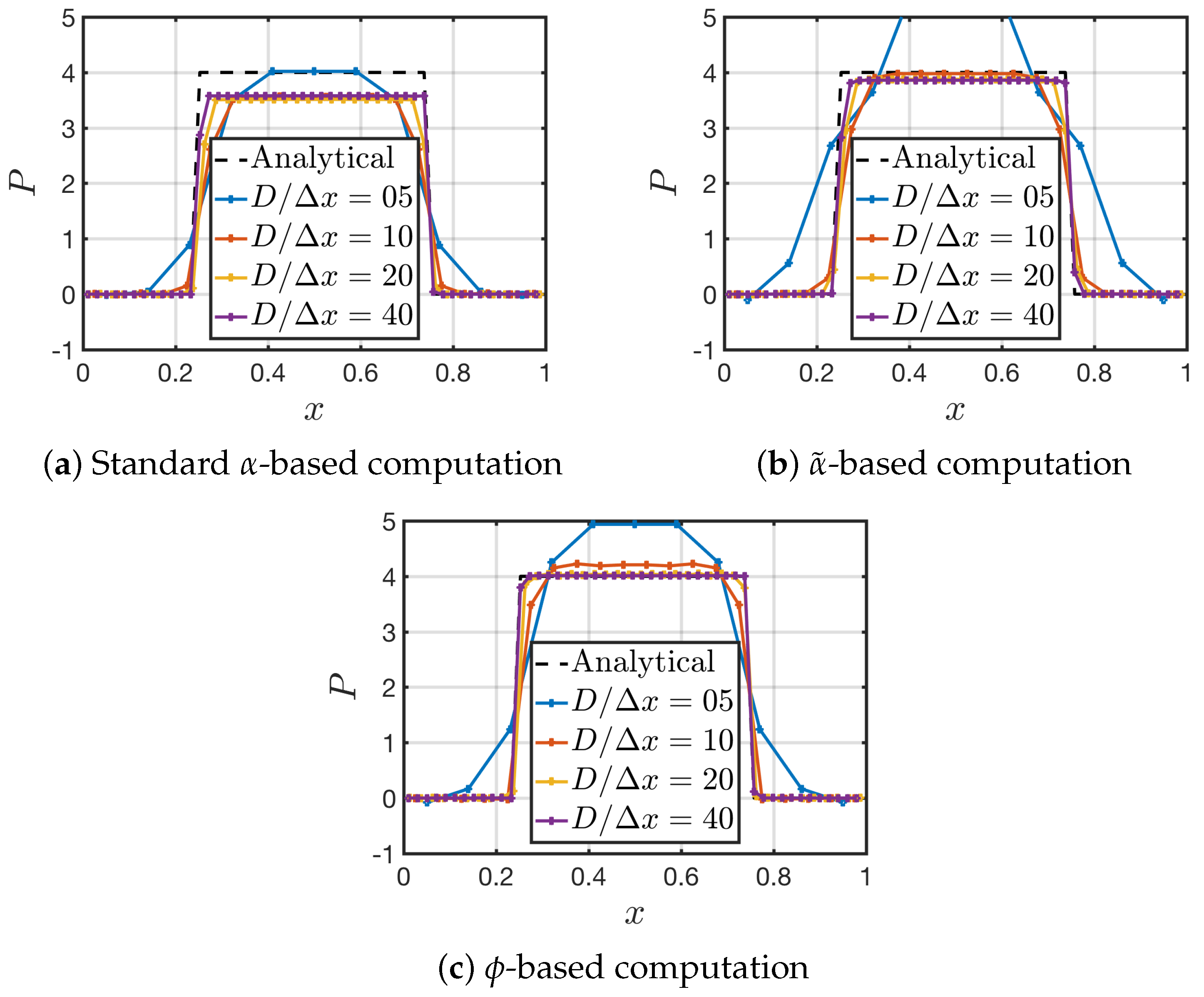
The pressure profile along the centerline is extracted and plotted in
Figure 2 corresponding to the three methods for computing
. In each plot, the analytical solution is provided along with predictions corresponding to four different levels of numerical resolution. For the standard
-based method shown in
Figure 2a, it can be seen that, upon refinement, the pressure inside the liquid converges to a value lower than the analytical value, in agreement with an earlier publication [
11]. This is a direct result of the poor curvature predictions, as expected. The pressure values improve for the other two methods, as seen in
Figure 2b,c. For the
curvature method shown in
Figure 2b, the results are noticeably better, leading to what appears to be an agreement with the exact values. For the
-based computation, the results show that predictions with a resolution finer than
are essentially indistinguishable from analytical values.
To quantify the degree of convergence, the Laplace pressure is computed for all three methods as a function of grid resolution
. This pressure is computed according to
where
and
are, respectively, the internal and external pressure to the droplet and are computed as follows
where
is the region given by
and
is the region given by
. The number of computational cells in each region is given by
and
. The reason for this choice of regions is to ensure that, with coarse level calculations, the interior and exterior domains are properly accounted for. The associated numerical error is
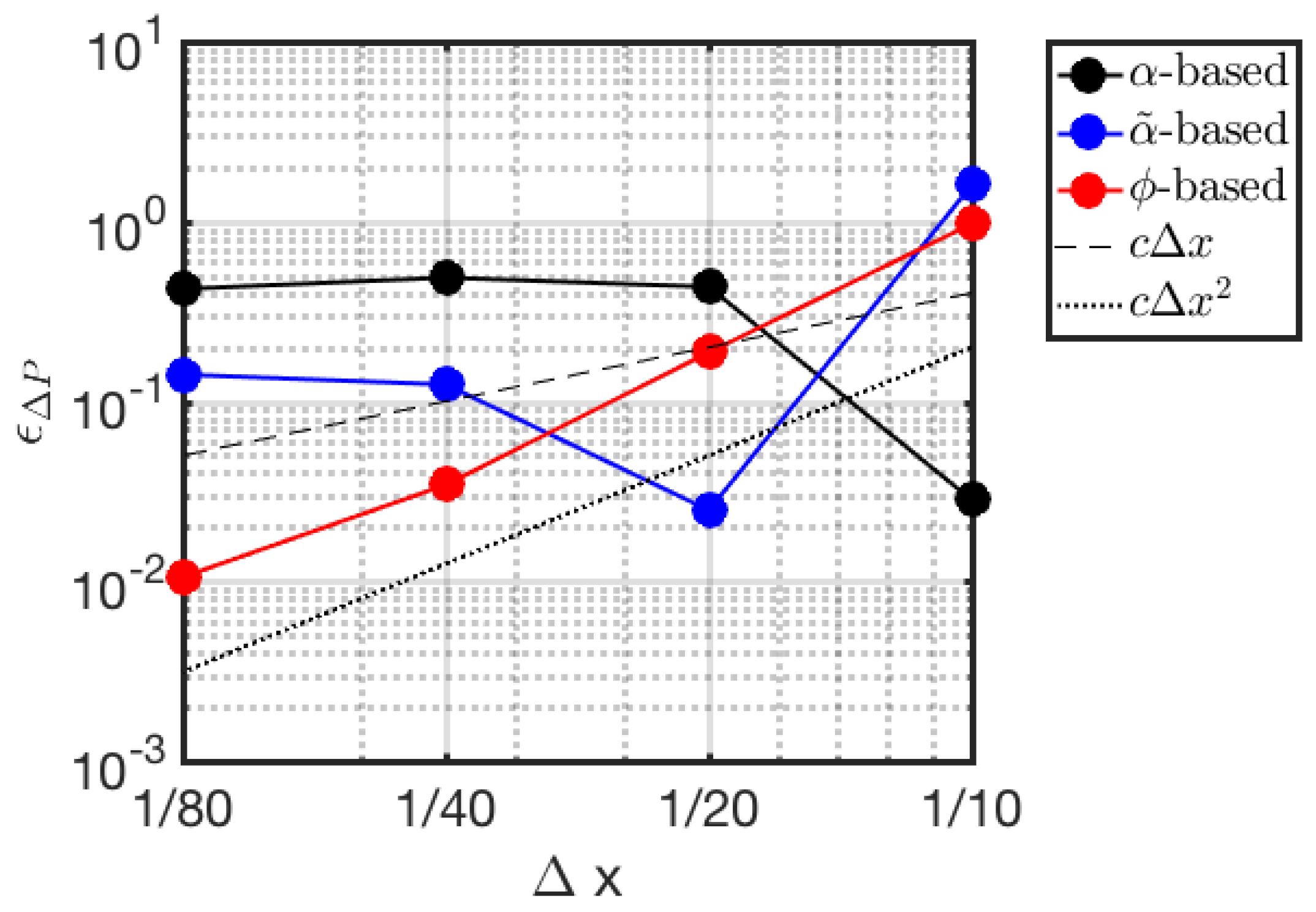
This error is calculated as a function of grid resolution in
Figure 3. Two reference lines corresponding to first- and second-order convergences are included as well. Beginning with the standard method, the predictions initially diverge and reach a plateau at an appreciable high level of error. No convergence is observed. For the
, the magnitude of the error is smaller; however, the method also lacks convergence. Lastly, for the
-based method, second-order convergence is achieved, and the method is superior to the previous two schemes for computing curvature.
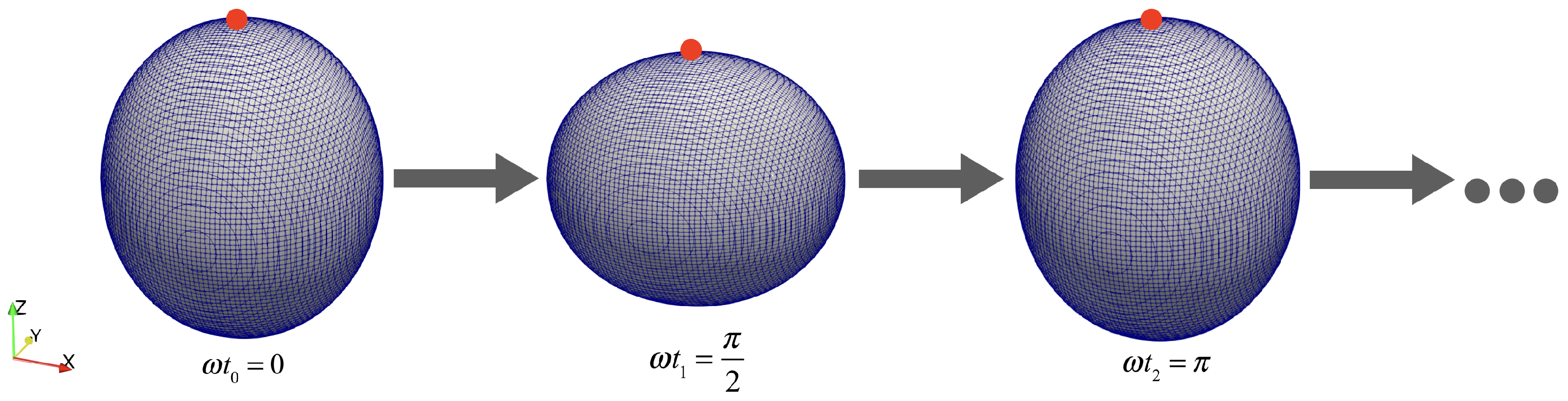
3.2. 3D Oscillating Droplet
This exercise consists of introducing a small perturbation on an otherwise quiescent spherical droplet under zero gravity, where the resulting motion is driven by surface tension. Thus, the present exercise aims to isolate the effects of curvature predictions in a dynamic environment. If the unperturbed radius is given by
, the initial surface of the droplet is given by
where
is the polar angle given by
and
is the distance of the interface from the center of the droplet at some
. An illustration of this problem is shown in
Figure 4.
In the present exercise,
m and the magnitude of the perturbation is
m. The departure from pure spherical form is described by the Legendre polynomial of second order,
. The droplet is positioned at the geometric center of a
domain. For boundary conditions, a zero gradient is assigned for
and pressure, and a no-slip velocity condition is imposed at all the boundaries. The densities employed are
and
; the viscosities are
and
, and the surface tension is
. This setup is the same as the one used by Patel et al. [
26] and the resulting Laplace number (
),
10,000, which is characterized by the dominant effect of the product of inertia and surface tension forces over the square of viscous forces.
In the work of Lamb [
27] (pg. 563), an analytical expression for the motion of the interface is provided. A more modern version of this expression can be found in Patel et al. [
26], namely
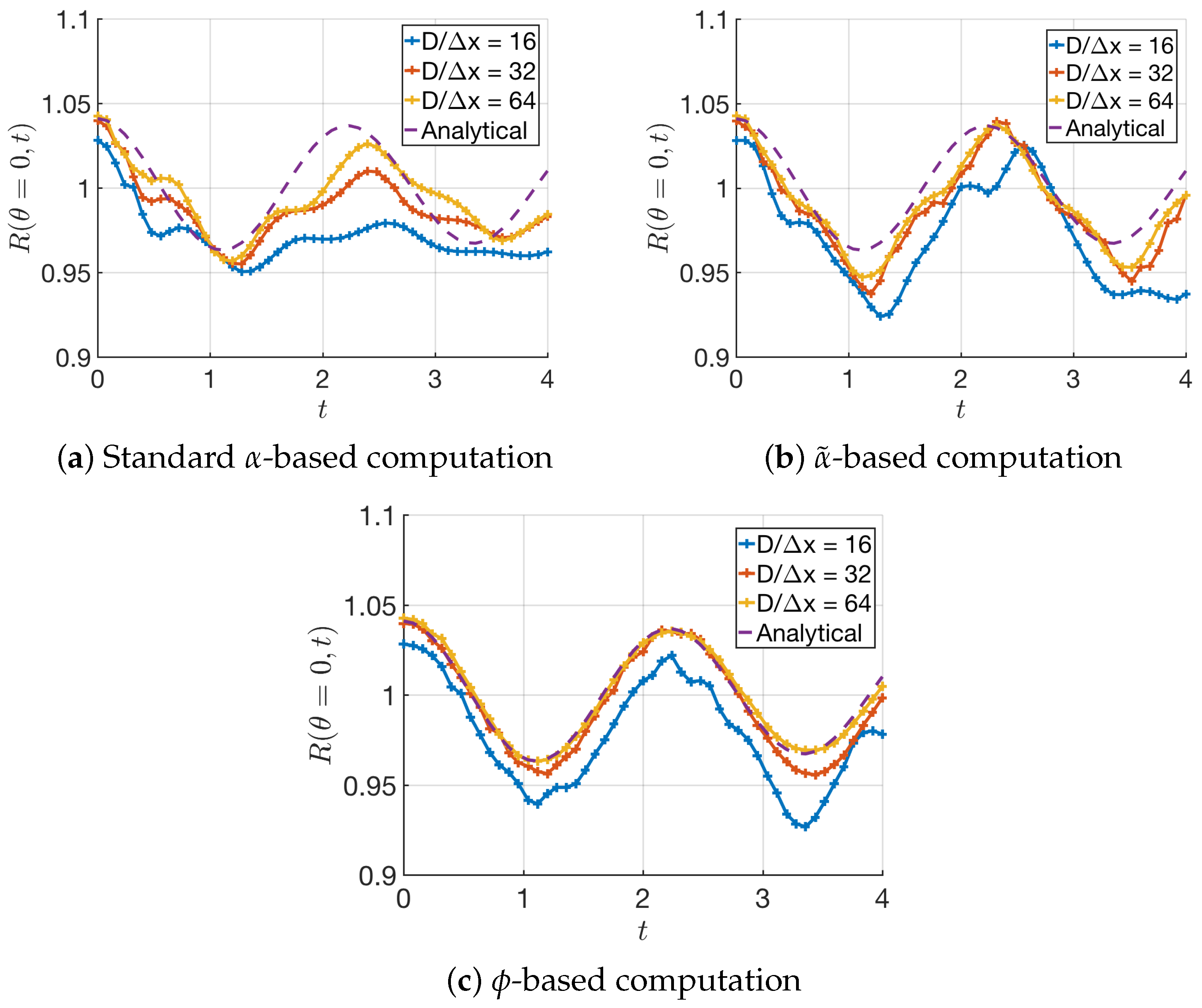
Predictions from the three curvature schemes are compared against this analytical solution, as shown in
Figure 5. The first observation is that predictions at different levels of resolution do not agree initially, i.e., at
. This is particularly the case for the coarser case, i.e.,
16, and is due to the degree of numerical error in identifying the interface (
contour). At higher levels of resolution, the agreement at
improves substantially. A second observation is that the solution from the standard
-based method contains erroneous harmonics that do not disappear even at the finest level of resolution. The agreement with the exact solution is far from encouraging. Employing the
-based method, there is some measure of improvement, but still, the numerical predictions contain anomalous oscillations. In the
-based method, anomalous behavior is slightly observed in the coarse case, but with higher levels of resolution, the predictions quickly match the analytical solution and no erroneous harmonics populate the predictions.
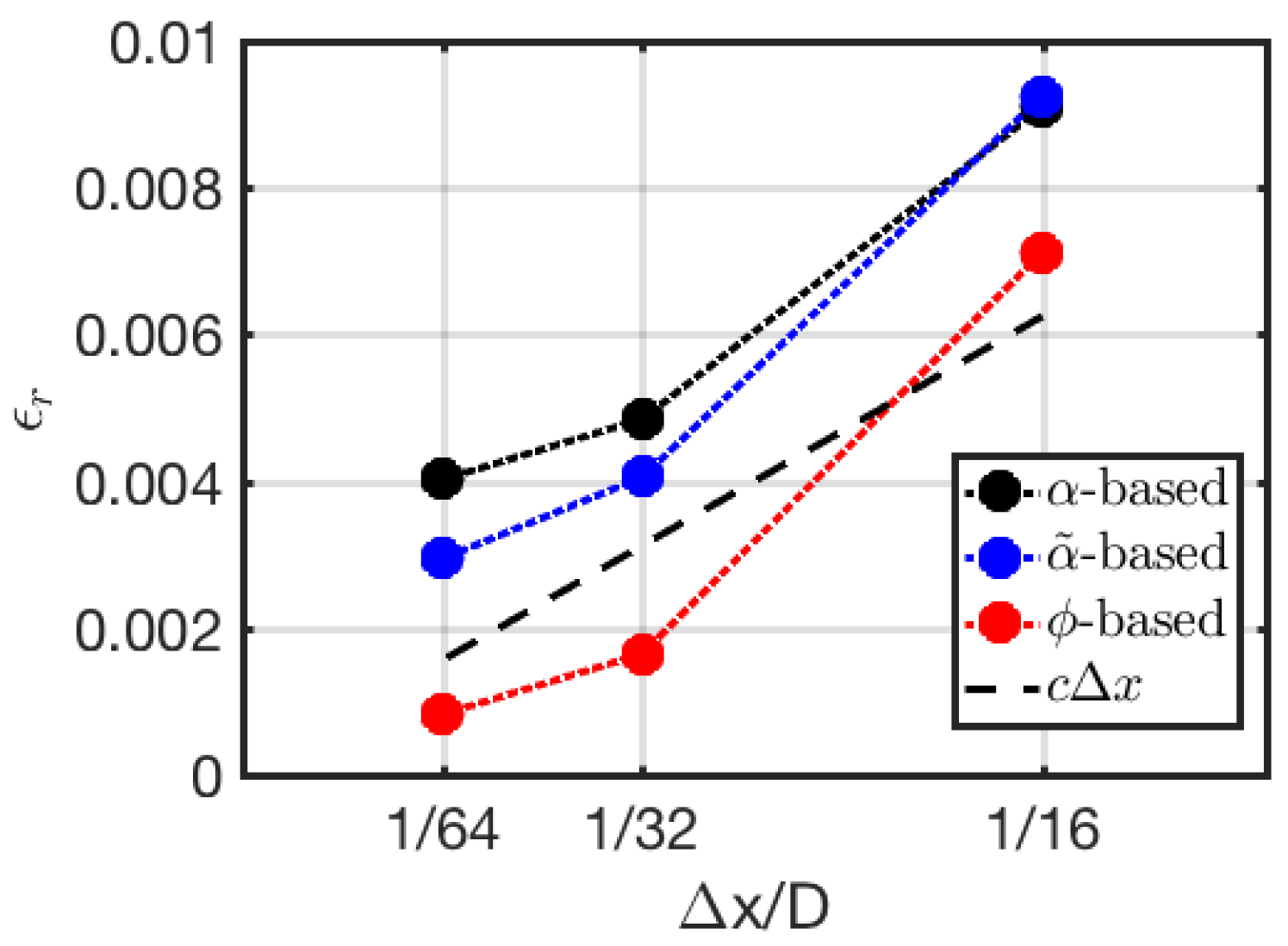
To quantify the level of performance, the following error metric is employed
where
is the discrete-time level and
is the total number of time steps. The numerical prediction for each method is denoted by
. As such, this error represents a time-averaged of the instantaneous deviation from the analytical solution. The results are shown in
Figure 6 as a function of grid resolution, and a first-order reference line (
) is provided. The observation made previously is confirmed, where it is apparent that the
-based method has a lower error magnitude compared with the other two methods. The convergence rate for all three methods is initially better than first-order accuracy but slows down at higher resolution levels. Interestingly, the standard
-based case shows convergence even though, visually, the result does not appear to be encouraging.
With the inclusion of dynamics, all three methods display numerical convergence, with the -based method having a consistent lowest magnitude of the error. However, the convergence rate for the -based method is no longer second order but has declined to approximately first order, most likely due to the associated errors involved in calculating momentum and displacement of the interface. It is interesting to see, however, that this added motion had a negative effect on the convergence rate of the most accurate method presented in this work but a positive effect in the less accurate methods. In fact, for this case, these methods have improved from having no convergence in the static case to convergence in the present dynamic exercise.
3.3. Shear Layer: Growth of Interfacial Instability
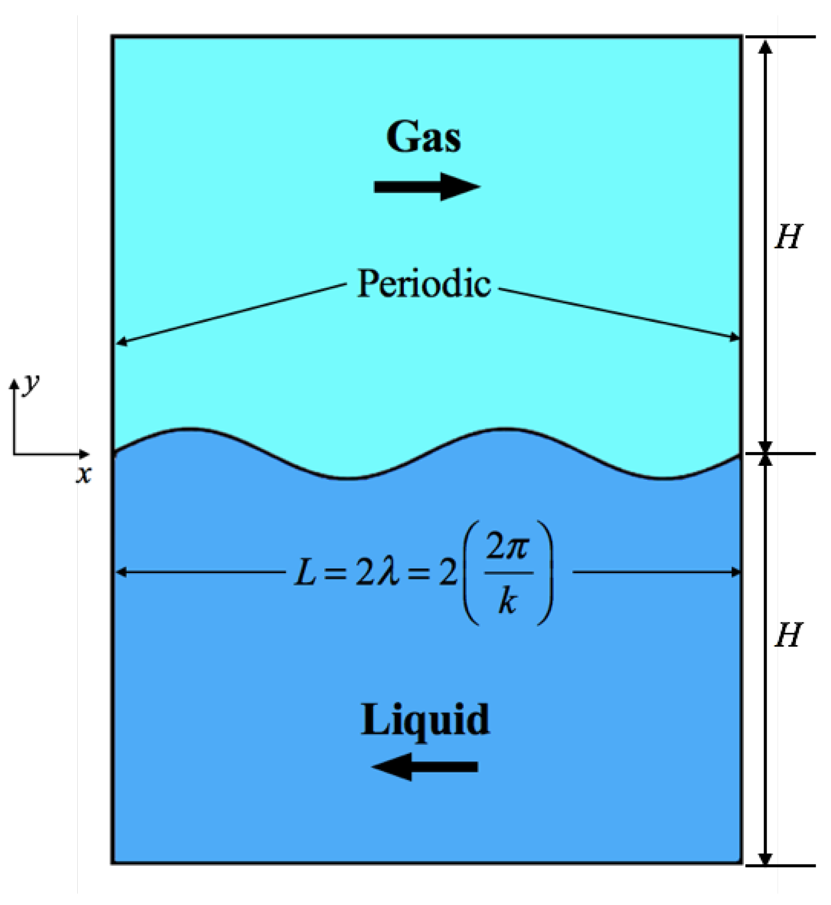
The two-phase shear layer is a fundamental fluid mechanics problem that is particularly relevant to atomization and spray formation and is often omitted in numerical tests for curvature predictions. This problem is illustrated in
Figure 7, and it consists of a gas and liquid stream that is characterized by a velocity difference leading to the establishment of a shear layer. Authoritative descriptions of the dynamics characterized by Kelvin–Helmholtz instability can be found in the text by Criminale et al. [
28] (pg. 39–42).
In the present work, a 2D temporal instability Orr–Sommerfeld calculation is employed, where a perturbation of wavenumber
(
is the wavelength) is imposed with periodic boundary conditions on the left and right sides of the domain, as shown in
Figure 7. On the top and bottom boundaries, a zero gradient is imposed for
and pressure and a slip condition is imposed for velocity. This slip velocity condition consists of zero gradient for velocity components, which are tangential to the bottom and top boundaries, i.e., x-direction, along with a zero normal velocity component.
In brief, the velocity field is decomposed as
where
is the base flow profile and
is the perturbation velocity. The base profile used in this exercise is
with values of
0.99
and
1
. These values can be obtained from the shear stress balance of the base flow field at the interface, which gives
. The perturbation flow velocity is described in terms of a stream function,
, as
where the stream function takes the normal mode form of
In this expression,
extracts the real part of its argument, the eigenvector
, the input wavenumber
, and the complex wave speed
. The imaginary part of the wave speed,
, is responsible for the growth or decay of a given mode. The normal mode expression for the stream function is substituted into the Orr–Sommerfeld equation in combination with the gas–liquid interfacial constraints, namely continuity of normal and horizontal velocity and balance of tangential and normal stresses. Details are provided in [
29]. The resulting linear system is a generalized eigenvalue problem that is solved for (
), where
is the y-profile of the stream function and
c is the complex eigenvalue.
The predictions from the Orr-Sommerfeld system are compared in this exercise to those obtained from the VoF employing the aforementioned methods for estimating curvature. The domain is 2D of length
and height
6 m. The fluid densities are given by
and
, the viscosities are given by
and
, the surface tension coefficients are given by
and
, and
. The associated Weber number for this exercise is defined as
hence, the above two values for the surface tension coefficient correspond to two cases considered, i.e.,
and
.
In the calculations, the grid refinement is set to
0.011
to ensure that the small initial perturbation is sufficiently resolved. A convenient way to track the growth of the perturbation is to compute its kinetic energy. For the type of periodic domains considered here, this method bypasses the need to compute the perturbation growth by meticulously trying to fit the interface at various times during the growth process. The perturbation kinetic energy,
, is computed as
where
,
(liquid domain),
(gas domain) (see
Figure 7), and
. It can be shown [
29] that
, where
and
are constants. Thus,
and the value of the growth rate,
, can be readily obtained from plots of this kinetic energy ratio. From Equation (
38), the growth rate is related to
c via
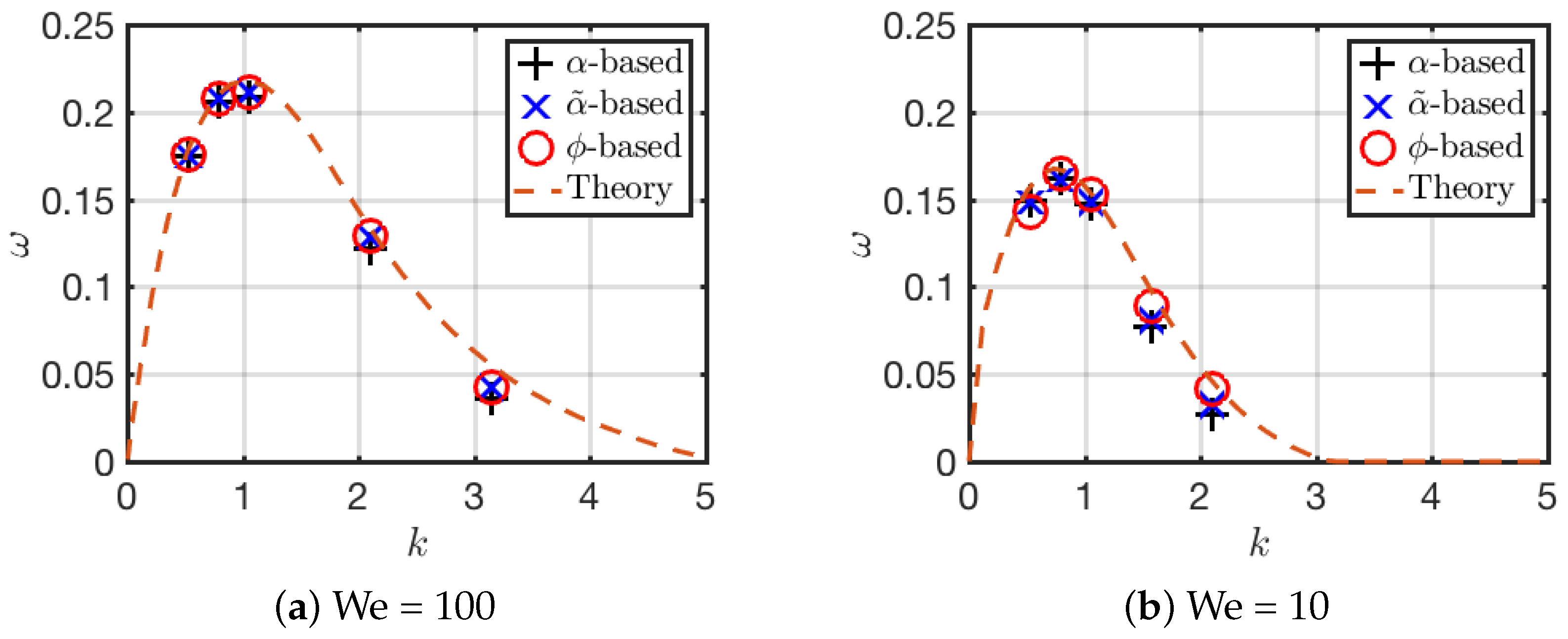
. The comparisons between VoF predictions and linear stability results are shown in
Figure 8 and in
Table 2 and
Table 3. In the tables, the error is calculated as
, where the normalization factor is
, i.e., the maximum growth rate. This normalization factor is employed to ensure that the same factor applies to all errors calculated. For instance, a normalization factor equal to
would result in an exaggerated reporting of the error at high wave numbers even for cases where the error is relatively minor due to the growth rate approaching zero in this part of the wave number domain.
Overall good agreement is observed between the simulation results and the theoretical prediction with the three methods. Due to the stabilizing action of surface tension, the cases for exhibit a slower growth rate than those at . At higher , all errors are within 5% but increase to a maximum of 12.4% at . This is not surprising since the influence of surface tension and, thus, the effect of curvature error increase with lower values of . Additionally, the magnitude of the error decreases when transitioning from the standard -based method to the -based method. However, this improvement is not as dramatic as in the previous exercises. The predictions are reasonably good even with the standard method, particularly at 100.
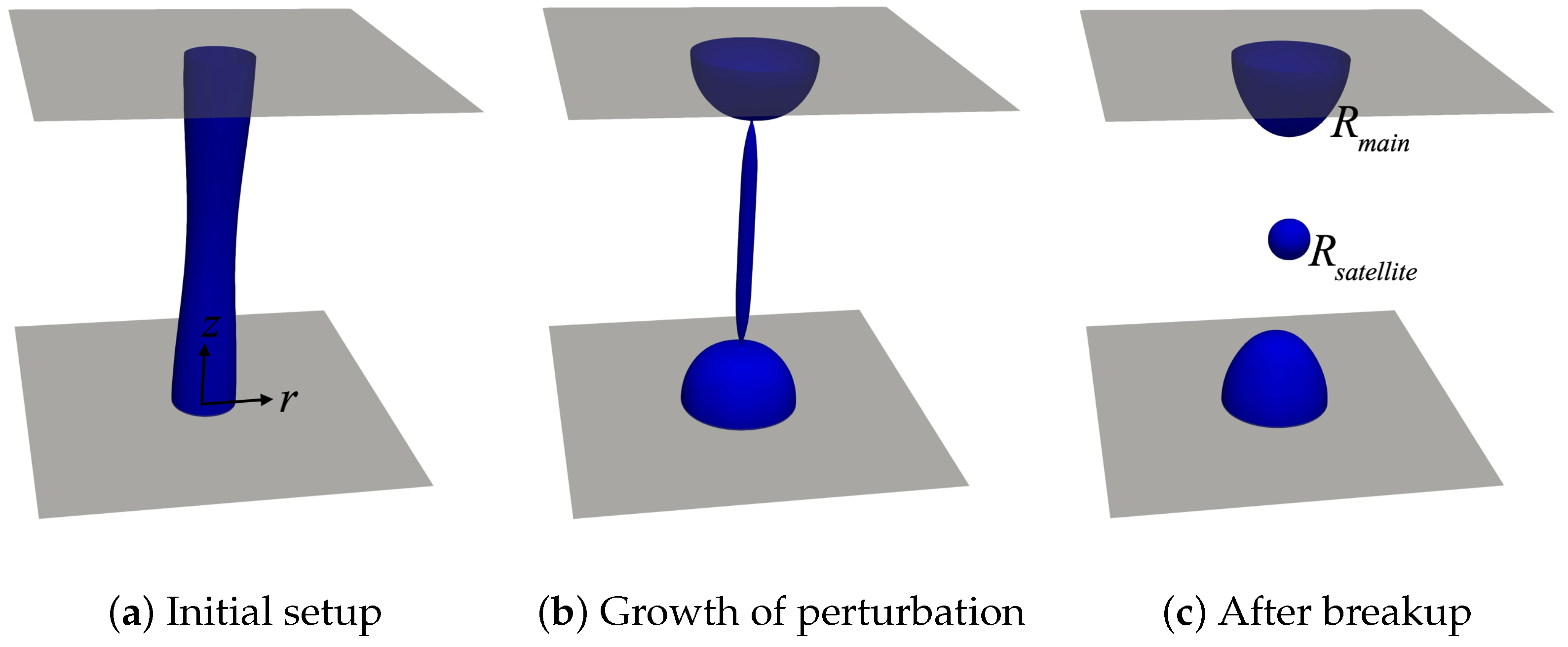
3.4. Rayleigh–Plateau Instability
Another exercise that is relevant to hydrodynamic breakup consists of a Rayleigh–Plateau instability [
30]. This is a surface tension-driven flow jet breakup under zero gravity, which is similar to ligament breakup during spray formation [
31]. The initial stage is characterized by a liquid column with a varicose sinusoidal perturbation imposed on its surface, as shown in
Figure 9a. This perturbation grows and eventually fragments the liquid column, as seen in
Figure 9b,c. The breakup leads to the formation of two structures, a large main droplet or parent droplet at the periodic boundary of the domain and a smaller satellite droplet in the central part of the domain. The periodic nature of the simulation domain in the vertical direction implies that the main droplet is continuous across the top and the bottom faces of the domain.
Lafrance [
32] provides a detailed theoretical analysis and experimental data of the breakup of the laminar liquid jet accounting for non-linear effects. We compare the present results against these theoretical predictions. All simulations are performed in a 3D domain with dimensions
, where
is the wavelength of the disturbance imposed. Periodic conditions are applied on the top and bottom boundaries. For all the other boundaries, zero gradient condition is imposed for
and velocity, and zero Dirichlet for pressure. The simulations are based on a water jet of
with
,
,
,
, and
0.073
. The spatial resolution is given by
in the region surrounding the liquid jet. Away from the jet a coarser grid is employed. The initial perturbation, which is described by the radial distance of the interface from the axis of the jet, is given by
where
and
k is the dimensionless perturbation wavenumber, given by
. Simulations with
and
are performed.
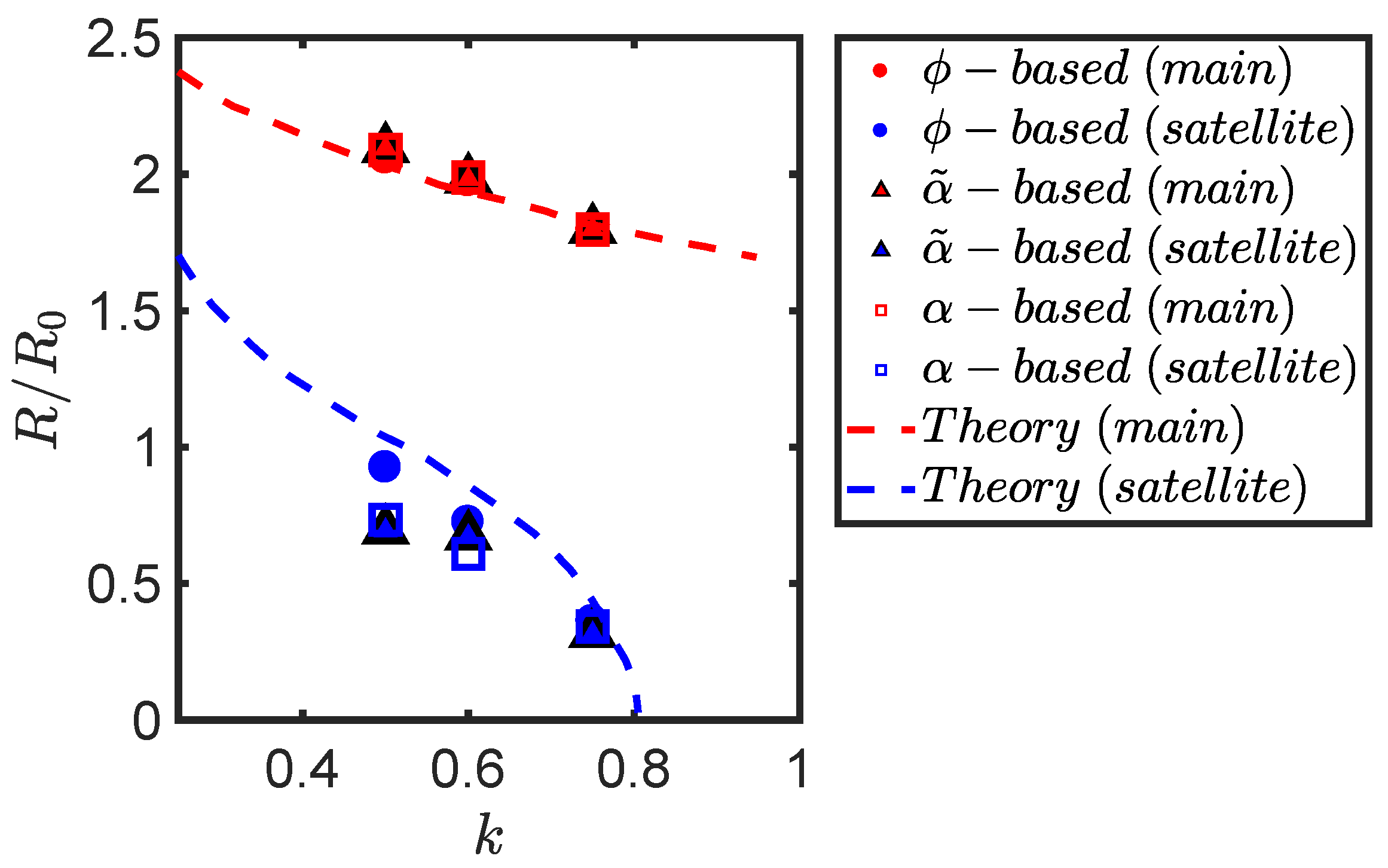
The radii of the resulting droplets are presented in
Figure 10 along with the theoretical predictions [
32]. The top and bottom curves in this plot represent, respectively, the main droplet size and satellite droplet size. The theoretical predictions are shown using dotted lines, and the simulation results are shown with different markers. Quantification of the error is provided by
where
is the numerically predicted main or satellite radii and
is the theoretical counterpart. This error data are presented in
Table 4 and
Table 5.
The main droplet size predictions corresponding to the three methods are close enough to each other that the markers in
Figure 10 practically overlap. For the satellite droplet predictions, the differences are more noticeable. This is expected since the volume of the main droplet is so much larger than the satellite droplet that numerical errors affect satellite size predictions more strongly. Among the three methods, the
-based computations lead to the best predictions consistent with previous tests; however, the results for all three methods are not drastically different. Additionally, the errors have about the same magnitude at the different wavenumbers examined. It was observed that, for some cases, the
-based method is prone to a slight departure from asymmetry, which leads to the formation of more than one satellite droplet. This raises some questions regarding the suitability of this method in breakup problems.
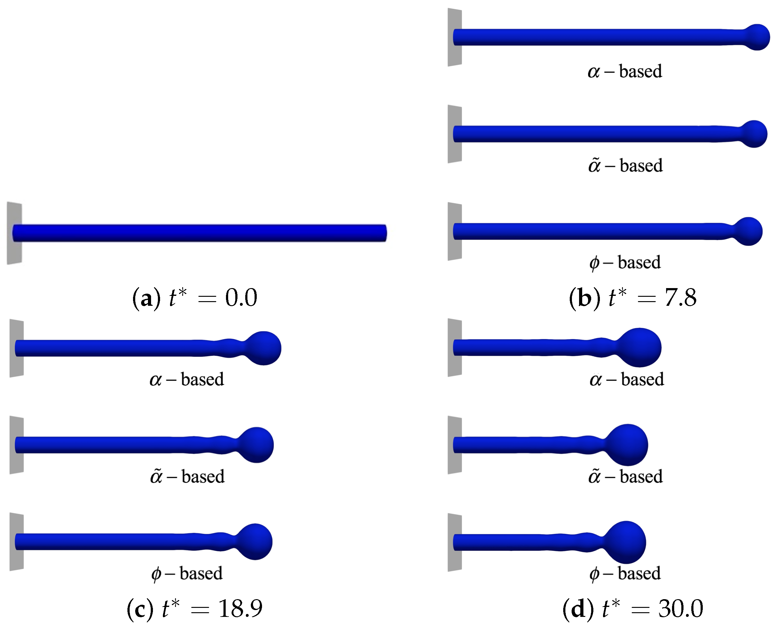
3.5. Retraction of Liquid Column
The last exercise consists of a surface tension drive retraction of a liquid column under zero gravity conditions presented by Umemura [
33]. In this last test, there are no analytical solutions and, thus, the evaluation is restricted to a comparison among the three prediction methods. The conditions employ a liquid (SF
6) with a density of
1460
, a viscosity of
, and a surface tension of
. The gas is pressurized nitrogen with a density and viscosity given, respectively, by
79.1
and
. The domain has dimensions [
mm × 0.8424 mm × 5.1168 mm] with the axis of the liquid column aligned with the
z-axis and positioned at the center of the left face. This left face is a wall, with zero gradient conditions for pressure and
, and a no-slip velocity condition. At all other boundaries, a zero gradient is applied for
and velocity, and a zero Dirichlet condition is applied for pressure. The cylindrical column has an initial radius
0.12748 mm and length 5.1168 mm.
The simulations are performed on a uniform mesh with a resolution of
μm yielding a jet diameter to grid size ratio of
32. At this level of resolution, the results for column length time history are numerically converged. Its time evolution, as shown in
Figure 11, is non-dimensionalized by the capillary time scale, which is given by
[
34] (pg. 3;) thus,
, where
R is the radius of the cylinder. In this non-dimensionalization, the wave number
has been used along with the fact that
, and thus,
can be ignored.
The perfectly cylindrical liquid column at starts retracting, and a bulb and a neck are formed at the tip, as shown on the figures at . With the persistent action of surface tension, the bulb continues to grow, as depicted at . At this middle time, subtle differences appear between prediction from the standard method and the other two methods. At the final time of = 30, the predictions between the -based and -based are essentially the same and are slightly different from the standard method.
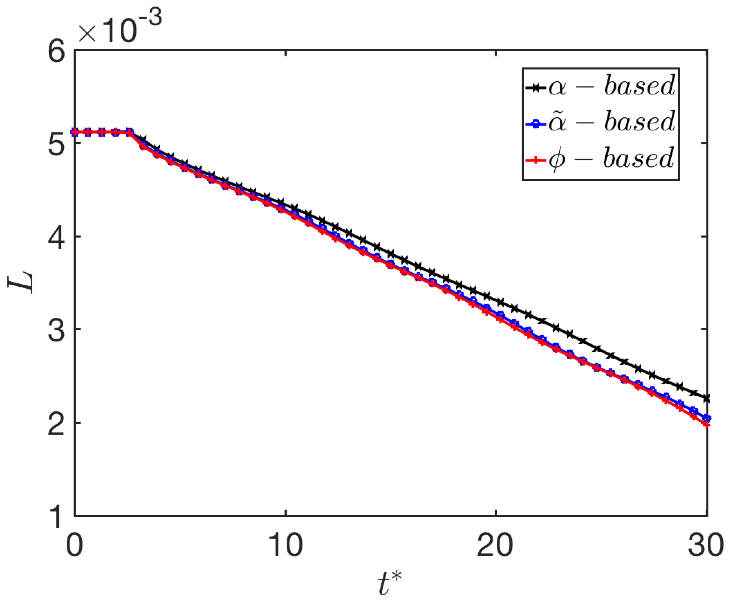
The quantitative difference among the three curvature estimation methods is provided by comparing the time history of the liquid column lengths, as shown in
Figure 12. Initially, the length of the liquid column remains unaltered as only the periphery is affected by the dynamics, but the central part remains largely unchanged. The flat predictions of column length reflect this during the initial period, which lasts until approximately
3.2. Beyond this initial period, the retraction of the liquid column is essentially a linear function of time, implying that the retraction speed is constant. The lengths from the diffused-
based method and the
-based method are almost identical and are slightly faster than the
-based computation. While subtle differences emerge in the shapes of the bulbs and the lengths of the liquid columns predicted by the three methods, the differences in the overall dynamics appear minor. An improved curvature scheme does not impact the results in a significant way.
3.6. Evaluation of Computational Costs
The calculations in the previous sections have shown that the
-based method is noticeably superior to the standard
-based calculation, particularly when the effect of surface tension is isolated from all other factors. This section documents the computational cost of exercising this
-based method, where our findings are presented in
Table 6 as a percentage of the total cost for all operations. Specifically, the
-based calculation consists of an interface reconstruction and a Hamilton–Jacobi re-initialization, as outlined in
Section 2.3. In contrast, the standard
-based method has no such interface reconstruction or re-initialization costs.
For the sake of completeness, the cost of all other operations are also included in
Table 6. This consists of the
transport operation, which consists of the solution of the VoF equation. It also includes the momentum equation, which is the predictor part of the calculation, and the Pressure–Poisson equation, which usually dominates all computational costs. Overhead costs are also included. The results show that the Pressure Poisson calculation remains, not surprisingly, the dominant contributor to the computational expense. However, the
-based operations are not necessarily negligible and, in some instances, are relatively close to the Pressure calculation. This means that, in the worst-case scenarios, the calculations involving the current
-based method can be up to 50% more expensive than the standard
-based methodology. However, it should be kept in mind that no effort has been made in expediting these additional
-based calculations at this stage. It remains part of future work.
4. Conclusions
Improvements to the interfacial curvature calculations have been implemented and tested against the standard -based methodology employed in interFoam. The new implementations consist of a diffused treatment for the liquid fraction (-based) and a signed-distance function procedure (-based). Five evaluation exercises have been performed, emphasizing hydrodynamic breakup problems, and are thus relevant to spray formation and other atomization processes.
In summary, our findings show that, among the three methods, the
-based method is consistently superior in all cases, with the most notable result being the second-order convergence of the Laplace pressure across a 2D droplet. As evident in the literature, the lack of convergence for the standard
-based method has been known for quite some time, and the
shows a lower level of error but still fails to converge. An interesting finding is that the predictions converge even for the standard method once the problem involves motion, such as the oscillating droplet case. Additionally, the predictions for the shear layer (
Section 3.3), the Rayleigh jet breakup (
Section 3.4), and the retraction of a liquid column (
Section 3.5) show that the standard method does not differ significantly from the more accurate
-based method, even though its performance is worse. The difference between
-based and
-based methods is accentuated when surface tension effects become the dominant influencing factor, for instance, for the 3D oscillating droplet.
An interesting conclusion from the present work is that, once other factors enter into the dynamics, such as viscous forces, inertia, or pressure, the performance of the standard
-based treatment becomes quite reasonable. For instance, the agreement with theory in the droplet oscillating case (
Section 3.2), the shear layer (
Section 3.3), and the Rayleigh jet (
Section 3.4) are for the most part acceptable. It is only when the evaluation exercise focuses entirely on the curvature prediction, for instance, the Laplace pressure problem (
Section 3.1) or the spurious current estimations presented in the literature [
1,
26,
35] that we see the standard method falling quite short of the exact result. However, most practical cases concerning liquid breakup do not involve such carefully orchestrated scenarios, and in these more general cases, the standard method does a reasonable job. A takeaway from the current work is that adding more complicated and accurate curvature prediction methods to
interFoam does not necessarily guarantee
meaningful improvements in realistic flow simulations unless those simulations are to a great degree governed by surface tension, e.g., nano-droplet dynamics.


