Arbitrary Hybrid Turbulence Modeling Approach for High-Fidelity NREL Phase VI Wind Turbine CFD Simulation

Abstract

Today, growth in renewable energy is increasing, and wind energy is one of the key renewable energy sources which is helping to reduce carbon emissions and build a more sustainable world. Developed countries and worldwide organizations are investing in technology and industrial application development. However, extensive experiments using wind turbines are expensive, and numerical simulations are a cheaper alternative for advanced analysis of wind turbines. The aerodynamic properties of wind turbines can be analyzed and optimized using CFD tools. Currently, there is a general lack of available high-fidelity analysis for the wind turbine design community. This study aims to fill this urgent gap. In this paper, an arbitrary hybrid turbulence model (AHTM) was implemented in the open-source code OpenFOAM and compared with the traditional URANS model using the NREL Phase VI wind turbine as a benchmark case. It was found that the AHTM model gives more accurate results than the traditional URANS model. Furthermore, the results of the VLES and URANS models can be improved by improving the mesh quality for usage of higher-order schemes and taking into consideration aeroelastic properties of the wind turbine, which will pave the way for high-fidelity concurrent multidisciplinary design optimization of wind turbines.

1. Introduction

Today, renewable energy sources play an important role in reducing CO₂ emissions, which cause global warming. Many organizations and countries are taking action to reduce CO₂ emissions and finance the development of wind energy technology. According to the Economist (2019), 7% of the total energy was received from solar panels and wind turbines in 2019, and the number is expected to increase up to fivefold by 2040 [1]. The International Energy Agency (IEA) believes and acknowledges that nuclear energy, wind energy, solar PV energy geothermal power, and hydropower will be the main power sources of the 21st century, as there is a limit on nonrenewable sources as oil, natural gas, and coal, since they last up to 30, 50, and 200 years, respectively [2]. Wind energy is the cleanest green energy available currently, and researchers are developing efficient wind turbines and testing them with wind tunnels. However, the usage of wind tunnels is expensive and time-consuming. Furthermore, scale effects cannot be properly addressed. Therefore, computational fluid dynamics (CFD) simulations are used for numerical simulations, analysis, and design optimization.

A more realistic flow through the rotors of wind turbines can be simulated using computational fluid dynamics (CFD), which numerically solves Navier–Stokes equations. On the other hand, there are other low-fidelity methods such as blade element momentum (BEM) and lifting line panel method (LLPM); however, they have some limitations when it comes to the simulation of complex three-dimensional turbulent flow, since the lifting line theory is based on potential flow theory, while the BEM is 2D momentum theory, which is highly reliant on two-dimensional airfoil data that need empirical corrections [3]. There are three main CFD approaches to simulate turbulent flows: (1) large eddy simulation (LES); (2) Reynolds-averaged Navier–Stokes (RANS); (3) the hybrid RANS–LES model (HRLM) [4,5]. The RANS model for simulation is acceptable as it can appropriately simulate steady and unsteady simulations, while the LES model is good for resolving large-scale energy containing eddies; thus, LES is more accurate than RANS but computationally much more expensive, while HRLM is more accurate than RANS and computationally cheaper than LES. Wind turbine simulation involves complex flows through its rotors, for which the RANS model currently remains the main CFD solver for HAWT aerodynamics as it is computationally cheap and generates acceptable time-averaged results. However, the HRLM will be increasingly used for complex wind turbine aerodynamic analysis and design optimization, as engineers are designing ever larger wind turbines that require multidisciplinary analysis and design, considering fluid–structure interaction, fatigue, and noise reduction, as the LES is too expensive for these tasks [6,7].

Arbitrary hybrid turbulence modeling is the arbitrary combination of the RANS turbulence method and LES in the flow field depending on the required resolution in different locations, which gives more accurate results than RANS while being cheaper than LES. By rescaling the conventional RANS equations through the introduction of the resolution control function Fr into the turbulent viscosity of the RANS turbulence model, the formulation of the new VLES model can be achieved. This resolution control factor is the ratio of sub-grid turbulent stress to the RANS/URANS turbulent stress, which can also roughly represent the ratio of modeled turbulent energy to total turbulent energy. It is responsible for smooth transitioning between RANS/URANS/LES/DNS modes depending on local mesh density in comparison with the turbulence integral and Kolmogorov length scales.

A study was performed on the mechanical responses of the National Renewable Energy Laboratory (NREL) Phase VI wind turbine using commercial application ANSYS, and the results were compared with the traditional blade element momentum (BEM) method [8]. The study found that the blade element momentum method (BEM) was not accurate, and it was also observed that applicable results could be obtained using BEM, but it was time-consuming and challenging. Furthermore, the CFD and FSI methods either overpredicted or underpredicted the power compared with experimental results.

Zhong et al. [9] performed CFD simulations using the k-omega SST model with different beta star coefficients for the NREL Phase VI wind turbine. It was found that changing the beta star value to 0.11 from 0.09 improved the results; however, the agreement between experimental values and numerical results were not satisfactory when the wind speed was 15 m/s, as the difference was more than 15%.

Another paper [10] reported a numerical study on the NREL Phase VI wind turbine using different wind speeds between 5 and 21 m/s and the Spalart–Allmaras (SA) turbulence model. The CFD computed results underpredicted the torque compared with NREL experimental data for all wind speeds. It was concluded that the differences between experimental data and CFD results were due to the limitations of the turbulence model.

Commonly, computational fluid dynamics (CFD) simulations are used to predict wind turbine performances under different wind conditions. These simulations represent numerical solutions of the Navier–Stokes equations, which describe fluid flow. Furthermore, for wind turbine CFD simulations, traditional turbulence models such as Spalart–Allmaras, k-epsilon, k-omega, and k-omega SST are used since they are as computationally effective as RANS simulations. However, engineers increasingly need to study more physical effects, such as fluid–structure interaction (FSI), fatigue, and noise for multidisciplinary design analysis and optimization (MDAO), which requires greater resolution of turbulent eddies. In order to make more accurate predictions, turbulence models such as LES, zonal detached eddy simulation (DES), or even direct numerical simulation (DNS) can be used, but they are very computationally expensive and inflexible. Therefore, in this study, we aimed to develop an arbitrary hybrid turbulence modeling (AHTM) approach based on VLES, which can help design engineers to take advantage of this unique and highly flexible approach to tailor the grid according to the design and resolution requirements in different areas of the flow field over the wind turbine without sacrificing accuracy and efficiency. This paper presents the details of the implementation and careful validation of the AHTM method using the NREL Phase VI wind turbine, in comparison with other existing models, such as RANS and URANS, showing that the VLES is the most accurate among those examined. Furthermore, the results of this study demonstrate that the AHTM approach has the flexibility, efficiency, and accuracy to be integrated with transient and concurrent MDAO tools for engineering design in the wind energy industry. Currently, the AHTM implementation is being integrated with the DAFoam for gradient-based multipoint MDAO using an efficient adjoint solver based on the sparse nonlinear optimizer (SNOPT).

2. Governing Equations and Boundary Conditions

It can be assumed that the flow is incompressible since the velocities are very small compared to the speed of sound and density does not change in the flow. The Navier–Stokes equations for mass and momentum conservation equation for three-dimensional unsteady incompressible flow are used.

$$\nabla .\mathit{u}=0.$$

(1)

$$\frac{\partial \mathit{u}}{\partial t}+\nabla .\left(\mathit{u}\mathit{u}\right)=-\frac{1}{\rho }\nabla \overline{p}+\mu \nabla .\nabla \mathit{u}+F_t.$$

(2)

In order to solve the above equations, initial and boundary conditions have to be set; thus, the domain is divided into inlet, outlet, cylinder, propeller, and Arbitrary Mesh Interface (AMI) regions.

Table 1. Boundary conditions for wind turbine simulation.

Boundary Conditions	k	nut	omega	P	U
Inlet	FixedValue	FixedValue	FixedValue	zeroGradient	FixedValue
Outlet	zeroGradient	zeroGradient	zeroGradient	FixedValue	zeroGradient
Cylinder	slip	slip	slip	slip	slip
Propeller MRF	kqRWallFunction	nutkWallFunction	omegaWallFunction	zeroGradient	fixedValue
Propeller AMI	kqRWallFunction	nutkWallFunction	omegaWallFunction	zeroGradient	movingWallVelocity
AMI1	cyclicAMI	cyclicAMI	cyclicAMI	cyclicAMI	cyclicAMI
AMI2	cyclicAMI	cyclicAMI	cyclicAMI	cyclicAMI	cyclicAMI

below presents the initial and boundary conditions for stated regions; initial values for k, nut, and omega were set to 0.375${\mathrm{m}}^2/{\mathrm{s}}^2$, ${10}^{-5}{\mathrm{m}}^2/\mathrm{s}$, and 320${\mathrm{s}}^{-1}$, respectively, according to the turbulence intensity, which was selected to be 5%. Inlet velocities were set to 7, 10, and 15 $\mathrm{m}/\mathrm{s}$.

3. Turbulence Model for RANS/URANS Simulations

There are different RANS turbulence models, e.g., one-equation, two-equation, and multi-equation models; the most popular ones are two-equation turbulence models such as k-epsilon, k-omega, and SST k-omega, which can generally produce accurate predictions for many industrial applications for certain flow conditions. The two-equation models require two transport equations to calculate turbulent viscosity. The standard k-epsilon is a widely known turbulence model that uses the turbulent kinetic energy and energy dissipation rate to calculate turbulent viscosity and thermal diffusivity. The k-omega turbulence model is a similar model to the k-epsilon model, but with different constants and replacement of epsilon by omega, which is the specific rate of turbulence dissipation representing the conversion rate of turbulence kinetic energy into internal thermal energy. Its performance is better than the k-epsilon model for predicting turbulence near walls and separated flows. The improved version of the k-omega turbulence model for resolving turbulence near the wall and flow separation is the shear stress transport (SST) k-omega model. The two equations for the SST k-omega model used in this paper are presented below [11,12,13].

The turbulence specific dissipation rate equation is:

$$\frac{D}{Dt}\left(\rho \omega \right)=\nabla ·\left(\rho D_{\omega }\nabla \omega \right)+\frac{\rho \gamma G}{v}-\frac{2}{3}\rho \gamma \omega \left(\nabla ·\mathit{u}\right)-\rho \beta {\omega }^2-\rho \left(F_1-1\right)C{D}_{k\omega }+S_{\omega }.$$

(3)

The turbulence kinetic energy equation is as follows:

$$\frac{D}{Dt}\left(\rho k\right)=\nabla ·\left(\rho D_k\nabla k\right)+\rho G-\frac{2}{3}\rho k\left(\nabla ·\mathit{u}\right)-\rho {\beta }^{\ast }\omega k+S_k.$$

(4)

The turbulence viscosity is given as:

$${\mu }_t=a_1\frac{k}{max\left(a_1\omega ,\sqrt{2}{S}_t{F}_2\right)}.$$

(5)

4. Implementation of Arbitrary Hybrid Turbulence Model

The following equation describes the general form of control function Fr, which is established from the ratio of sub-grid scale turbulence energy to the total turbulence energy:

$$F_r=\frac{{\tau }_{ij}^{VLES}}{{\tau }_{ij}^{URANS}}\approx \frac{{{\displaystyle \int }}_{L_k}^{L_c}E\left(L\right)dL}{{{\displaystyle \int }}_{L_k}^{L_i}E\left(L\right)dL}\approx \frac{\frac{\left(ln{L}_c-ln{L}_k\right)\left(ln{E}_c+ln{E}_k\right)}{2}}{\frac{\left(ln{L}_i-ln{L}_k\right)\left(ln{E}_i+ln{E}_k\right)}{2}}=\frac{\ln \left(\frac{L_c}{L_k}\right)\ln \left(E_c{E}_k\right)}{\ln \left(\frac{L_i}{L_k}\right)\ln \left(E_i{E}_k\right)},$$

(6)

where $L_c=C_{VLES}{({\mathsf{\Delta }}_x{\mathsf{\Delta }}_y{\mathsf{\Delta }}_z)}^{1/3}$ is the cutoff length scale, $L_i=\frac{k^{3/2}}{\epsilon }$ is the integral length scale, and $L_k=\frac{v^{3/4}}{{\epsilon }^{1/4}}$ is the Kolmogorov length scale. Moreover, ${\mathsf{\Delta }}_x, {\mathsf{\Delta }}_y, \mathrm{and} {\mathsf{\Delta }}_z$ are the mesh dimensions in different directions, and the laminar kinematic viscosity is υ. According to Equation (6), the resolution control function represents the ratio of the unresolved turbulence energy to the total turbulent energy [14]. It was subsequently modified to the following form, which adopts the minimum value between 1.0 and the modified Speziale model [15]:

$$F_r=min\left(1.0,{\left[\left(1.0-exp\left(-\beta L_c/L_k\right)\right)/\left(1.0-exp\left(-\beta L_i/L_k\right)\right)\right]}^n\right),$$

(7)

$$L_c=C_x{\left({\mathsf{\Delta }}_z{\mathsf{\Delta }}_y{\mathsf{\Delta }}_z\right)}^{1/3}; L_i=\frac{k^{\frac{3}{2}}}{\epsilon }; L_k=\frac{{\nu }^{\frac{3}{4}}}{{\epsilon }^{\frac{1}{4}}},$$

where L_c, L_i, and L_k are the turbulent cutoff length scale, integral length scale, and Kolmogorov length scale, respectively, ${\mathsf{\Delta }}_x,{\mathsf{\Delta }}_y$, and ${\mathsf{\Delta }}_z$ are mesh scales in different directions, and $\nu$ is the laminar viscosity. Recommended values for $n$ and $\beta$ are n $=\frac{4}{3}$, $n=2$, and $\beta =2.0\times {10}^{-3}$ according to the study of Speziale et. al. [16]. The model constant $C_x$ can be calibrated using $C_{\mu }=0.09$, which is the model constant of the turbulence model (in this case, SST k-omega model), and $C_s=0.1$, which is the typical Smagorinsky LES model constant [8]. Thus, $C_x=\sqrt{0.3}{C}_s/C_{\mu }=0.61$. This resolution control function can be used to dampen the turbulent viscosity of the k-omega SST turbulence model as ${\mu }_t=F_r{v}_t$, where ${\mu }_t$ is the new turbulent viscosity, $F_r$ is the resolution control function, and $v_t$ is the turbulent viscosity of the turbulence model [17].

As discussed before, the VLES formulation can give better results than RANS/URANS models and is cheaper than LES; thus, the model was implemented into OpenFOAM through the modification of the k-omega shear stress transport (kOmegaSST) model since this turbulence model gives more accurate results than other turbulence models for wind turbine simulation. First, applying all the recommended values and model constants into the resolution control function, the following expression could be derived for the resolution control function:

$$F_r=\min (1.0,{\left[\frac{\left(1.0-\exp (-\beta {\frac{L_c}{L}}_k \right)}{\left(1.0-\exp (-\frac{\beta L_i}{L_k}\right)}\right]}^{\frac{4}{3}}).$$

(8)

$$F_r=\min (1.0,{\left[\frac{\left(1.0-\exp \left( \beta C_x{({\mathsf{\Delta }}_x{\mathsf{\Delta }}_y{\mathsf{\Delta }}_z)}^{\frac{1}{3}}\frac{{(C_{\mu }k\omega )}^{\frac{1}{4}} }{{\nu }^{\frac{3}{4}}}\right)\right)}{\left(1.0-\exp \left(-\frac{\beta }{{\left(C_{\mu }\right)}^{\frac{3}{4}}}{\left(\frac{k}{\nu \omega }\right)}^{\frac{3}{4}}\right)\right)}\right]}^{\frac{4}{3}}).$$

(9)

Furthermore, the kOmegaSST turbulence model equations proposed by Menter et al. [16] were the same as given in Equations (3)–(5), and the turbulence viscosity term of the model was modified as follows for VLES implementation:

$${\mu }_t=F_r{a}_1\frac{k}{max\left(a_1\omega ,\sqrt{2}{S}_t{F}_2\right)}.$$

(10)

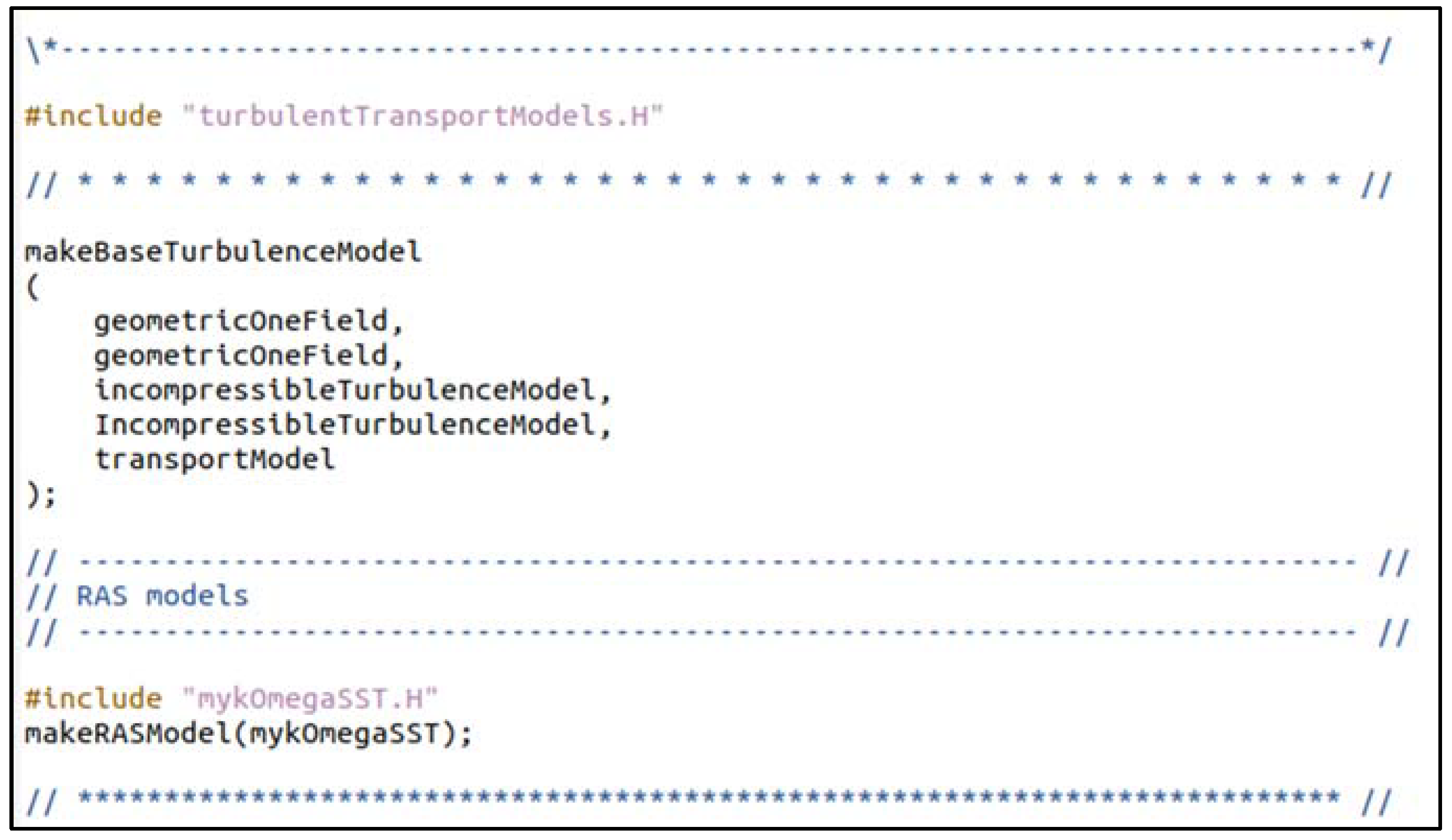
Now, the VLES was implemented into the OpenFOAM with source codes in the directory mykOmegaSST, and a library was created from mykOmegaSST and other OpenFOAM directories. First, the makeTurbulenceTransportmodels.C file was modified as shown in Figure 1.

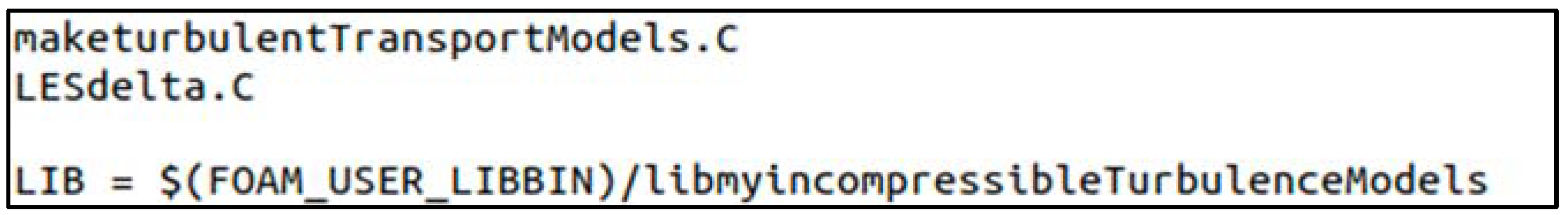
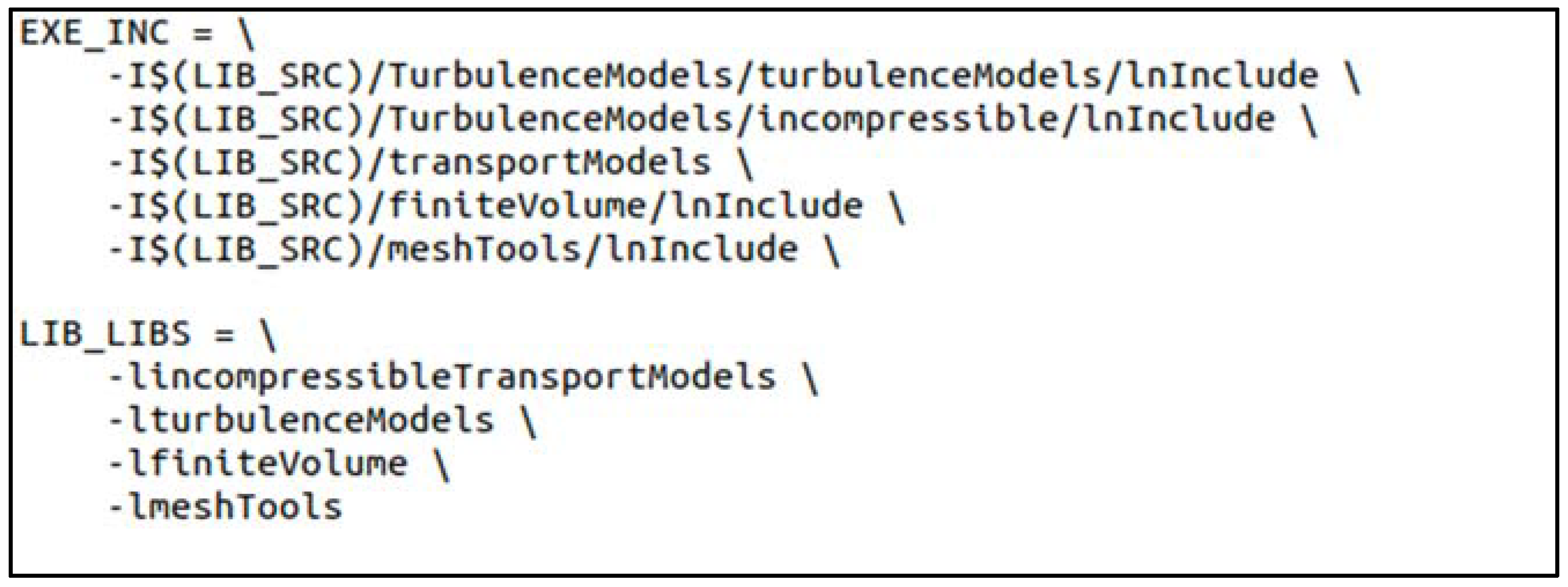
Then, a folder with the name Make was created in the mykOmegaSST directory, and the files and options source codes were created as shown in Figure 2 and Figure 3, respectively.

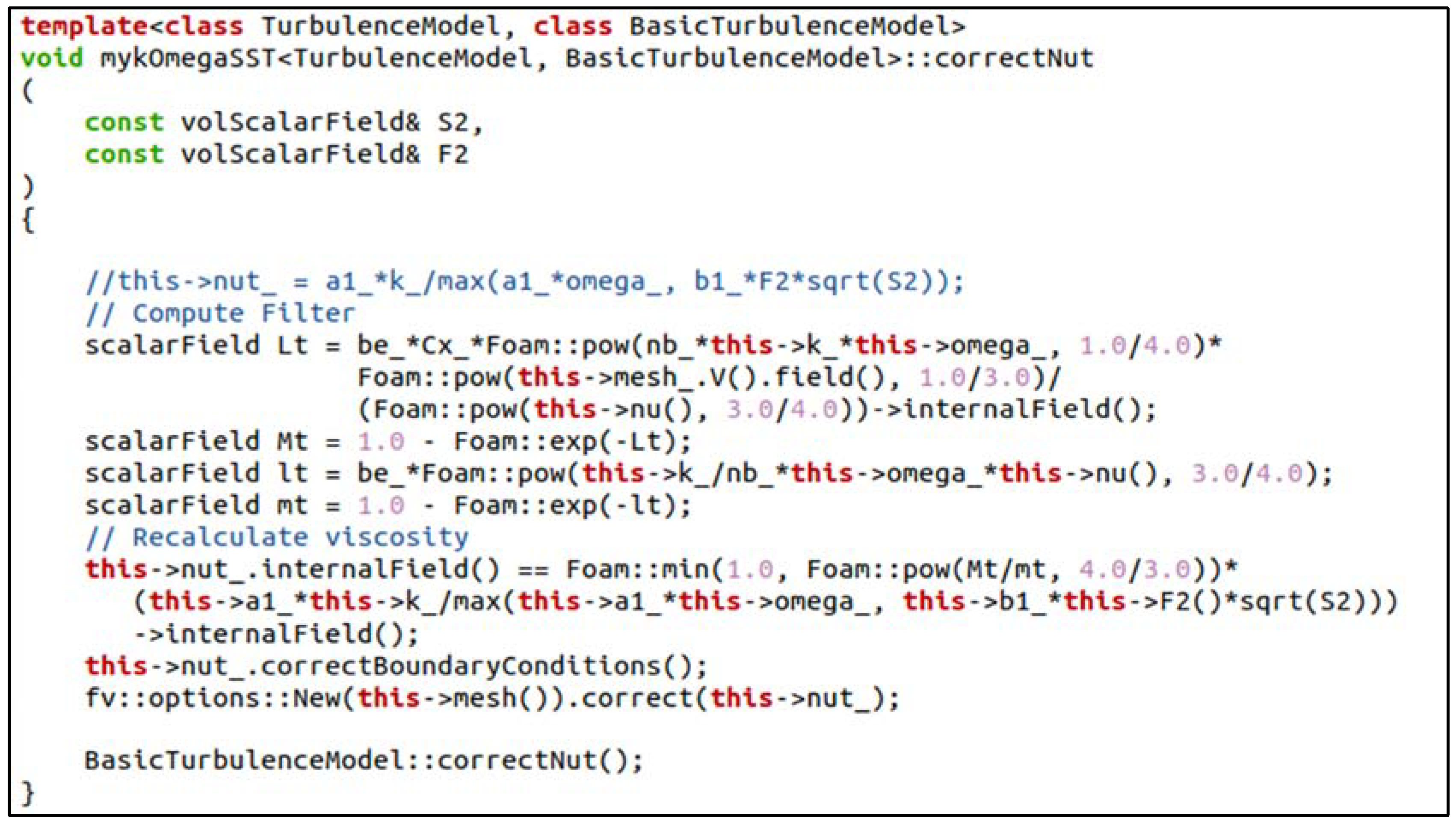
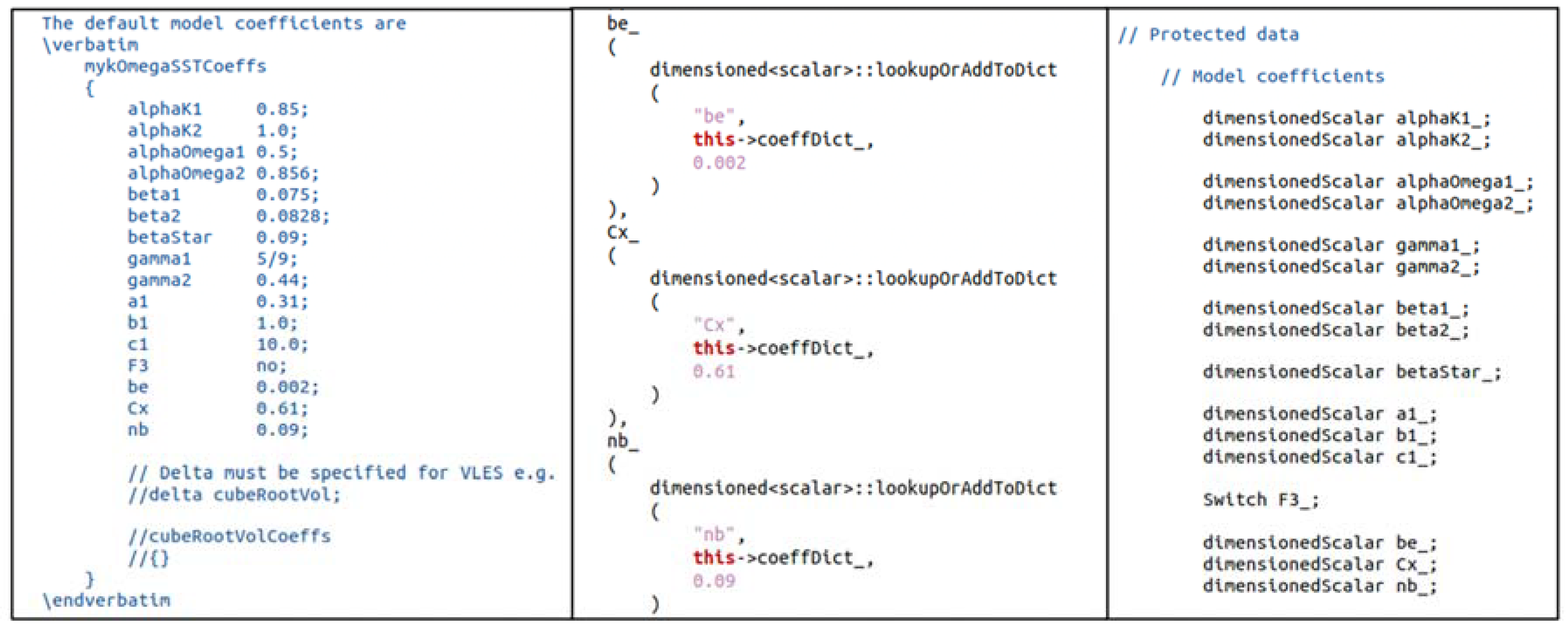
After that, the kOmegaSST files and base files were copied from OpenFOAM to the mykOmegaSST directory, and the modified version of the kOmegaSST or VLES is shown in Figure 4.

The code shown above is the resolution control function added to the turbulence viscosity of the kOmegaSST. In addition, the recommended values and model constants need to be added as shown in Figure 5.

Once, all the necessary files were modified and created, the codes were compiled and a library was created via the wmake libso command. Furthermore, to run the VLES model for any simulation, the controlDict and turbulenceProperties files need to be changed. Links for all the necessary files to compile the model are included in Appendix A.

5. Results and Discussion

5.1. Mesh Generation and Mesh Convergence Study

The geometry of the NREL Phase VI wind turbine was created according to Figure 6 by SolidWorks, together with the cylindrical outer domain and the cylindrical domain for the AMI zone. The dimensions of the outer domain were as follows: (1) diameter = 100 m and length = 150 m; (2) diameter and length of the MRF/AMI domain = 20 m and 26 m, respectively.

Creating a high-quality mesh is one of the most important and hardest procedures in CFD in order to obtain correct and accurate results. Many applications can be used for mesh generation, and one of them is snappyHexMesh, which generates dominant hexahedral meshes using existing simple meshes generated by blockMesh. However, this mesh generation tool cannot be used for the NREL Phase VI wind turbine since it cannot create good boundary layers. Therefore, another mesh generator called Pointwise was used for generating meshes over the NREL Phase VI wind turbine since it creates structural hyperbolic boundary layers for the wind turbine. Furthermore, a combination of structural and unistructural approaches was applied, i.e., a hybrid mesh was used for mesh creation except for the boundary layers of around the turbine blades. Figure 7, Figure 8, Figure 9 and Figure 10 show examples of the generated meshes.

A mesh convergence study aims to determine the most appropriate mesh for further simulation by increasing mesh density to the extent that there are no significant changes in the computational results with optimal mesh density for accuracy and, at the same time, high computational efficiency. Therefore, the inlet wind speed was set to 15 m/s, and the rotational velocity of the wind turbine was set to 72 rpm. The k-omega SST VLES turbulence model was used for simulation, and the case was run for 1 s. The initial mesh had about 17 million cells, which was then increased up to around 55 million cells until the relative error between the CFD and experimental results was reduced to less than 5% as shown in

Table 2. Mesh convergence study.

Type	Mesh #1	Mesh #2	Mesh #3	Mesh #4
Number of cells	17,131,110	24,078,878	36,932,383	54,937,248
Average torque value (N·m)	582.3	634.5	668.3	680.5
Experimental torque	710.0
Difference in values (%)	18.0	10.6	5.9	4.2

.

5.2. URANS and VLES Results

In this section, the CFD simulation results of the NREL Phase VI are described and compared with experimental data for validation. Hand et al. tested the NREL Phase VI wind turbine in the wind tunnel and provided the data used in this article for comparison with numerical results. The NREL Phase VI wind turbine was tested using different cone angles, blade tip pitches, and other parameters and for each specific case of ordinal number. In this paper, experimental data with ordinal number I was used [12]. Since the mesh size was relatively large, only three different speeds were used. Figure 11 shows the pressure coefficients of the URANS and VLES numerical simulations compared with experimental data at different spans. Simulations were performed until the time reached 1.2 s and wind speed was 7 m/s. It can be seen from Figure 11 that URANS and VLES pressure coefficients were the same as the experimental data except for the leading edge, where a higher pressure difference occurred.

Table 3. Comparison of CFD torque values with experimental data (wind speed = 7 m/s).

Type	VLES (Average)	URANS (Average)	Experiment
Average torque (N·m)	823.6	926.1	834.2
Error to experiment (%)	1.3	11.0	-

and

Table 4. Comparison of CFD power values with experimental data (wind speed = 7 m/s).

Type	Transient VLES (Average)	URANS (Average)	Experiment
Average power (kW)	6.21	6.98	6.28
Error to experiment (%)	1.1	11.1	-

below show the difference between numerical results and experimental data, with the VLES simulation results giving more accurate values than URANS.

Overall, at a wind speed of 7 m/s, VLES results were better than those of URANS. In addition, it can be seen from Figure 12 that VLES could capture and resolve more eddies on the surface of the wind turbine than URANS judging from the vorticity contours shown.

In Figure 13, pressure coefficients and the corresponding experimental data for different sections of the NREL Phase VI wind turbine according to VLES and URANS simulations are presented for a wind speed of 10 m/s. As can be seen from Figure 13, numerical pressure coefficient results agreed well with the experimental measurements.

Table 5. Comparison of CFD torque values with experimental data (wind speed = 10 m/s).

Type	VLES (Average)	URANS (Average)	Experiment
Average torque (N·m)	880.0	1141.8	980.5
Error to experiment (%)	10.2	16.5	-

and

Table 6. Comparison of CFD power values with experimental data (wind speed 10 = m/s).

Type	Transient VLES (Average)	URANS (Average)	Experiment
Average power (kW)	6.64	8.61	7.39
Error to experiment (%)	10.1	16.5	-

show a comparison of the numerical and experimental torque and power results, with the VLES model performing better than URANS; however, both turbulence models had more than 10% error. One of the reasons might be blade deformation. The maximum output of the NREL Phase VI wind turbine is reached when the wind speed was 10 m/s.

Figure 14 shows the vorticity contours for a wind speed of 10 m/s. Compared with Figure 12 for a wind speed of 7 m/s, the flow field had much more smaller eddies as the wind speed was higher. Similarly, the arbitrary hybrid turbulence model could better capture/resolve turbulence eddies than the URANS model. Moreover, URANS and VLES vortex results were compared using the Lambda2 criterion to detect vortices (according to Jeong et al., it can identify vortex core geometry correctly from a three-dimensional fluid velocity field [18]). Thus, Figure 15 shows a comparison between URANS and VLES results using the Lambda2 criterion.

Figure 16 shows the pressure coefficients of the URANS and VLES numerical simulations and their comparison with experimental data for a wind speed of 15 m/s. Simulations were performed until the time reached 1.2 s. It can be seen that numerical pressure coefficients agreed well with the experimental data.

Table 7. Comparison of CFD torque values with experimental data (wind speed = 15 m/s).

Type	VLES (Average)	URANS (Average)	Experiment
Average torque (N·m)	680.5	660.2	710.0
Error to experiment (%)	4.2	7.0	-

and

Table 8. Comparison of CFD power values with experimental data (wind speed = 15 m/s)

Type	Transient VLES (Average)	URANS (Average)	Experiment
Average power (kW)	5.35	5.13	5.34
Error to experiment (%)	0.2	3.9	-

present the torque and power values, respectively, for transient simulations compared with the experimental result, where it can be observed that VLES results ere better compared with URANS.

Figure 17 shows the vorticity contours for a wind speed of 15 m/s, where the helical vorticity contours at the tip were destroyed due to the high wind speed and flow instability, compared with the vorticities at lower wind speed.

5.3. High-Accuracy VLES Results

It can be seen from Table 5 and Table 6 that the torque and power values of URANS and VLES results had more than 10% error compared to experimental data when the wind speed was 10 m/s. Therefore, a hybrid upwind scheme called the LUST (with 75% linear and 25% linear upwind) was employed to generate more accurate results. However, this was unsuccessful for URANS since the solution became unstable and the simulation crashed after around 0.03 s. For VLES, it worked but the computational time was increased substantially, taking around 9 days to complete 0.1 s of simulation. Therefore, the computational simulation was run only for 0.1 s. The average torque and power values for VLES were around 1026.5 N·m and 7.74 kW, i.e., only 4.7% and 2.3% difference, respectively, compared with experimental data. In addition, in Figure 18, vorticity contours of the NREL Phase VI wind turbine are shown with the new results. Comparing the results in Figure 14 and Figure 18, it can be seen that using the LUST scheme with VLES could capture and resolve more eddies near the wind turbine. Furthermore, the work can be improved further by simulating the wind turbine using LES and comparing the results among the three different models, although it was found by our group in previous work [19,20] that the LES results are comparable to RANS/URANS in terms of accuracy.

6. Parallel Computation

Today, high-performance computers (HPCs) are effective ways to simulate large numerical models in parallel using a greater number of processors than traditional computers. However, the speed of the simulations is not increased with the number of processors; for this analysis, 16 processors were used for parallel computation. Due to the number of models that needed to be simulated, two different HPCs are used.

Table 9. Characteristics of the HPCs.

Overview	HPC 1	HPC 2
Processor	Intel® Xeon(R) Gold 5118CPU (Intel Corporation, Santa Clara, California and U.S.)@ 2.30 GHz	Intel® Xeon(R) CPU E5-2699 v4 @ 2.20 GHz
Number of processors	48	88
Memory	251.5 GB	503.8 GB
Operating System (OS)	Ubuntu

shows the overview of the HPCs.

Thus, the computational time of the simulations is shown in

Table 10. Comparison of the CPU times used by URANS and VLES simulations.

CPU Time	Wind Speed = 7 m/s	Wind Speed = 10 m/s	Wind Speed = 15 m/s
VLES	31.4 days	39.6 days	42.2 days
URANS	24.0 days	27.8 days	29.3 days

for a simulation time of 0.8 s. It can be seen from Table 10 that URANS was computationally more effective than VLES; however, HPC 2 which was used for the URANS simulations was faster than HPC 1 which was used for the VLES simulations.

7. Conclusions

In this work, an arbitrary hybrid turbulence modeling approach for wind turbine aerodynamic analysis was developed and implemented in OpenFOAM using the VLES model for the purpose of highly efficient concurrent and transient multidisciplinary design optimization (MDO) by the wind energy engineering community for the design of future wind turbines. Transient CFD simulations were conducted to analyze the NREL Phase VI wind turbine for different wind speeds with the VLES and URANS turbulence models implemented. All simulations were performed using OpenFOAM except for mesh creation. It was found that the VLES model gave better results than URANS for all the tested wind speeds compared to experimental data. For wind speeds of 7 m/s and 15 m/s, the differences between experimental and numerical torque and power values were smaller than 5% for VLES, whereas, for URANS, the differences were more than 5% for both parameters except for numerical power at a wind speed of 15 m/s, which had less than 5% error compared to experimental power. However, for a wind speed of 10 m/s, the difference between numerical and experimental data was relatively high, but it could be improved by considering FSI. Numerical VLES results were improved using a higher-order divergence scheme, but this did not work for URANS. Thus, the error between numerical and experimental torque and power values was reduced from 10.2% to 4.7% and from 10.1% to 2.3% respectively. The most accurate result was achieved using the VLES model for a wind speed of 7 m/s.

References

1. Supplying Clean Power Is Easier than Storing It. The Economist. 29 November 2019. Available online: https://www.economist.com/business/2019/11/28/supplying-clean-power-is-easier-than-storing-it (accessed on 3 February 2020).
2. IEA. World Energy Outlook 2019; IEA: Paris, France; Available online: https://www.iea.org/reports/world-energy-outlook-2019 (accessed on 15 March 2022).
3. Li, Y.; Paik, K.-J.; Xing, T.; Carrica, P.M. Dynamic overset CFD simulations of wind turbine aerodynamics. Renew. Energy 2012, 37, 285–298. [Google Scholar] [CrossRef]
4. Yu, H.; Thé, J. Simulation of gaseous pollutant dispersion around an isolated building using the k–ω SST (shear stress transport) turbulence model. J. Air Waste Manag. Assoc. 2017, 67, 517–536. [Google Scholar] [CrossRef] [PubMed] [Green Version]
5. Yu, H.; Thé, J. Validation and optimization of SST k-ω turbulence model for pollutant dispersion within a building array. Atmos. Environ. 2016, 145, 225–238. [Google Scholar] [CrossRef]
6. Yang, Z. Large-eddy simulation: Past, present and the future. Chin. J. Aeronaut. 2015, 28, 11–24. [Google Scholar] [CrossRef] [Green Version]
7. Baker, C.; Johnson, T.; Flynn, D.; Hemida, H.; Quinn, A.; Soper, D.; Sterling, M. Computational techniques. Train Aerodyn. 2019, 53–71. Available online: https://www.sciencedirect.com/science/article/pii/B9780128133101000046 (accessed on 15 March 2022). [CrossRef]
8. Lee, K.; Huque, Z.; Kommalapati, R.; Han, S.-E. Fluid-structure interaction analysis of NREL phase VI wind turbine: Aerodynamic force evaluation and structural analysis using FSI analysis. Renew. Energy 2017, 113, 512–531. [Google Scholar] [CrossRef]
9. Zhong, W.; Tang, H.; Wang, T.; Zhu, C. Accurate RANS Simulation of Wind Turbine Stall by Turbulence Coefficient Calibration. Appl. Sci. 2018, 8, 1444. [Google Scholar] [CrossRef] [Green Version]
10. Song, Y.; Perot, J. CFD simulation of the NREL phase VI rotor. Wind. Eng. 2014, 39, 299–310. [Google Scholar] [CrossRef] [Green Version]
11. Moukalled, F.; Mangani, L.; Darwish, M. The Finite Volume Method in Computational Fluid Dynamics; Springer: Cham, Switzerland, 2016. [Google Scholar]
12. Hand, M.; Simms, D.; Fingersch, L.J.; Jager, D.; Larwood, S.; Cotrell, J.; Schreck, S. Unsteady Aerodynamics Experiment Phase VI: Wind Tunnel Test Configurations and Available Data Campaigns; NREL/TP-500-29955; National Renewable Energy Laboratory (NREL): Golden, CO, USA, 2001. [Google Scholar]
13. Jasni, N.A.H.; Lajis, M.A. A comprehensive study on surface roughness in machining of AISI D2 hardened steel. Adv. Mater. Res. 2012, 576, 60–63. [Google Scholar] [CrossRef]
14. Han, X.; Krajnović, S. A New Very Large Eddy Simulation Model for Simulation of Turbulent Flow. In Progress in Hybrid RANS-LES Modelling; Fu, S., Haase, W., Peng, S.H., Schwamborn, D., Eds.; Notes on Numerical Fluid Mechanics and Multidisciplinary Design; Springer: Berlin/Heidelberg, Germany, 2012; Volume 117. [Google Scholar] [CrossRef] [Green Version]
15. Spalart, P.R. Detached-eddy simulation. Annu. Rev. Fluid Mech. 2009, 41, 181–202. [Google Scholar] [CrossRef]
16. Speziale, C.G. Turbulent modeling for time-dependent RANS and VLES: A review. AIAA J. 1998, 36, 173–184. [Google Scholar] [CrossRef]
17. Menter, F.R.; Kuntz, M.; Langtry, R. Ten years of industrial experience with the SST turbulence model. In Proceedings of the Fourth International Symposium on Turbulence, Heat and Mass Transfer, Antalya, Turkey, 12–17 October 2003; Begell House: Redding, CT, USA; pp. 625–632. [Google Scholar]
18. Jeong, J.; Hussain, F. On the identification of a vortex. J. Fluid Mech. 1995, 285, 69–94. [Google Scholar] [CrossRef]
19. Igali, D.; Mukhmetov, O.; Zhao, Y.; Fok, S.C.; Teh, S.L. Comparative Analysis of Turbulence Models for Automotive Aerodynamic Simulation and Design. Int. J. Automot. Technol. 2019, 20, 1145–1152. [Google Scholar] [CrossRef]
20. Sadykov, S.; Khalimov, R.; Kylyshbek, Y.; Batay, S.; Kaishubayeva, N.; Zhao, Y.; Fok, S.C.; Teh, S.L. An URANS simulation of the kelvin-helmholtz aerodynamic effect over the ahmed body. Int. J. Automot. Sci. Technol. 2021, 5, 166–171. [Google Scholar] [CrossRef]
Figure 1. The makeTurbulenceTransportmodels.C file.
Fluids 07 00236 g001
Figure 2. The files source code.
Fluids 07 00236 g002
Figure 3. The options source code.
Fluids 07 00236 g003
Figure 4. The modified turbulence viscosity for VLES.
Fluids 07 00236 g004
Figure 5. The recommended values and model constants.
Fluids 07 00236 g005
Figure 6. NREL Phase VI wind turbine blade dimensions [12].
Fluids 07 00236 g006
Figure 7. Full domain for the CFD simulation (view: cut in half).
Fluids 07 00236 g007
Figure 8. AMI (rotating) zone of the wind turbine.
Fluids 07 00236 g008
Figure 9. Hyperbolic boundary layers of the NREL Phase VI wind turbine (top view).
Fluids 07 00236 g009
Figure 10. Hyperbolic boundary layers of the NREL Phase VI wind turbine (side view).
Fluids 07 00236 g010
Figure 11. Pressure coefficients for URANS, VLES, and experiment (wind speed = 7 m/s).
Fluids 07 00236 g011
Figure 12. Vorticity contours when wind speed = 7 m/s and time = 1.2 s (left: VLES; right: URANS).
Fluids 07 00236 g012
Figure 13. Pressure coefficients of URANS, VLES, and experiment (wind speed = 10 m/s).
Fluids 07 00236 g013
Figure 14. Vorticity contours when wind speed = 10 m/s and time = 1.4 s (left: VLES; right: URANS).
Fluids 07 00236 g014
Figure 15. Lambda2 criterion when wind speed = 10 m/s and time = 1.4 s (left: VLES; right: URANS).
Fluids 07 00236 g015
Figure 16. Pressure coefficients of URANS, transient VLES, and experiment (wind speed = 15 m/s).
Fluids 07 00236 g016
Figure 17. Vorticity contours when wind speed = 15 m/s and time = 1.2 s (left: VLES; right: URANS).
Fluids 07 00236 g017
Figure 18. Vorticity contours when wind speed = 10 m/s (VLES).
Fluids 07 00236 g018