Estimation of Flow Field in Natural Convection with Density Stratification by Local Ensemble Transform Kalman Filter

Abstract

For estimating thermal flow in a nuclear reactor during an accident accurately, it is important to improve the accuracy of computational fluid dynamics simulations. The temperature and flow velocity are not homogeneous and have large variations in a reactor containment vessel because of its very large volume. In addition, Kelm’s work pointed out that the influence of variations of initial and boundary conditions was important. Therefore, it is necessary to set the initial and boundary conditions taking into account the variations of these physical quantities. However, it is a difficult subject to set such complicated initial and boundary conditions. Then, we can obtain realistic initial and boundary conditions and an accurate flow field by data assimilation, and we can improve the accuracy of the simulation result. In this study, we applied data assimilation by a local ensemble transform Kalman filter to a simulation of natural convection behavior in density stratification, and we performed a twin model experiment. We succeeded in estimating the flow fields and improving the simulation accuracy by the data assimilation, even if we applied the boundary condition with error for the true condition.

1. Introduction

During a severe accident, hydrogen gas is generated by a water–zirconium reaction in a nuclear reactor core, and there is a risk of a hydrogen explosion in a containment vessel (CV) of a nuclear reactor. A hydrogen explosion is one of the most important phenomena in safety evaluation. A CV has a complex geometry and a very large volume. So, hydrogen can be distributed locally, and multidimensional flow is dominant in a CV. The temperature and velocity distributions are not homogeneous. Therefore, it is important to evaluate the gas behavior in a CV accurately and to improve the accuracy of computational fluid dynamics (CFD) simulation for the safety evaluation of the thermal–hydraulic behavior.

Kelm et al. pointed out that the influence of variations of initial and boundary conditions is important and the use of accurate initial and boundary conditions is required for an accurate numerical simulation of the behavior inside a CV [1]. In addition, we revealed that the temperature boundary condition of a small internal structure in a CV has a large influence on the fluid temperature distribution [2]. Therefore, it is necessary to set the initial and boundary conditions taking into account the variations of these physical quantities. However, it is a difficult subject to set such complicated initial and boundary conditions.

Here, we focus on data assimilation to obtain accurate initial and boundary conditions, which has been applied recently in various fields. Data assimilation is a method to reduce the errors of numerical simulation and to obtain more realistic simulation results and simulation parameters by referring to observation data. Several studies applying data assimilation to thermal flow simulations were reported. Cornick et al. applied a local ensemble transform Kalman filter (LETKF) to flows in Rayleigh-Bénard convection experiments, and they estimated the flow state and the model parameter [3]. Decker et al. compared a simplified model of natural convection similar to the Lorentz system with a CFD simulation of a thermosyphon to test a data assimilation method and understand the convection dynamics. Flow reversals were successfully forecast in the related Lorenz model [4]. Reagan et al. performed a twin model experiment with a CFD simulation of thermal convection in a loop using an ensemble transform Kalman filter (ETKF) to predict flow reversals. They showed that using adaptively shaped localized covariance outperformed static localized covariance with the ETKF [5]. Introini et al. applied a Kalman filter to Reynolds averaged Navier–Stokes (RANS) equations for turbulent flow, and they extended the integration of the Kalman filter to a thermodynamic simulation of turbulent flow [6]. The proposed method by Introini et al. ensures mass conservation. The accuracy of the algorithm was verified for a heated lid-driven cavity flow.

However, the study about the data assimilation for the thermal–hydraulic simulation in a CV has not been carried out sufficiently, and its performance and applicability have not been clarified. In this article, we focus on the natural convection behavior induced by the external cooling of a vessel as a benchmark problem. This behavior is important for the evaluation of the thermal–hydraulic behavior in a CV during a severe accident, and an accurate simulation of this behavior is necessary for the safety evaluation. We simulate the natural convection behavior in a small vessel scaled down from the large-scale containment vessel facility CIGMA (Containment Integral effects Measurement Apparatus) [7] considering the similarity. The detail of the problem definition is described in the next section. Then, the data assimilation is applied to the simulation of the natural convection in this small vessel, and this data assimilation test is conducted as a first step to investigate the efficiency of the data assimilation for the simulation of thermal–hydraulic behavior in a CV. In this study, we use the LETKF [8] as the data assimilation method. We investigate the influence of observation locations, physical quantities to be observed and objects of the data assimilation. We conduct the sensitivity evaluations.

2. Problem Definition

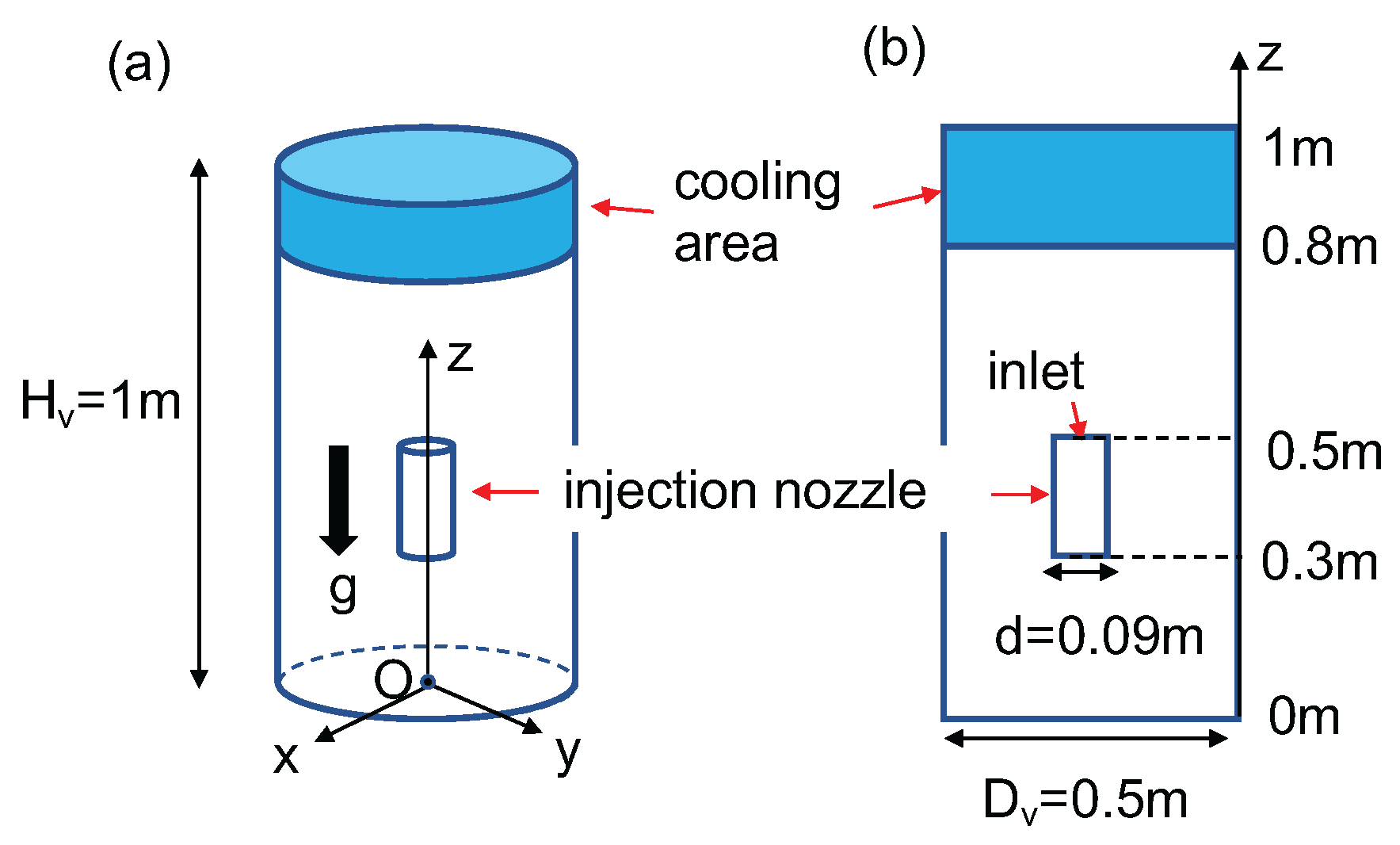
2.1. Natural Convection with Density Stratification

We conducted an experiment on the natural convection behavior with the density stratification using the CIGMA facility in the previous study [7]. In this experiment, the density stratification was built up initially in the vessel by injection of the mixture of air and helium (a simulant of hydrogen). After the termination of the gas injection, the outside vessel wall was cooled. The natural convection was induced by this external cooling. The problem definition of this study was determined by referring to this CIGMA experiment. We simulated the natural convection with the density stratification in the small vessel scaled down from the CIGMA facility because the CIGMA facility is a large system and it takes a long time to simulate the flow behavior in the CIGMA facility.

Figure 1 shows schematic views of the vessel. We considered a closed cylindrical vessel. The diameter of the vessel $D_v$ and the height $H_v$ were 0.5 m and 1 m, respectively. The coordinate origin is located at the center of the vessel’s bottom. The z direction corresponds to the vertical direction. Initially, the vessel was filled with air of 153 kPa and 400 K, and a quiescent state ($(u_1,u_2,u_3)=(0,0,0)$, where $u_1,u_2,u_3$ are the velocity components in the $x,y,z$ directions) was maintained at 0 s (step 1). Helium gas was injected from the inlet of the injection nozzle shown in Figure 1 for 0–10 s (step 2). The start time (0 s) was set as the initiation time of the helium injection. We built up a density stratification layer. After the termination of the helium gas injection, the quiescent state was maintained for 10–15 s (step 3). The pressure at 15 s was about 175 kPa. After that, the external cooling of the upper region of the vessel $z=$ 0.8–1 m was initiated and maintained for 15–100 s (step 4). During the external cooling, the wall temperature of the cooling area was maintained at 300 K (${T|}_w=$ 300 K, where ${T|}_w$ is the temperature on the wall), and the other wall temperatures were 400 K (${T|}_w=$ 400 K). Then, the natural convection was induced in the vessel. The detailed simulation procedure is described in Section 2.2. We estimated the flow field after the initiation of the external cooling by the data assimilation.

The interaction between convective flow and density stratification is characterized by the interaction Froude number [9]. The interaction Froude number is defined as $Fr=\frac{U}{N{D}_v}$, where $N=\sqrt{\frac{2g({\rho }_0-{\rho }_s)}{({\rho }_0+{\rho }_s)H_s}}$ is the characteristic strength of density stratification [10] and $U=\sqrt{\frac{2g{D}_v({\rho }_s-{\rho }_w)}{{\rho }_s+{\rho }_w}}$ is the buoyancy velocity scale [11]. g is the gravity acceleration. ${\rho }_0,{\rho }_s,{\rho }_w$ are the air density, the mixture gas density in stratification, and the mixture gas density near the cooled wall, respectively. $H_s$ is the height of the gradient layer of the stratification. The Froude number was adjusted to a value similar to that of the CIGMA experiment, that is, $Fr=0.73$ of the CC-PL-27 experiment in the literature [7]. We set the Froude number $Fr=0.73$ in this simulation.

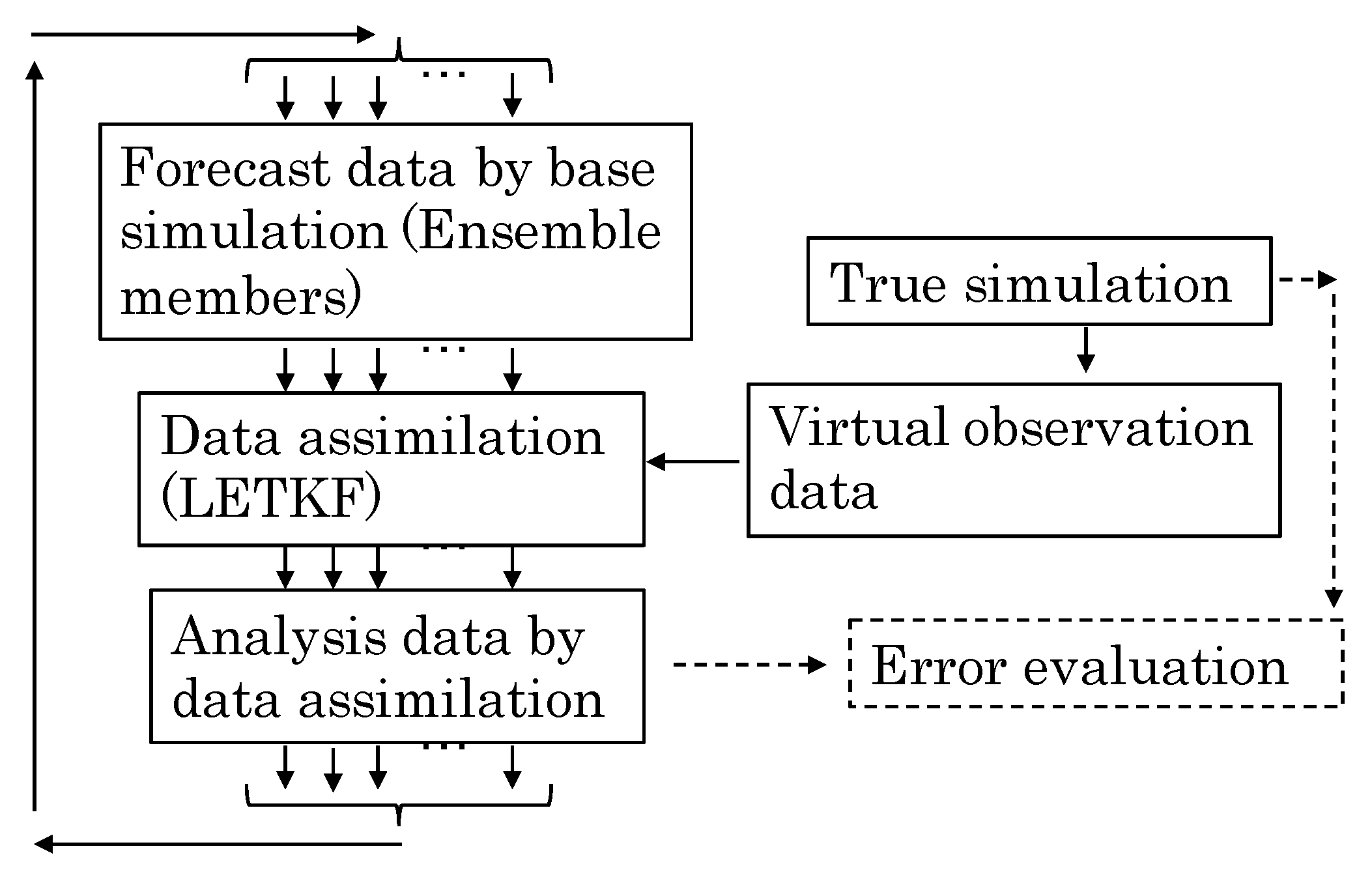
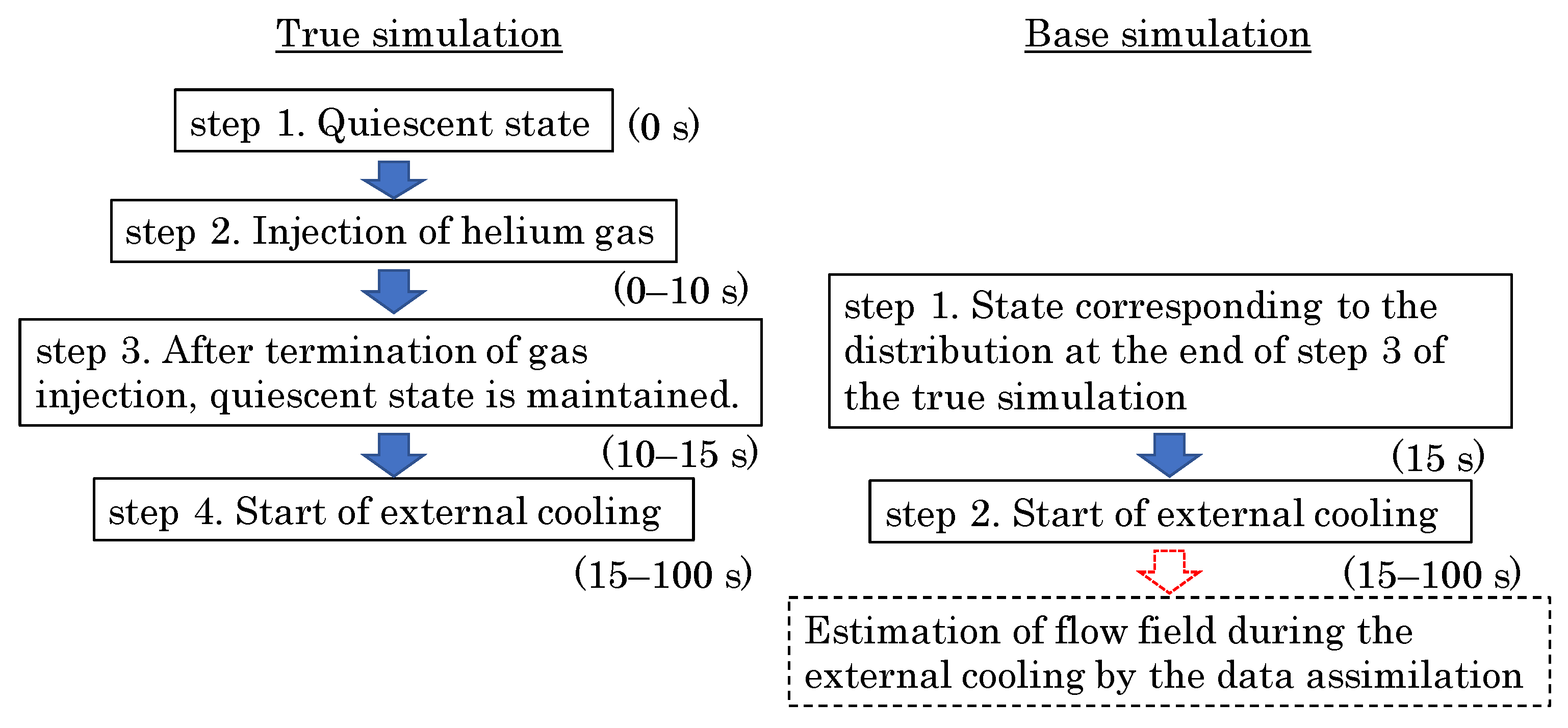
2.2. Twin Model Experiment and Simulation Procedures

We conducted a twin model experiment instead of the analysis using actual experimental data. A flow chart of the twin model experiment is shown in Figure 2. In the twin model experiment, we performed a true simulation which gave a true solution and a base simulation to which the different initial and boundary conditions from the true simulation were applied. We obtained forecast data by the base simulation and analysis data by applying the data assimilation to the forecast data. Hereafter, the analysis data refer to the values obtained by data assimilation. We applied the LETKF as the data assimilation in this study. So, it was necessary to generate multiple ensemble members, and we generated the ensemble members by the data of the base simulation. The algorithm of the LETKF is described in Section 4.1. We used virtual observation data generated by adding noise to the true simulation data instead of the experimental observation data. By using the true simulation data and the analysis data, we evaluated the errors of the analysis results. We investigated the improvement in accuracy between the forecast data and the analysis data through the data assimilation, and we discussed the performance of the data assimilation.

We show the procedures of the true and base simulations for the twin model experiment described above. The simulation flow charts are shown in Figure 3. We simulated the natural convection behavior from step 1 to step 4. This is the procedure of the true simulation. The initial condition of the base simulation was the state corresponding to the distribution at the end of step 3 of the true simulation (at 15 s). The detail of the initial state of the base simulation is described in Section 3.3. The start time of the base simulation was set to 15 s. The boundary and initial conditions of the true simulation and the base simulation during the external cooling are summarized in

Table 1. Boundary and initial conditions of the true and base simulations.

	Boundary Condition	Initial Condition at The Initiation of Cooling (15 s)
True simulation	Wall temperature condition BC 1 cooling area: ${T|}_w=$ 300 K injection nozzle: ${T|}_w=$ 400 K other: ${T|}_w=$ 400 K	Quiescent state after the helium injection
Base simulation	Wall temperature condition BC 2 cooling area: ${T|}_w=$ 303 K injection nozzle: adiabatic condition (${\partial T/\partial n|}_w=0$) other: ${T|}_w=$ 404 K	Quiescent state corresponding to the end of step 3 of the true simulation

. For the base simulation, we applied the temperature boundary condition with one percent error for the temperature of the true simulation. The temperature conditions of the vessel wall in the cooling area and the other area were 303 K (${T|}_w=$ 303 K) and 404 K (${T|}_w=$ 404 K) for the base simulation, respectively. On the injection nozzle wall, we assumed the adiabatic condition (${\partial T/\partial n|}_w=0$, where n is the normal unit vector to the wall) in the base simulation. We describe the temperature boundary condition of the true simulation as condition BC 1 and that of the base simulation as condition BC 2. For the true and base simulations, non-slip condition ($(u_1,u_2,u_3)=(0,0,0)$) and zero gradient conditions of the pressure and the gas mass fraction ($\partial p/\partial n=0$ and $\partial Y/\partial n=0$, where p and Y are the pressure and the gas mass fractions of air or helium) were applied on the wall.

3. Numerical Simulation Method

3.1. Governing Equations

The numerical simulation method of fluid behavior was the same as in our previous study [2]. The numerical solver has been validated by using the results of the natural convection experiment [2] and the density stratification breakup experiment by a jet [12]. The governing equations are the mass, momentum, energy equations, and transport equations for the gas species [13]. In this simulation, we treated all gas species as ideal gas. The equation of state of the ideal gas was also applied. The gas consisted of helium and air. Helium, nitrogen, and oxygen are not involved in heat transfer by thermal radiation. Because carbon dioxide in the air is minimal, we ignored the effect of the thermal radiation. We simulated the natural convection behavior with the density stratification of air and helium ignoring the thermal radiation [2], and we obtained valid results. The RANS model was used, and the Reynolds-averaged equations are shown in Equations (1)–(4). Operators $\overline{x}$ and $\tilde{x}$ mean Reynolds averaged quantity and mass-weighted averaged (Favre averaged) quantity ($\tilde{x}=\overline{\rho x}/\overline{\rho }$), respectively.

$$\begin{array}{cc}\hfill & \frac{\partial \overline{\rho }}{\partial t}+\frac{\partial }{\partial x_i}\left(\overline{\rho }\widetilde{u_i}\right)=0\hfill \end{array}$$

(1)

$$\begin{array}{cc}\hfill & \frac{\partial }{\partial t}\left(\overline{\rho }\widetilde{u_i}\right)+\frac{\partial }{\partial x_j}\left(\overline{\rho }\widetilde{u_i}\widetilde{u_j}\right)=-\frac{\partial \overline{p}}{\partial x_i}+\frac{\partial }{\partial x_j}\left\{(\mu +{\mu }_t)\left(\frac{\partial \widetilde{u_i}}{\partial x_j}+\frac{\partial \widetilde{u_j}}{\partial x_i}-\frac{2}{3}\frac{\partial \widetilde{u_k}}{\partial x_k}{\delta }_{ij}\right)-\frac{2}{3}\overline{\rho }k{\delta }_{ij}\right\}+\overline{\rho }{g}_i\hfill \end{array}$$

(2)

$$\begin{array}{cc}\hfill & \frac{\partial }{\partial t}\left(\overline{\rho }\tilde{h}\right)+\frac{\partial }{\partial x_i}\left(\overline{\rho }\widetilde{u_i}\tilde{h}\right)=\frac{\partial }{\partial x_i}\left[\overline{\rho }\left\{(\alpha +{\alpha }_t)\frac{\partial \tilde{h}}{\partial x_i}+(D+D_t-\alpha -{\alpha }_t)\sum _n{\tilde{h}}_n\frac{\partial {\tilde{Y}}_n}{\partial x_i}\right\}\right]+\frac{\partial \overline{p}}{\partial t}\hfill \end{array}$$

(3)

$$\begin{array}{cc}\hfill & \frac{\partial }{\partial t}\left(\overline{\rho }{\tilde{Y}}_n\right)+\frac{\partial }{\partial x_i}\left(\overline{\rho }\widetilde{u_i}{\tilde{Y}}_n\right)=\frac{\partial }{\partial x_i}\left\{\overline{\rho }(D+D_t)\frac{\partial {\tilde{Y}}_n}{\partial x_i}\right\}\hfill \end{array}$$

(4)

where $\rho$, $u_i$, p, h, and $Y_n$ are density, velocity component in the i direction, pressure, enthalpy, and mass fraction of gas specie n (air or helium), respectively. $h_n$ is the enthalpy of the gas species n. $g_i$ is the gravity acceleration component in the i direction. $\mu$ is molecular viscosity, and $\alpha (=\lambda /\rho C_p)$ and D are molecular diffusivities of the enthalpy and the mass fraction. $\lambda$ and $C_p$ are molecular heat conductivity and isobaric specific heat. ${\mu }_t,{\alpha }_t,D_t$ are turbulent viscosity and turbulent diffusivity of the enthalpy and the mass fraction. $D_t$ is expressed as $D_t={\mu }_t/\overline{\rho }S{c}_t$, where $S{c}_t$ is the turbulent Schmidt number.

The standard k–$\epsilon$ model with a buoyancy effect [14] was applied with a wall function. Transport equations for turbulent kinetic energy k and the turbulent energy dissipation rate $\epsilon$ are shown in Equations (5) and (6).

$$\begin{array}{cc}\hfill & \frac{\partial }{\partial t}\left(\overline{\rho }k\right)+\frac{\partial }{\partial x_i}\left(\overline{\rho }\widetilde{u_i}k\right)=P_k+G_k-\overline{\rho }\epsilon +\frac{\partial }{\partial x_i}\left\{\left(\mu +\frac{{\mu }_t}{{\sigma }_k}\right)\frac{\partial k}{\partial x_i}\right\}\hfill \end{array}$$

(5)

$$\begin{array}{cc}\hfill & \frac{\partial }{\partial t}\left(\overline{\rho }\epsilon \right)+\frac{\partial }{\partial x_i}\left(\overline{\rho }\widetilde{u_i}\epsilon \right)=\left\{C_{\epsilon 1}(P_k+C_{\epsilon 3}{G}_k)-C_{\epsilon 2}\overline{\rho }\epsilon \right\}\frac{\epsilon }{k}+\frac{\partial }{\partial x_i}\left\{\left(\mu +\frac{{\mu }_t}{{\sigma }_{\epsilon }}\right)\frac{\partial \epsilon }{\partial x_i}\right\}\hfill \end{array}$$

(6)

Production terms $P_k$ and $G_k$ are modeled by Equation (7). The turbulent viscosity ${\mu }_t$ is expressed as ${\mu }_t=\overline{\rho }{C}_{\mu }\frac{k^2}{\epsilon }$.

$$\begin{array}{c}\hfill P_k=\left\{{\mu }_t\left(\frac{\partial \widetilde{u_i}}{\partial x_j}+\frac{\partial \widetilde{u_j}}{\partial x_i}-\frac{2}{3}\frac{\partial \widetilde{u_k}}{\partial x_k}{\delta }_{ij}\right)-\frac{2}{3}\overline{\rho }k{\delta }_{ij}\right\}\frac{\partial \widetilde{u_i}}{\partial x_j},G_k=-{\displaystyle \frac{{\mu }_t}{S{c}_t}}\frac{g}{\overline{\rho }}{\displaystyle \frac{\partial \overline{\rho }}{\partial z}}\end{array}$$

(7)

The model parameters are $C_{\mu }=0.09,{\sigma }_k=1.0,{\sigma }_{\epsilon }=1.3,C_{\epsilon 1}=1.44,C_{\epsilon 2}=1.92$, and $C_{\epsilon 3}=1$ ($G_k>0$) or 0 ($G_k\le 0$) [15].

In this study, the evaluation of the gas concentration distribution is important. In the previous study [16], we investigated the performance of the dynamic Schmidt number model, and we revealed that the simulation using this model could simulate the gas concentration behavior more accurately than the simulation using the constant Schmidt number model. We simulated the impinging jet into the density stratification using the standard k–$\epsilon$ model with the dynamic Schmidt number model [12], and we obtained valid simulation results. We applied the standard k–$\epsilon$ model with the dynamic Schmidt number model, the same as in the previous study [12]. The formulation of $S{c}_t$ is described as Equation (8). This formulation is based on the literature [17].

$$\begin{array}{c}\hfill S{c}_t=S{c}_{t0}exp\left(-{\displaystyle \frac{R{i}_g}{S{c}_{t0}{C}_1}}\right)+{\displaystyle \frac{R{i}_g}{C_2}},\end{array}$$

(8)

where $S{c}_{t0}$ is the turbulent Schmidt number under the condition of $R{i}_g=0$. $R{i}_g$ is the gradient Richardson number defined by N and the mean shear flow rate $S=\sqrt{\frac{1}{2}{\left(\frac{\partial \widetilde{u_i}}{\partial x_j}+\frac{\partial \widetilde{u_j}}{\partial x_i}\right)}^2}$ ($R{i}_g=N^2/S^2$). Here, $C_1=1/3,C_2=1/4,S{c}_{t0}=1$. The turbulent Prandtl number $P{r}_t$(=${\mu }_t/\overline{\rho }{\alpha }_t)$ was assumed to be equal to $S{c}_t$, namely ${\alpha }_t=D_t$.

3.2. Simulation Method

In this simulation, we applied the PIMPLE scheme as the pressure–velocity coupling. The PIMPLE scheme is the combination of the SIMPLE scheme [18] and the PISO scheme [19]. The governing equations were discretized by the finite volume method. An open-source CFD code OpenFOAM was used for the simulation. The version of the OpenFOAM was 2.3.x [20]. We controlled the time increment so that the maximum Courant number was 0.3. The convergence criterion for the pressure was the residual <${10}^{-8}$, and those of the other quantities were the residual <${10}^{-7}$. In the previous study, we investigated the influence of the mesh non-orthogonality on the buoyant flows [21]. Then, we applied the non-orthogonal correction to reduce the influence of the mesh non-orthogonality [22].

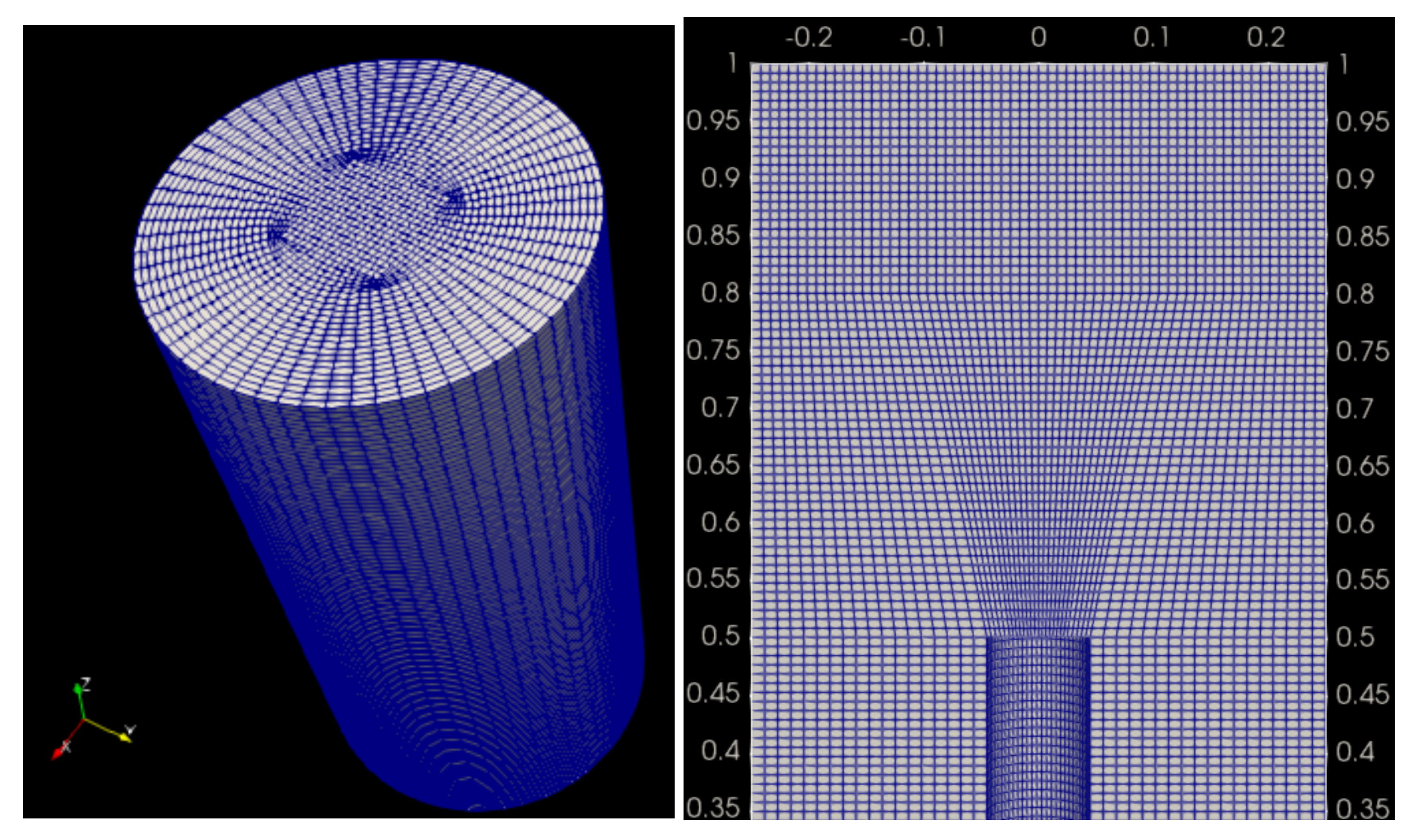
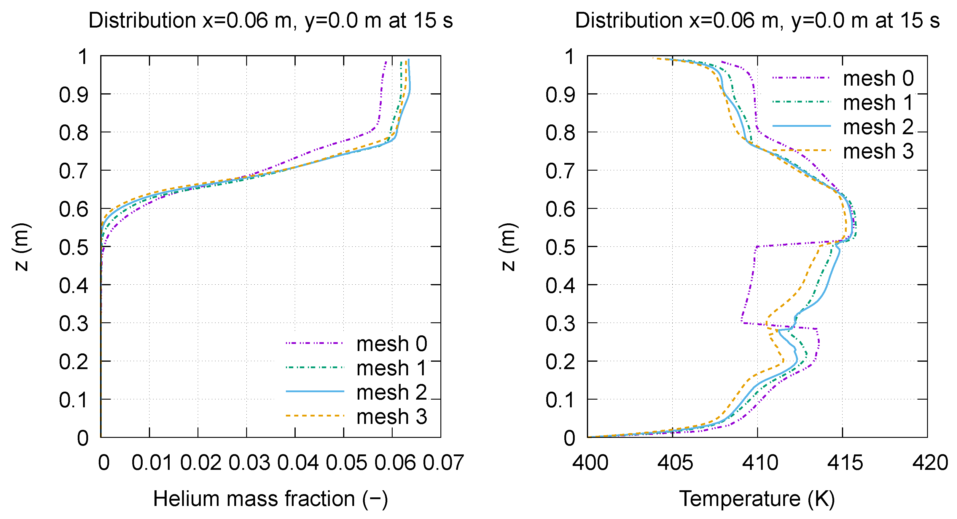
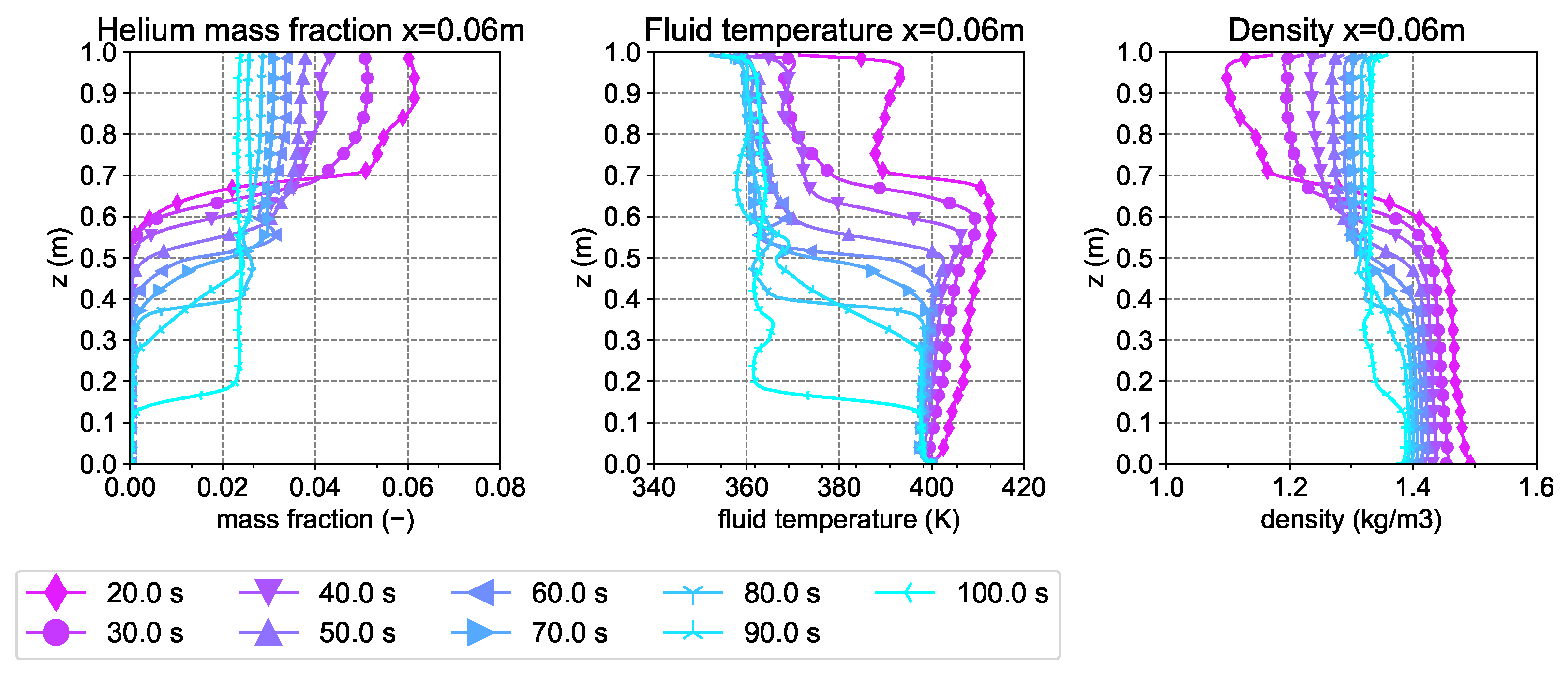
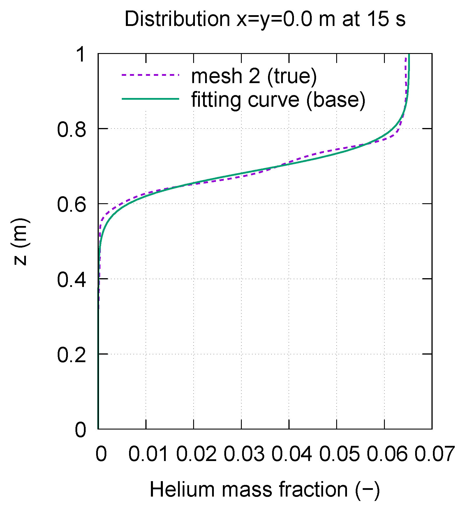
3.3. Mesh Sensitivity, True Simulation Results, and Initial Distributions of Base Simulation

We made four meshes with different mesh resolutions, and we investigated the influence of the mesh resolution. Representative mesh sizes and mesh resolutions (the total mesh numbers) are summarized in

Table 2. Representative mesh sizes and mesh resolutions.

	Representative Mesh Size	Total Mesh Number
Mesh 0	15.6 mm	26,592
Mesh 1	10 mm	109,200
Mesh 2	8 mm	203,328
Mesh 3	6.4 mm	397,040

. Figure 4 shows the overhead and cross-section views of mesh 2. The numerical meshes were composed of hexahedral elements. The mesh size near the upper and lower surface of the injection nozzle was smaller than that of the other region. The vertical distributions of the helium mass fraction and the temperature of the true simulation along $x=0.06$ m and $y=0.0$ m at 15 s are shown in Figure 5. The distributions are shown just before cooling. The results using meshes 1, 2, and 3 are almost identical and do not differ significantly. So, meshes 1–3 have sufficient mesh resolution. Hereafter, we show the results using mesh 2. Non-dimensional length $y^{+}$ at the neighbor cell of the wall was evaluated on the upper region of the vessel. The maximum values of $y^{+}$ were about 35 at 10 s and about 23 at 100 s. These values of $y^{+}$ were almost reasonable.

Time histories of the vertical distributions of the helium mass fraction, temperature, and density are shown in Figure 6 by the true simulation, and these distributions are along $x=0.06$ m and $y=0.0$ m. The external cooling was initiated at 15 s, and the distributions during the cooling are shown. Through the external cooling of the top region, the natural convection in the upper region was enhanced, and the gas mixing progressed. Then, the helium-rich layer in the upper region expanded downward. In addition, the low-temperature region expanded downward, and the density difference between the upper region and the lower region decreased. These results are qualitatively reasonable behaviors compared with the CIGMA experiment result [7].

The initial gas distribution of the base simulation was determined by fitting a hyperbolic tangent function to the gas distribution of the true simulation result at 15 s. The mass fraction of the helium $Y_{He}$ was determined by the equation $Y_{He}\left(z\right)=0.03275+0.032599tanh\left(12.797(z-0.6871)\right).$ Figure 7 shows the distributions of the helium mass fraction of the base and true simulations along the center axis ($x=y=0.0$ m) at 15 s. The distributions of the base and true simulations are indicated by solid and dashed lines, respectively. We assumed the initial temperature distribution (the temperature distribution at 15 s) of the base simulation was homogeneous, and the initial temperature was 410 K. The initial velocity distribution of the base simulation was $(u_1,u_2,u_3)=(0,0,0)$. In the base simulation, these distributions were used as the initial gas distribution.

4. Data Assimilation by Local Ensemble Transform Kalman Filter (LETKF)

In this article, the local ensemble transform Kalman filter (LETKF) was applied. The algorithm of the LETKF and the procedure of the data assimilation are described in this section.

4.1. Algorithm of LETKF

The LETKF is one of the sequential data assimilation methods. We describe the algorithm of the LETKF based on the literature [8]. We perform the data assimilation by using m ensemble members in a local patch, which is a partial region in the simulation domain. We consider an N-dimensional system state vector ${\mathit{x}}_t$ at the time step t in a local patch. The size of N is equal to the product of the number of cells in a local patch and the number of analysis variables (the physical quantities). We apply the system model M to the analysis ensemble members ${\mathit{x}}_{t-1}^{a\left(i\right)}$ ($i=1,\dots ,m$) at the time step $t-1$, where M represents the Navier–Stokes Equations (1)–(4). We obtain the forecast ensemble members ${\mathit{x}}_t^{f\left(i\right)}$ at the time step t.

$$\begin{array}{c}\hfill {\mathit{x}}_t^{f\left(i\right)}=M\left({\mathit{x}}_{t-1}^{a\left(i\right)}\right)(i=1,\dots ,m)\end{array}$$

(9)

where the superscripts $f,a$ indicate the forecast and analysis values. Equation (9) represents the forecasts of m state vectors. The forecast mean vector $\overline{{\mathit{x}}^f}$ and the forecast error covariance matrix $P^f$ for ${\mathit{x}}^{\mathbf{f}\left(\mathbf{i}\right)}$ are defined as

$$\begin{array}{cc}\hfill \overline{{\mathit{x}}^f}& =\frac{1}{m}\sum _i{\mathit{x}}^{f\left(i\right)}\hfill \end{array}$$

(10)

$$\begin{array}{cc}\hfill P^f& =\frac{1}{m-1}\delta X^f\delta X^{fT}\hfill \end{array}$$

(11)

where the columns of $\delta X^f$ are the forecast ensemble perturbation ${\mathit{x}}^{f\left(i\right)}-\overline{{\mathit{x}}^f}$, namely, $\delta X^f=[{\mathit{x}}^{f\left(1\right)}-\overline{{\mathit{x}}^f},\dots ,{\mathit{x}}^{f\left(m\right)}-\overline{{\mathit{x}}^f}]$. The subscript about the time step t is omitted. The superscript T represents the transposed matrix. We use the relationship $\delta X^a=\delta X^{f}T$, where T is the transformation matrix. We obtain Equation (12).

$$\begin{array}{cc}\hfill P^a& =\frac{1}{m-1}\delta X^a\delta X^{aT}=\frac{1}{m-1}\delta X^{f}T{T}^T\delta X^{fT}\hfill \\ \hfill & =\delta X^f\widetilde{P^a}\delta X^{fT}\hfill \end{array}$$

(12)

where $\widetilde{P^a}$ is the analysis error covariance matrix $\widetilde{P^a}=T{T}^T/(m-1)$. The size of $\widetilde{P^a}$ is $m\times m$. We obtain $T=\sqrt{m-1}{\left(\widetilde{P^a}\right)}^{1/2}$. From the relationship between $P^a$ and $P^f$, $P^a=(I-KH)P^f$, we obtain the following equation.

$$\begin{array}{cc}\hfill P^a& =\delta X^f{[(m-1)I+\delta Y^T{R}^{-1}\delta Y]}^{-1}\delta X^{fT}\hfill \end{array}$$

(13)

where K is the Kalman gain $K=\delta X^f\delta Y^T{(\delta Y\delta Y^T+(m-1)R)}^{-1}$. H is the observation matrix, and R is the observation error covariance matrix. I is the identity matrix with the size $m\times m$. $\delta Y$ is defined as $\delta Y=H\delta X^f$. So, we obtain Equation (14).

$$\begin{array}{c}\hfill \widetilde{P^a}={[(m-1)I+\delta Y^T{R}^{-1}\delta Y]}^{-1}\end{array}$$

(14)

We apply the eigenvalue decomposition as below.

$$\begin{array}{c}\hfill (m-1)I+\delta Y^T{R}^{-1}\delta Y=UD{U}^T\end{array}$$

(15)

where $U,D$ are the eigenvectors and the eigenvalues, respectively. We obtain the equation of $\delta X^a$ as Equation (16) from Equations (14) and (15).

$$\begin{array}{cc}\hfill \delta X^a& =\delta X^{f}T=\delta X^f\sqrt{m-1}{\widetilde{P^a}}^{1/2}=\delta X^f\sqrt{m-1}U{D}^{-1/2}{U}^T\hfill \end{array}$$

(16)

The analysis mean vector $\overline{{\mathit{x}}^a}$ is obtained as Equation (17) by using $K=\delta X^f\delta Y^T{(\delta Y\delta Y^T+(m-1)R)}^{-1}=\delta X^f{[(m-1)I+\delta Y^T{R}^{-1}\delta Y]}^{-1}\delta Y^T{R}^{-1}$.

$$\begin{array}{cc}\hfill \overline{{\mathit{x}}^a}& =\overline{{\mathit{x}}^f}+K(\mathbf{y}-H\overline{{\mathit{x}}^f})=\overline{{\mathit{x}}^f}+\delta X^f\widetilde{P^a}\delta Y^T{R}^{-1}(\mathbf{y}-H\overline{{\mathit{x}}^f})\hfill \end{array}$$

(17)

where $\mathbf{y}$ is the observed data vector with the size $p\times 1$. From the above, we obtain the LETKF analysis Equation (18).

$$\begin{array}{cc}\hfill X^a& =\overline{X^a}+\delta X^a=\overline{X^f}+\delta X^f[\widetilde{P^a}\delta Y^T{R}^{-1}(Y-H\overline{X^f})+\sqrt{m-1}U{D}^{-1/2}{U}^T]\hfill \end{array}$$

(18)

where the columns of $X^a$, $\overline{X^a}$ and Y are the analysis vector, the analysis mean vector, and the observed data vector. $X^a=[{\mathit{x}}^{a\left(1\right)},\dots ,{\mathit{x}}^{a\left(m\right)}]$, $\overline{X^a}=[\overline{{\mathit{x}}^a},\dots ,\overline{{\mathit{x}}^a}]$ and $Y=[\mathbf{y},\dots ,\mathbf{y}]$. The sizes of $X^a$, ${\overline{X}}^a$, and Y are $N\times m$, $N\times m$, and $p\times m$, respectively.

The analysis is performed for the variables on all cells in each local patch. However, only the analysis value at the center cell of each local patch is stored as the new analysis value in each local patch. By conducting the above calculation on all cells in the simulation domain, all analysis values can be obtained. The procedure of the analysis is summarized as below:

• We calculate the forecast ensemble members ${\mathit{x}}^{f\left(i\right)}(i=1,\dots ,m)$ by Equation (9).
• We calculate $\overline{{\mathit{x}}^f}$ and $\delta X^f$.
• We perform the eigenvalue decomposition in Equation (15).
• By Equation (18), we obtain the analysis ensemble members ${\mathit{x}}^{a\left(i\right)}$. We calculate $\overline{{\mathit{x}}^a}$, and $\overline{{\mathit{x}}^a}$ is stored as the analysis value.
• We perform the next forecast simulation by Equation (9). We return to operation 1.

In this article, we applied the covariance inflation. We used the following equation.

$$\begin{array}{c}\hfill \widetilde{P^a}={\left[\frac{(m-1)I}{1+\delta }+\delta Y^T{R}^{-1}\delta Y\right]}^{-1}\end{array}$$

(19)

where $\delta$ is the inflation factor. In addition, we applied observation localization. The inverse of the localization function $L\left(r\right)=exp(-{(r/\sigma )}^2)$ was multiplied by the observation error covariance matrix R, where r is the distance between the local patch center and the observation and $\sigma$ is the localization length.

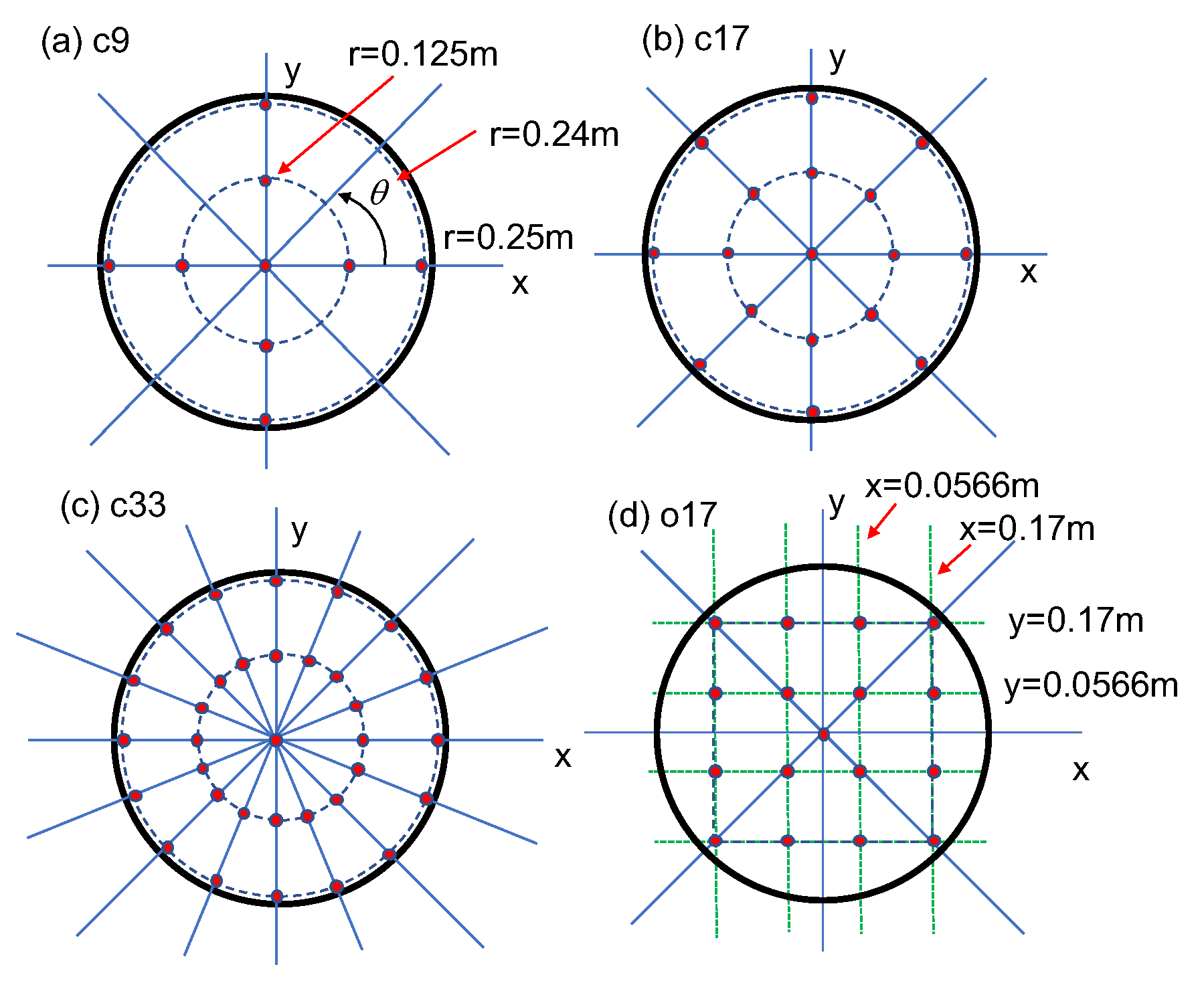
4.2. Data Assimilation Conditions

We estimated the natural convection behavior after 40.25 s by the LETKF using the base simulation results, and we applied the data assimilation (the Kalman filter update in Equation (18)) every 0.25 s. We set the number of ensemble members $m=20$, and we used every second data from 30 to 49 s of the base simulation (the data at $t=30,31,\dots ,49$ s) as the data of the initial ensemble members, that is, the ensemble members at 40 s. This is to make the initial ensemble members which satisfy the conservation laws in Equations (1)–(4). We also conducted the data assimilation in the case of $m=30$. However, there was no noteworthy difference between the analysis results for $m=20$ and $m=30$. We used the temperature T, mass fraction of helium $Y_{He}$, and density $\rho$ as the observation data. The observation data of T, $Y_{He}$, and $\rho$ were made by adding normal random numbers with standard deviations of 1.0 K, 0.0016, and $0.01$ kg/m3 to the true simulation data, respectively. The standard deviation of 0.0016 of $Y_{He}$ corresponds to the standard deviation of 0.01 of the molar fraction of helium. We assumed the observation errors were about one percent for the helium molar fraction and the density. The observations were assumed to be uncorrelated. Then, the observation covariance error matrix R was diagonal. The diagonal components of R were $1.0^2$, $0.{0016}^2$, and $0.{01}^2$ for the temperature, the mass fraction of helium, and the density, respectively. We applied four different observation locations. Observation locations in the horizontal cross-section are shown in Figure 8. The red circles in Figure 8 indicate the observation points. Figure 8a–c indicate cylindrical arrangements c9, c17, and c33. Figure 8d indicates orthogonal arrangement o17. The indices of the arrangement names show the numbers of the observation locations in the horizontal cross-section. All arrangements include the observation along the center axis. The observations are located at the radii $r=$0.125 m and 0.24 m, and in the azimuthal directions of [$\theta ={90}^{\circ }\times n(n=0,\dots ,3)$], [$\theta ={45}^{\circ }\times n(n=0,\dots ,7)$], and [$\theta =22.5^{\circ }\times n$$(n=0,\dots ,15)$] for arrangements c9, c17, c33, respectively. The observations are located at $(x,y)=(\pm 0.0566\mathrm{m},\pm 0.0566\mathrm{m}),(\pm 0.0566\mathrm{m},\pm 0.17\mathrm{m}),(\pm 0.17\mathrm{m},\pm 0.0566\mathrm{m}),$$(\pm 0.17\mathrm{m},\pm 0.17\mathrm{m})$ for arrangement o17. The observation points are located every 100 mm in the z direction. The shape of the local patch was rectangular. The dimensions of the local patch were 0.17 m in the x direction, 0.17 m in the y direction, and 0.206 m in the z direction. We set the localization length as $\sigma =0.085$ m. In this study, the noteworthy sensitivity to $\sigma$ was not observed. We used the inflation factor $\delta =0.1$.

The numerical conditions of the flow simulation and the data assimilation are summarized in

Table 3. Conditions of flow simulation and data assimilation. T: temperature, $Y_{He}$: helium mass fraction, $\rho$: density, and U: velocity.

Case	Observation Location	Boundary Condition	Analysis Objects of Data Assimilation	Objects of Observation	Interaction Froude Number
1	c17	BC 2	$T,Y_{He},U$	$T,Y_{He}$	0.73
2	c9	BC 2	$T,Y_{He},U$	$T,Y_{He}$	0.73
3	c33	BC 2	$T,Y_{He},U$	$T,Y_{He}$	0.73
4	c33-h	BC 2	$T,Y_{He},U$	$T,Y_{He}$	0.73
5	o17	BC 2	$T,Y_{He},U$	$T,Y_{He}$	0.73
6	c17	BC 1	$T,Y_{He},U$	$T,Y_{He}$	0.73
7	c33-h	BC 1	$T,Y_{He},U$	$T,Y_{He}$	0.73
8	c17	BC 2	$T,Y_{He},U$	T	0.73
9	c17	BC 2	$T,Y_{He},U$	$Y_{He}$	0.73
10	c17	BC 2	$T,Y_{He},U,\rho$	$T,Y_{He}$	0.73
11	c17	BC 2	$T,Y_{He},U,\rho$	$T,Y_{He},\rho$	0.73
12	c17	BC 2	$T,Y_{He},U$	$T,Y_{He}$	0.66
13	c17	BC 2	$T,Y_{He},U$	$T,Y_{He}$	0.89
no-DA case 1	-	BC 2	-	-	0.73
no-DA case 2	-	BC 2	-	-	0.66
no-DA case 3	-	BC 2	-	-	0.89

. Observation location c33-h indicates that the observation points are located every 20 mm in the z direction and arranged by arrangement c33 in the horizontal cross-section. In no-DA (data assimilation) case 1, the data assimilation was not applied, and the result of no-DA case 1 corresponds to the base simulation result. We investigated the sensitivities of the observation locations (c9, c17, c33, c33-h, or o17), the temperature boundary condition (BC 2 or BC 1), the analysis objects of the data assimilation ((T, $Y_{He}$, velocity U) or (T, $Y_{He}$, U, $\rho$)), and the objects of the observation ((T, $Y_{He}$), (T), ($Y_{He}$) or (T, $Y_{He}$, $\rho$)). In cases 6 and 7, we used the true simulation data at $t=30,\dots ,49$ s as the initial ensemble members to apply temperature boundary condition BC 1. Furthermore, we investigated the sensitivity of the interaction Froude number $Fr$. We applied the data assimilation to the simulations under the conditions of $Fr=0.66$ and 0.89 in cases 12 and 13, respectively. The simulations of no-DA cases 2 and 3 correspond to the base simulations under the conditions $Fr=0.66$ and 0.89, respectively.

5. Results and Discussion

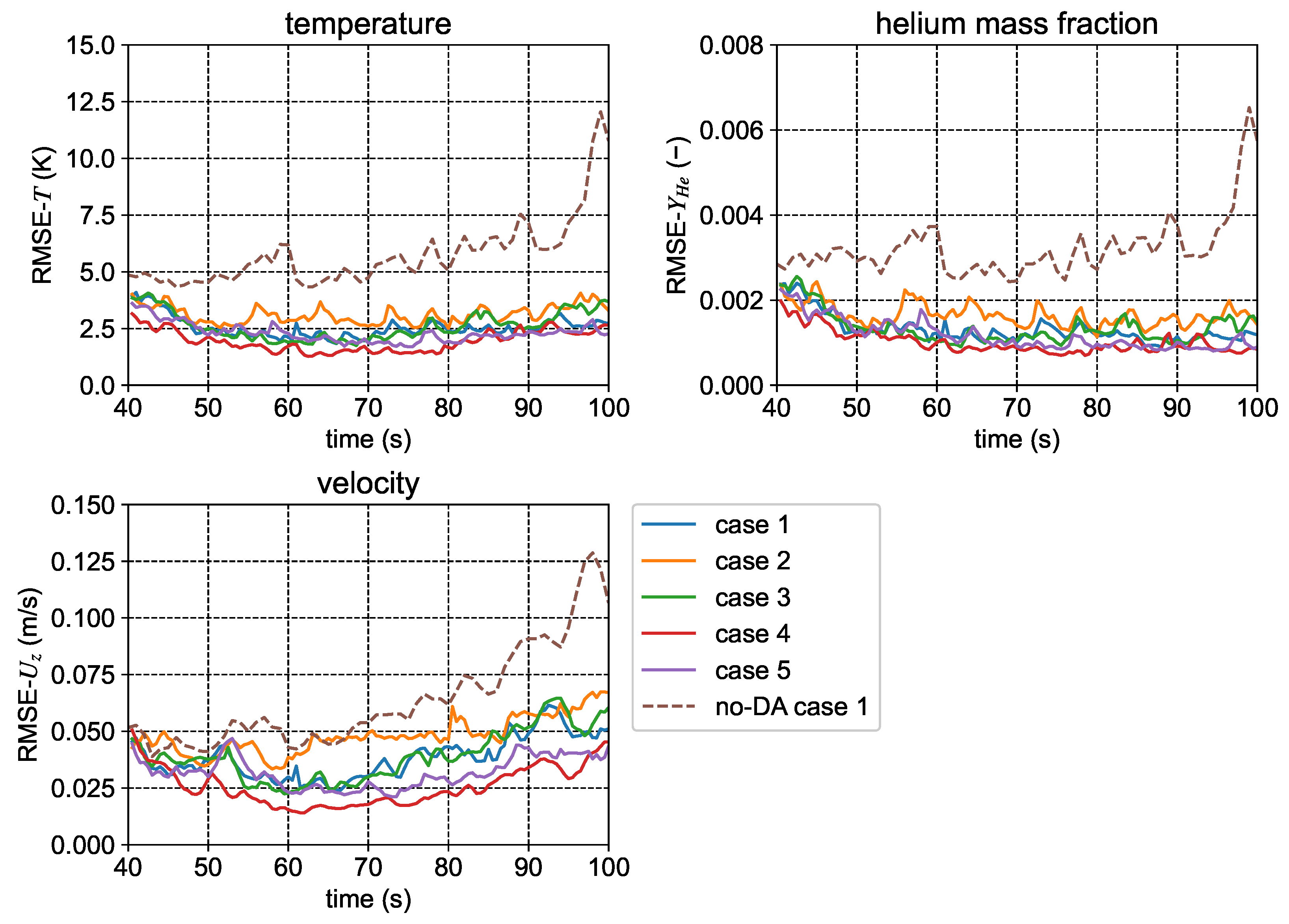
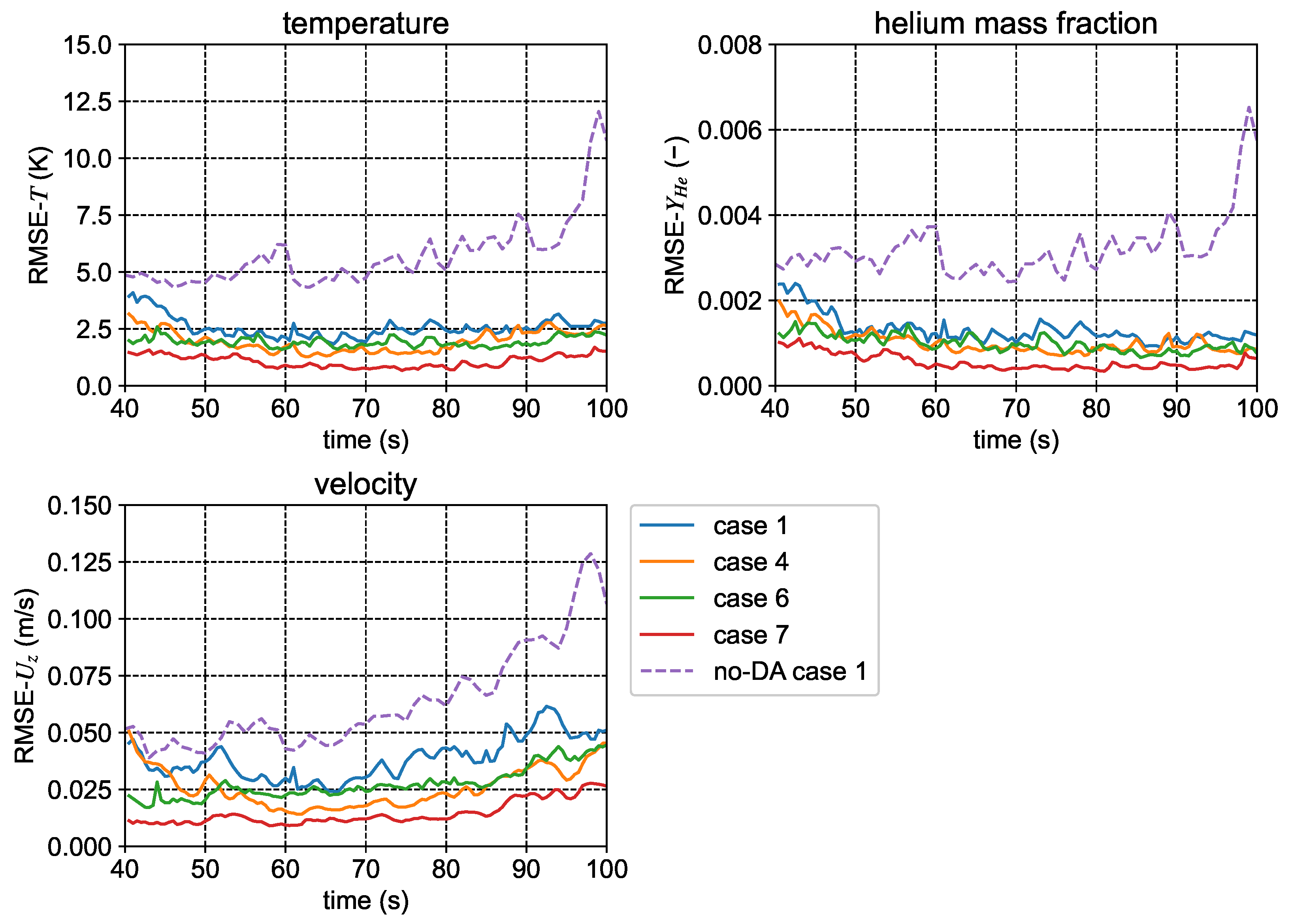
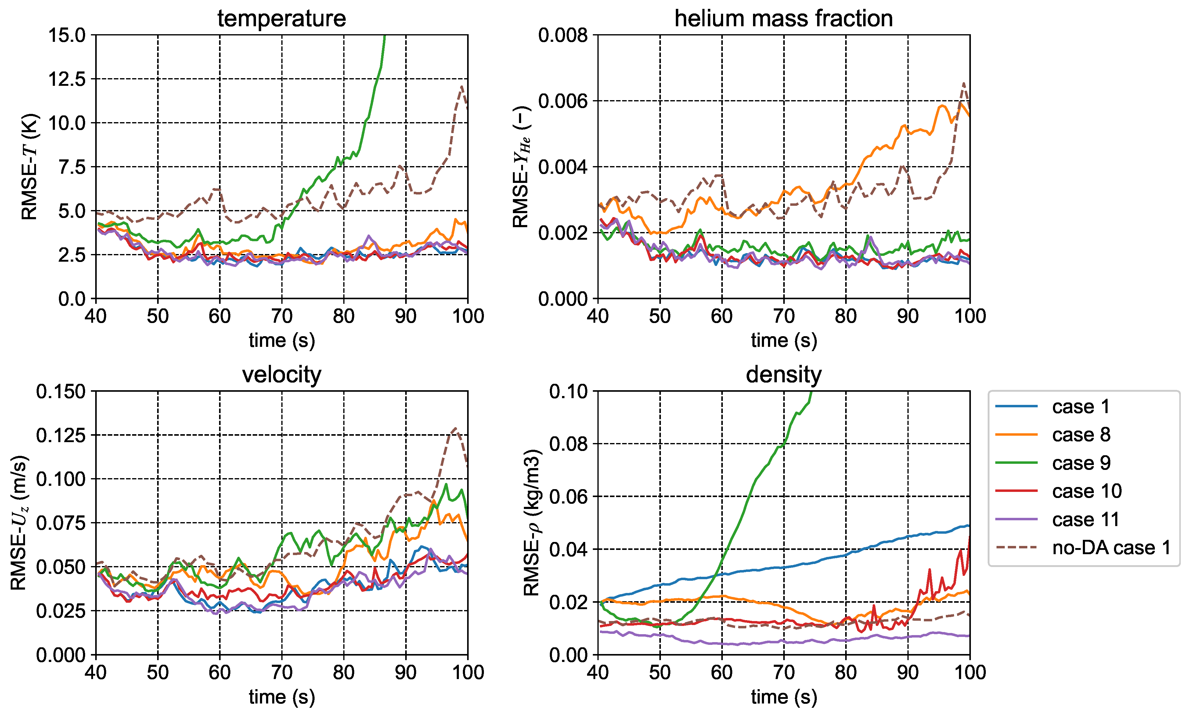
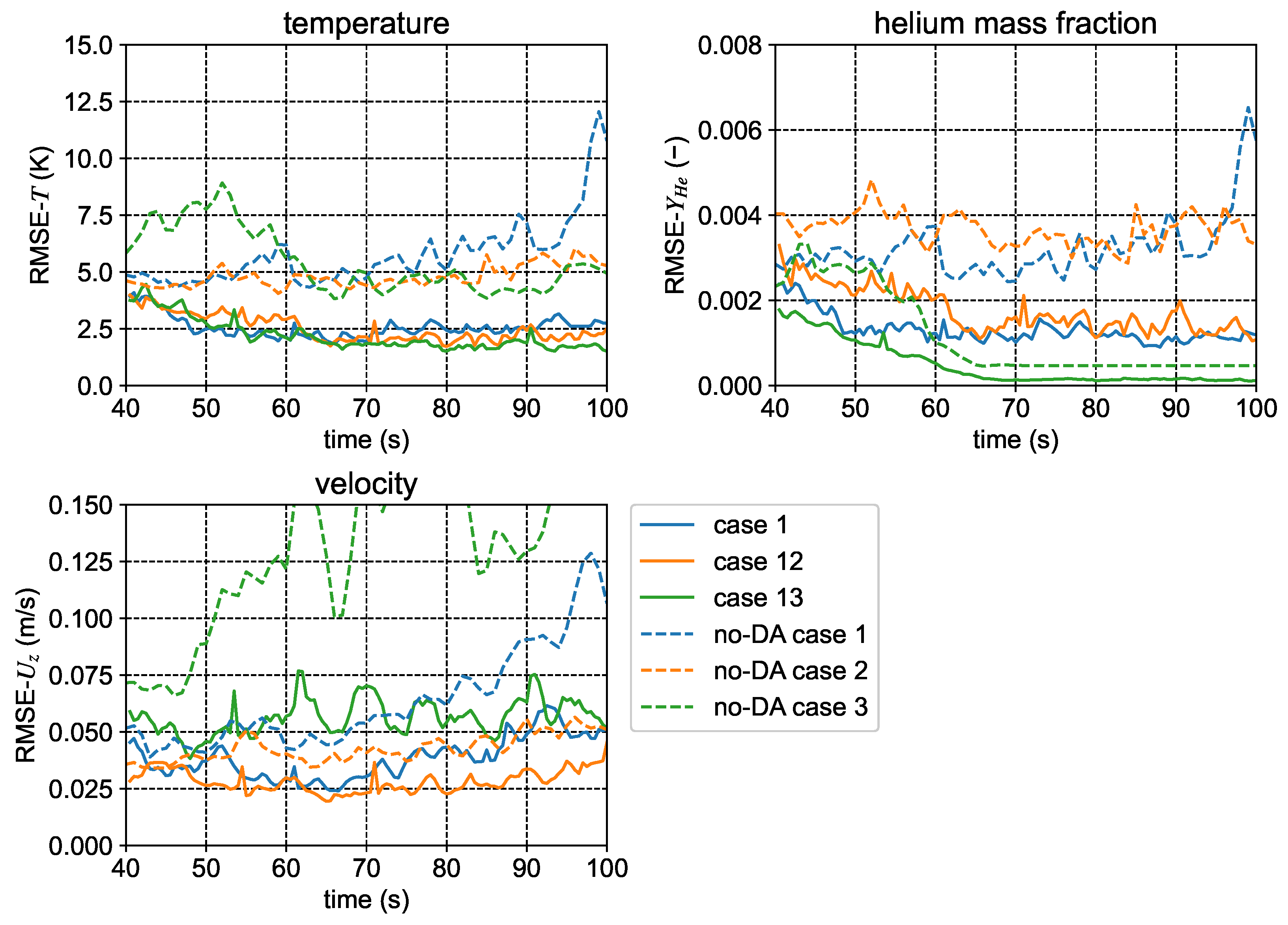
5.1. Root Mean Square Errors

The root mean square error (RMSE) between the analysis value $q^a$ and the true value $q^{true}$ is defined as below.

$$\begin{array}{c}\hfill RMS{E}_t=\sqrt{\frac{{\sum }_{l=1}^{N_{all}}{(q_{t,l}^a-q_{t,l}^{true})}^2}{N_{all}}}\end{array}$$

(20)

where $N_{all}$ is the total number of cells and $q_{t,l}$ is a physical quantity (temperature, velocity component, helium mass fraction, or density) in the l-th cell at time t. Figure 9 shows the RMSEs of the temperature, helium mass fraction, and velocity component in the z direction by using the different observation locations. The RMSEs in no-DA case 1, i.e., the RMSEs of the base simulation result under the condition $Fr=0.73$, increased rapidly after 90 s, and the RMSEs in no-DA case 1 were larger than those in the other cases where the data assimilation was applied. This result indicates the accuracy of the numerical simulation is improved by the data assimilation. The RMSEs in case 4, which had the maximum number of observation points, were the smallest during almost all time. The RMSEs in case 5 by using orthogonal arrangement o17 were slightly smaller than those in case 1 by using cylindrical arrangement c17. This is because the local patch was rectangular in shape and the observation points of arrangement o17 were evenly distributed in the local patch. A noteworthy difference in the RMSEs of the temperature and helium mass fraction was not observed in cases 1–5. Figure 10 shows the RMSEs by using the different temperature boundary conditions. In cases 1 and 4, temperature boundary condition BC 2 was applied, and in cases 6 and 7, condition BC 1 was applied. By applying the boundary condition of the true simulation, i.e., condition BC 1, the RMSEs decreased, and the accuracy of the simulation was improved. Moreover, the accuracy of not only the temperature but also the helium mass fraction was improved by applying the accurate temperature boundary conditions. This is because the convective behavior was simulated more accurately by using the accurate temperature boundary condition. Figure 11 shows the RMSEs by using the different analysis objects of the data assimilation and the different objects of the observation. The observation object in case 8 was the temperature and that in case 9 was the helium mass fraction. In case 8, the RMSE of the helium mass fraction increased to the same level as in the no-DA case 1. The RMSE of the temperature in case 9 was much larger than that in the no-DA case 1. The RMSE of the density in case 9 was significantly larger than those in the other cases. The use of the temperature data as the observation object is important for accurate analysis. The RMSE of the density in case 11 was the smallest by using the density data as the observation object. On the other hand, the RMSE of the density in case 10 was smaller than those in cases 8 and 9 during 40–75 s and almost the same value as that in case 8 after 75 s. The accuracy of the analysis can be improved by using the density as the data assimilation object, even if the density is not observed. Figure 12 shows the RMSEs under the conditions of the different interaction Froude number. The results in case 1 and no-DA case 1 show those under $Fr=0.73$. Similarly, the results in case 12 and no-DA case 2 and case 13 and no-DA case 3 show those under $Fr=0.66$ and 0.89, respectively. The RMSEs in case 12 decreased to the same level as in case 1. In case 13 and no-DA case 3, the density stratification collapsed and the gas concentration was homogenized at about 65 s, and natural convection occurred in the entire vessel. Then, the RMSE of the helium mass fraction became almost constant after about 65 s, and it was smaller than those in cases 1 and 12. The RMSEs of the temperature and the velocity in case 13 decreased to the same level as in case 1. The simulation results were improved by the data assimilation regardless of the Froude number.

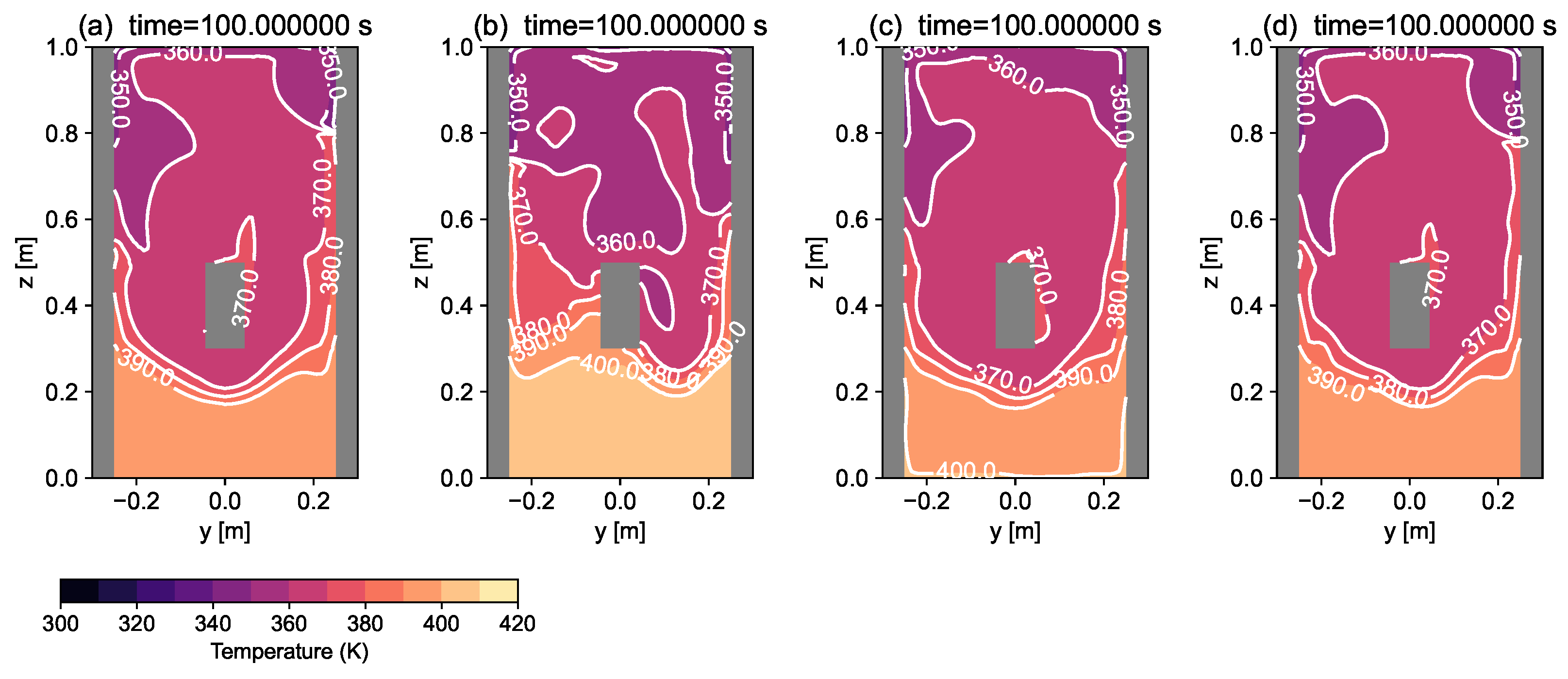
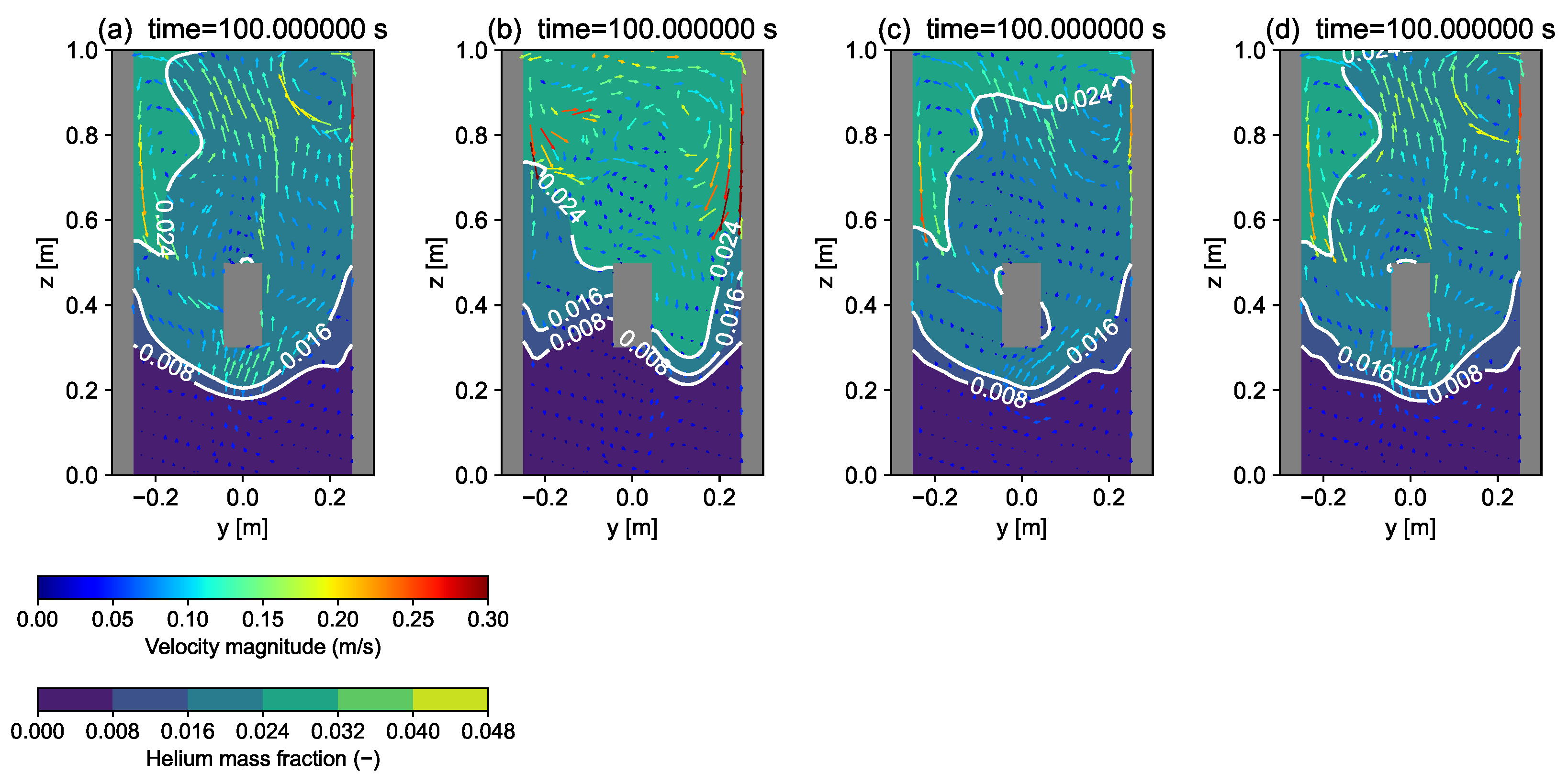
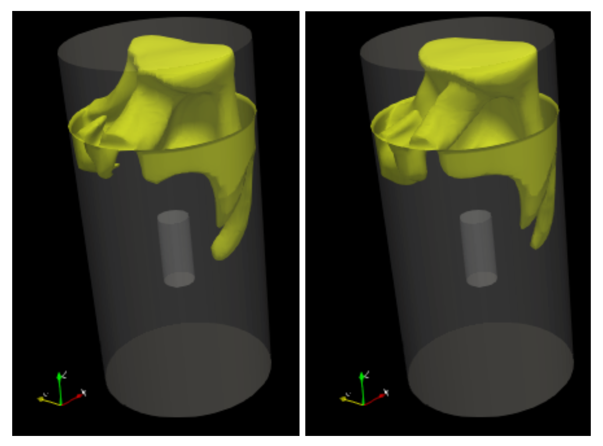
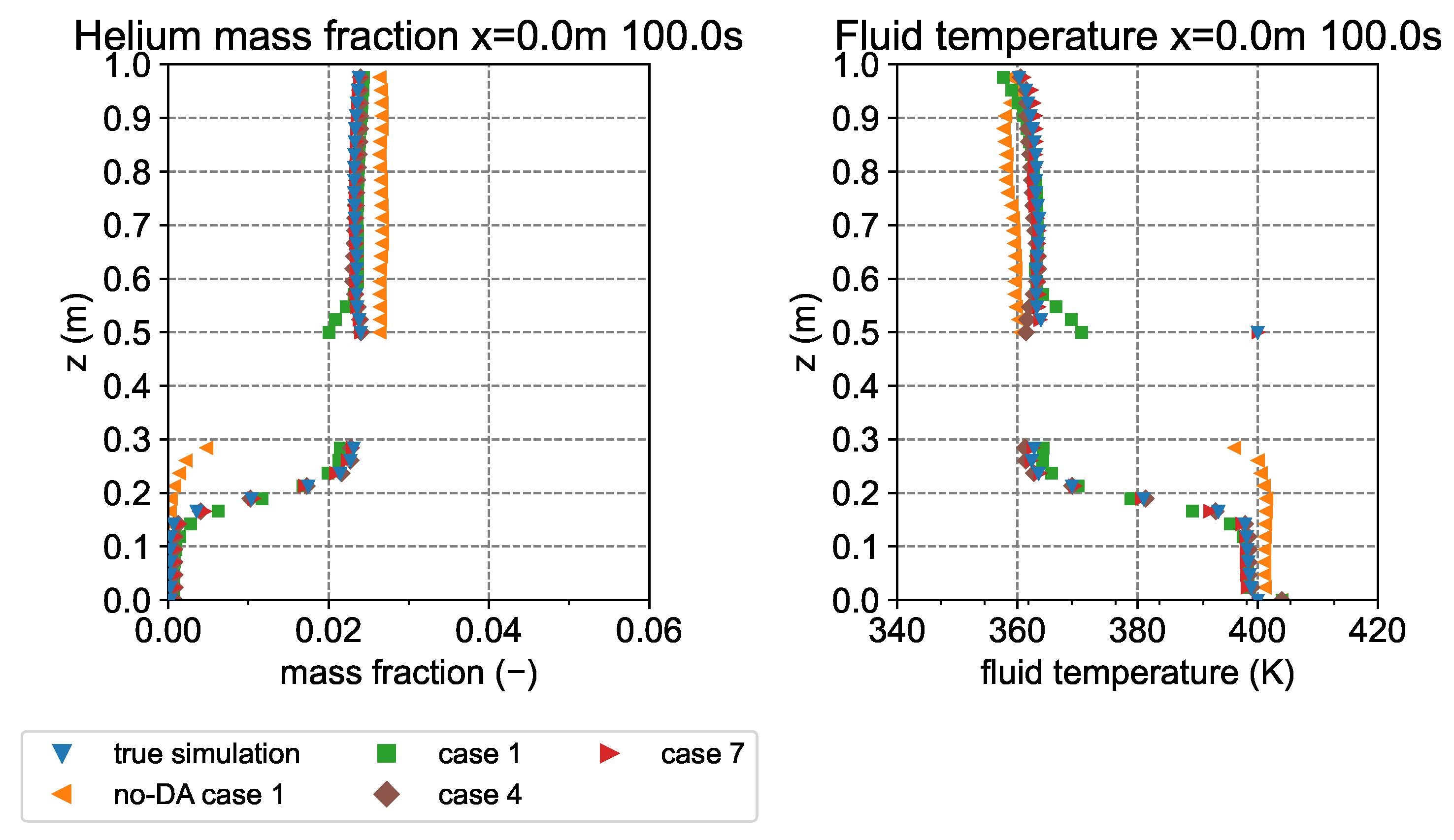
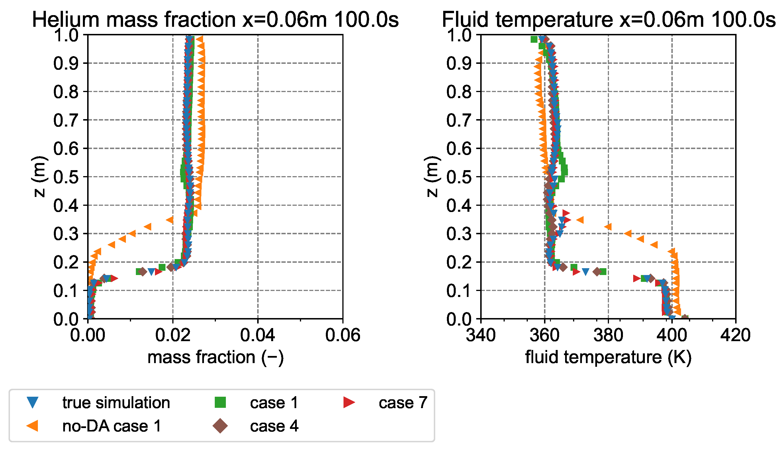
5.2. Contours and Vertical Distributions of Temperature and Helium Mass Fraction

Figure 13 and Figure 14 show the contours of the temperature and the helium mass fraction on the $yz$ plane in (a) the true simulation, (b) no-DA case 1, and (c) case 1 and (d) case 7 at 100 s. The velocity vectors are also plotted in Figure 14. The temperature contour in no-DA case 1 was significantly different from that in the true simulation. On the other hand, the temperature in case 1 almost reproduced that in the true simulation. Furthermore, the temperature in case 7 reproduced the true distribution more accurately than that in case 1. From Figure 14, the downward flow near the cold wall occurred, and complex convection flows were observed in the upper region. The helium mass fraction distribution in case 7 reproduced the true distribution more accurately than that in case 1 as well as the temperature distribution. The isosurfaces of the temperature in the true simulation and case 7 at 100 s are shown in Figure 15. The isosurface of $T=360$ K is depicted. The asymmetric and complex temperature distributions were observed. The complex flow behavior caused these complex temperature distributions. The isosurface in case 7 almost reproduced the true simulation distribution.

The vertical distributions of the helium mass fraction and the temperature along $(x,y)=(0.0\mathrm{m},0.0\mathrm{m})$ at 100 s is shown in Figure 16. Figure 16 indicates that the distributions in no-DA case 1 were significantly different from those in the true simulation. The temperature at $z=0.5$ m, i.e., the elevation at the upper surface of the injection nozzle, was not reproduced in case 1 where the base simulation boundary condition (condition BC 2) was applied. However, above $z=0.58$ m, the temperature in case 1 was almost the same as the true value. The temperature in case 1 below $z=0.3$ m, i.e., the elevation at the lower surface of the injection nozzle, was in good agreement with the true value except in the very vicinity of the nozzle surface. Because the helium mass fraction in the true simulation was higher than that in case 1 in the upper part of the nozzle, the temperature in the true simulation tended to be homogeneous. The temperature difference between case 1 and the true simulation could be caused by this tendency. On the other hand, at the bottom of the nozzle, the difference in the helium concentration between case 1 and the true simulation was small. As a result, the temperature distributions were almost the same. Figure 17 shows the distributions along $(x,y)=(0.06\mathrm{m},0.0\mathrm{m})$ at 100 s. From Figure 17, the analyses in cases 1 and 4 did not reproduce the temperature fluctuation in the z direction. On the other hand, the analysis in case 7 reproduced the temperature fluctuations. These differences in reproducibility could be attributed to the following causes. In case 1, the resolution of the observation points in the z direction was insufficient. In addition, in cases 1 and 4, the temperature boundary condition around the injection nozzle was different from that in the true simulation. However, the temperature boundary condition in case 7 was the same as that in the true simulation. Although a small difference in the vertical temperature distribution was observed, the behavior of the stratification interface could be reproduced in cases 1, 4, and 7.

6. Summary

We applied the data assimilation by the LETKF to the simulation of the natural convection with the density stratification in the small system scaled down from the large-scale containment vessel facility CIGMA considering the similarity. We discussed the performance of the data assimilation. Based on the sensitivity evaluation for the observation locations, temperature boundary conditions, and the objects of the observation, we obtained the following conclusions:

• The RMSEs decreased with more observation locations. However, the noteworthy sensitivity to the observation locations was not observed in this study.
• The RMSEs in the case using the true temperature boundary conditions were lower than those in the case using the temperature boundary conditions with the error for the true simulation. However, the RMSEs in the case using the temperature boundary conditions with the error for the true simulation decreased by the data assimilation, and the efficiency of the data assimilation was confirmed.
• To simulate the temperature and gas mass fraction accurately, the observation data of the temperature and gas mass fraction were required. Moreover, the observation data of the temperature have a noteworthy sensitivity to the RMSE of the analysis. The RMSE of the temperature increased drastically in the case that no observation data of the temperature were used.

We revealed that the accuracy of the simulations was improved by the data assimilation in this study. On the other hand, it is necessary to evaluate the performance of data assimilation for the actual containment vessel by conducting analyses with a large-scale system as a future work because the containment vessel is much larger than the present system. For the progress of the application of the data assimilation to an actual containment vessel thermal–hydraulic behavior, we have to discuss the reduction in the number of observation points as another future work. To investigate the efficiency of the data assimilation, the natural convection behavior with the density stratification was simulated, ignoring the thermal radiation effect and the steam condensation effect in this study. In the future, we will investigate the efficiency of the data assimilation considering the influence of thermal radiation and steam condensation.

References

1. Kelm, S.; Lehmkuhl, J.; Jahn, W.; Allelein, H.J. A comparative assessment of different experiments on buoyancy driven mixing processes by means of CFD. Ann. Nucl. Energy 2016, 93, 50–57. [Google Scholar] [CrossRef]
2. Ishigaki, M.; Abe, S.; Hamdani, A.; Hirose, Y. Numerical analysis of natural convection behavior in density stratification induced by external cooling of a containment vessel. Ann. Nucl. Energy 2022, 168, 108867. [Google Scholar] [CrossRef]
3. Cornick, M.; Hunt, B.; Ott, E.; Kurtuldu, H.; Schatz, M.F. State and parameter estimation of spatiotemporally chaotic systems illustrated by an application to Rayleigh–Bénard convection. Chaos 2009, 19, 013108. [Google Scholar] [CrossRef] [PubMed] [Green Version]
4. Harris, K.D.; Ridouane, E.; Hitt, D.; Danforth, C.M. Predicting flow reversals in chaotic natural convection using data assimilation. Tellus A 2012, 64, 17598. [Google Scholar] [CrossRef]
5. Reagan, A.J.; Dubief, Y.; Dodds, P.S.; Danforth, C.M. Predicting Flow Reversals in a Computational Fluid Dynamics Simulated Thermosyphon Using Data Assimilation. PLoS ONE 2016, 11, e0148134. [Google Scholar] [CrossRef] [PubMed] [Green Version]
6. Introini, C.; Lorenzi, S.; Cammi, A.; Baroli, D.; Peters, B.; Bordas, S. A Mass Conservative Kalman Filter Algorithm for Computational Thermo-Fluid Dynamics. Materials 2018, 11, 2222. [Google Scholar] [CrossRef] [PubMed] [Green Version]
7. Abe, S.; Hamdani, A.; Ishigaki, M.; Sibamoto, Y. Experimental investigation of natural convection and gas mixing behaviors driven by outer surface cooling with and without density stratification consisting of an air-helium gas mixture in a large-scale enclosed vessel. Ann. Nucl. Energy 2022, 166, 108791. [Google Scholar] [CrossRef]
8. Hunt, B.R.; Kostelich, E.J.; Szunyogh, I. Efficient data assimilation for spatiotemporal chaos: A local ensemble transform Kalman filter. Physical D 2007, 230, 112–126. [Google Scholar] [CrossRef] [Green Version]
9. Studer, E.; Brinster, J.; Tkatschenko, I.; Mignot, G.; Paladino, D.; Andreani, M. Interaction of a light gas stratified layer with an air jet coming from below: Large scale experiments and scaling issues. Nucl. Eng. Des. 2012, 253, 406–412. [Google Scholar] [CrossRef]
10. Jirka, G.H. Integral Model for Turbulent Buoyant Jets in Unbounded Stratified Flows. Part I: Single Round Jet. Environ. Fluid Mech. 2004, 4, 1–56. [Google Scholar] [CrossRef]
11. Ampofo, F.; Karayiannis, T. Experimental benchmark data for turbulent natural convection in an air filled square cavity. Int. J. Heat Mass Transf. 2003, 46, 3551–3572. [Google Scholar] [CrossRef]
12. Abe, S.; Studer, E.; Ishigaki, M.; Sibamoto, Y.; Yonomoto, T. Density stratification breakup by a vertical jet: Experimental and numerical investigation on the effect of dynamic change of turbulent Schmidt number. Nucl. Eng. Des. 2020, 368, 110785. [Google Scholar] [CrossRef]
13. Versteeg, H.K.; Malalasekera, W. An Introduction to Computational Fluid Dynamics: The Finite Volume Method, 2nd ed.; Pearson Prentice Hall: Hoboken, NJ, USA, 2007. [Google Scholar]
14. Launder, B.; Spalding, D. The numerical computation of turbulent flows. Comput. Methods Appl. Mech. Eng. 1974, 3, 269–289. [Google Scholar] [CrossRef]
15. Viollet, P.L. The modelling of turbulent recirculating flows for the purpose of reactor thermal-hydraulic analysis. Nucl. Eng. Des. 1987, 99, 365–377. [Google Scholar] [CrossRef]
16. Abe, S.; Studer, E.; Ishigaki, M.; Sibamoto, Y.; Yonomoto, T. Stratification breakup by a diffuse buoyant jet: The MISTRA HM1-1 and 1-1bis experiments and their CFD analysis. Nucl. Eng. Des. 2018, 331, 162–175. [Google Scholar] [CrossRef]
17. Venayagamoorthy, S.K.; Stretch, D.D. On the turbulent Prandtl number in homogeneous stably stratified turbulence. J. Fluid Mech. 2010, 644, 359–369. [Google Scholar] [CrossRef] [Green Version]
18. Patankar, S.V.; Spalding, D.B. A calculation procedure for heat, mass and momentum transfer in three-dimensional parabolic flows. Int. J. Heat Mass Transf. 1972, 15, 1787–1806. [Google Scholar] [CrossRef]
19. Issa, R.I. Solution of the implicitly discretised fluid flow equations by operator-splitting. J. Comput. Phys. 1986, 62, 40–65. [Google Scholar] [CrossRef]
20. OpenFOAM-2.3.x. 2015. Available online: https://github.com/OpenFOAM/OpenFOAM-2.3.x (accessed on 6 May 2022).
21. Ishigaki, M.; Abe, S.; Sibamoto, Y.; Yonomoto, T. Influence of mesh non-orthogonality on numerical simulation of buoyant jet flows. Nucl. Eng. Des. 2017, 314, 326–337. [Google Scholar] [CrossRef]
22. Jasak, H. Error Analysis and Estimation for the Finite Volume Method with Applications to Fluid Flows. Ph.D. Thesis, The University of London, London, UK, 1996. [Google Scholar]
Figure 1. Schematic views of the vessel. (a) overhead view and (b) cross-section view.
Fluids 07 00237 g001
Figure 2. Flow chart of the twin model experiment.
Fluids 07 00237 g002
Figure 3. Simulation flow charts of the true and base simulations.
Fluids 07 00237 g003
Figure 4. Overhead and cross-section views of mesh 2. Left: overhead view and right: cross-section view.
Fluids 07 00237 g004
Figure 5. The helium mass fraction and the temperature distributions of the true simulation by using the different mesh resolutions at 15 s.
Fluids 07 00237 g005
Figure 6. Time histories of the vertical distributions of the helium mass fraction, temperature, and density by the true simulation.
Fluids 07 00237 g006
Figure 7. Distributions of the helium mass fraction for the base and true simulations at 15 s.
Fluids 07 00237 g007
Figure 8. Observation locations in the horizontal cross-section. The red circles indicate the observation points.
Fluids 07 00237 g008
Figure 9. RMSEs by using the different observation locations.
Fluids 07 00237 g009
Figure 10. RMSEs by using the different temperature boundary conditions.
Fluids 07 00237 g010
Figure 11. RMSEs by using the different analysis objects of the data assimilation and the different objects of the observation.
Fluids 07 00237 g011
Figure 12. RMSEs under the conditions of different interaction Froude numbers.
Fluids 07 00237 g012
Figure 13. Temperature contours at 100 s. (a) the true simulation, (b) no-DA case 1, (c) case 1, and (d) case 7.
Fluids 07 00237 g013
Figure 14. Helium mass fraction contours and velocity vectors at 100 s. (a) the true simulation, (b) no-DA case 1, (c) case 1, and (d) case 7.
Fluids 07 00237 g014
Figure 15. Isosurfaces of temperature at 100 s. Left: the true simulation and right: case 7.
Fluids 07 00237 g015
Figure 16. Vertical distributions of the helium mass fraction and the temperature along ( x , y ) = ( 0.0 m , 0.0 m ) .
Fluids 07 00237 g016
Figure 17. Vertical distributions of the helium mass fraction and the temperature along ( x , y ) = ( 0.06 m , 0.0 m ) .
Fluids 07 00237 g017