Numerical Simulations of the Flow Dynamics in a Tube with Inclined Fins Using Open-Source Software

Abstract

Finned tubes increase the convective heat transfer in heat exchangers, reducing the total energy consumption of integrated industrial processes. Due to its stability and robustness, Computational Fluid Dynamics (CFD) commercial software is generally utilized for analyzing complex systems; however, its licensing is expensive. Nowadays, open-source software is a viable substitute for proprietary software. This work presents a CFD analysis of the hydrodynamics of a finned tube using the OpenFOAM and SALOME Meca platforms. The results are compared with experimental data and CFD using the commercial software Fluent, both previously reported in the open literature. This work studies the fluid flow pattern around a tube with six 45-degree-angled fins, and the working fluid, air, is considered as an incompressible fluid. Special attention is paid to calculating the pressure coefficient distribution for the internal and external surfaces of the inclined fins. Open-source platforms allow researchers to visualize how the airflow interacts with the cylinder and the fin surfaces to form a fluid structure, formerly known as a horseshoe vortex system. The findings of the analysis of flow dynamics in the channel between inclined fins and in the wake help explain the results obtained in experimental tests and are relevant for the configuration of a bank of tubes with inclined fins.

1. Introduction

Extended surfaces have many applications such as in heat recovery boilers, air-cooled heat exchangers, and others [1]. Annular and spiral finned tube banks are the most used extended surfaces, and the methodologies for calculating heat transfer and pressure drop on these surfaces are well known [2,3]. These methodologies have their origin in the experimental studies of the flow dynamics and the local heat transfer, both in the channel formed by two fins and in the cylinder. The importance of the secondary flow that develops at the junction of the fin with the tube and its interaction with the shear layers that separate from the fin surface forming complex three-dimensional structures were identified. For example, the horseshoe vortex system develops during the interaction between the cylinder and the fluid flow [4,5]. Consequently, the structure of the wake and its behavior are more complex than those observed in banks of smooth tubes [6].

Modifications to annular or spiral fins have been proposed to enhance convective heat transfer [7,8,9], primarily to perturb the flow, destroy the boundary layer, or generate secondary flow [10]. To obtain a comprehensive explanation of the complex mechanism that enhances heat transfer in this kind of extended surfaces, experimental investigations are not enough.

The computational fluid dynamics (CFDs) technique has proven to be a useful tool for analyzing convective heat transfer in finned tubes [11], as well as in plate fin-tube heat exchangers [12], in the study of compact heat exchangers [13] and the analysis of flow dynamics on extended surfaces with complex geometry, such as crimped spiral fins, wavy fins, plain fins with a delta winglet pair, and serrated fins [14,15].

However, despite the increase in heat transfer obtained by a bank of tubes with inclined or conical fins when compared to a bank of tubes with a plain circular fin with an equivalent area [15], there is a lack of numerical studies of flow dynamics and heat transfer in tubes with inclined fins. As far as the authors know, there is only one work on this topic in the last 20 years [16].

In line with the above, the motivation of this article is to perform numerical modeling on the flow dynamics in a tube with 45-degree inclined fins, using open-source software, and compare the results to both experimental and proprietary software results.

The article is organized into three sections. Section 2 presents the experimental study’s findings. Section 3 presents the results of the numerical investigation conducted using the proprietary program fluent. Section 4 of the paper discusses the computational calculations of the flow dynamics in the tube with inclined fins and in the wake development. Finally, in Section 5, the findings of both numerical simulations are compared with the physical experimental data of the pressure coefficient distribution.

2. Experimental Investigation

In an earlier work [9], the specifics of the experimental configuration and the model of the tube with inclined fins were described. The tube with inclined fins had an external diameter of D = 42 mm, and five fins, with a h = 16 mm distance between them, were attached to it. The fin length was H = 20 mm and the thickness was δ = 2 mm. The experimental set up consisted of an induction wind tunnel with a test section of 950 mm length and 120 × 106 mm cross-section; it had an inlet profile to smooth the flow. The tube with inclined fins was installed at the center of the test section and was exposed to an air crossflow.

An inclined manometer consisting of 19 tubes, each with a diameter of 1.2 mm, was used to measure static pressure. Pressure taps, with a diameter of 0.3 mm, were distributed on the internal and external surfaces of an inclined fin: 8 pressure taps on each face and 3 pressure taps on the tube. Because the space around the root and the edge of the fin was limited, pressure measurements begin at 20% and end at 90% of total fin length which correspond to 0.004 and 0.018 m, respectively.

To analyze the relative pressures throughout the flow field using the experimental results, the pressure coefficient was calculated using the following equation.

$$c_p=\frac{p-p_0}{q},$$

(1)

where $p$ is the static pressure, $p_0$ is the operation pressure, and $q$ is the dynamic pressure.

As is well known, the distribution of the pressure coefficient, $c_p$, on a surface can be used to reconstruct the flow dynamics by the interaction of flow and surface. The pressure coefficient, $c_p$, distribution on the external and internal face of the inclined fin is shown in Figure 1a,b, respectively, with a Reynold’s number of Re = 56,000.

As observed in Figure 1, the pressure coefficient distribution on both surfaces is quite different.

The $c_p$ distribution presented by the internal surface, Figure 1a, follows a non-linear trend. In the region at an internal face with a rotational angle of 0 to 140 degrees, the maxima and minima were recognized. On the other hand, $c_p$ was constant across the length of the fin when the rotation angle was between 150 and 170 degrees. Finally, at 180 degrees, a maximum developed near the back of the fin, indicating the countercurrent flow effect in this area.

The $c_p$ distribution in the external surface of the inclined fin shown in Figure 1b followed a quasi-linear trend with a distinctive slope up to 90 degrees of rotation, as expected. In the range of 100 to 130 degrees, the $c_p$ did not change the length of the fin. Furthermore, a positive value of the pressure coefficient was preserved up to 50 degrees of rotation, before reverting to negative values. This shows how far the primary flow’s impact extends before being replaced by the secondary flow that forms and develops near the back of the inclined fin.

The experimental results presented in [9] were not to fully describe the flow dynamics in the channel between two inclined fins as well as in the tube’s wake. Therefore, it was necessary to carry out a numerical study.

3. Numerical Simulations with Proprietary Software

A numerical study of the flow dynamics in a tube with inclined fins was first attempted by Garcia-Figueroa [16]. The numerical simulations using the FLUENT (v. 6.1) proprietary platform were performed on a 32-bit PC with 1GB of RAM, Pentium 4 processor at 2.6 Ghz, and Windows XP Professional as the operating system.

The numerical model was modeled using a rectangular duct with 0.06 m × 2.02 m × 0.031 m. The rectangular section allowed one half to be simulated in one channel of fins. Symmetry planes were imposed to the system to obtain the results and the three-dimensional flow behavior was simulated with limitations.

The geometry was modeled and meshed using Gambit 2.04. In the discretization of the domain, the smallest element had a volume of 6.74 × 10⁻¹⁴ m³, and in all circumstances, the distance from the first element to the fin wall was 5.00 × 10⁻⁵ m.

Table 1. Different types of discretization on the numerical model using proprietary software.

Mesh	Discretization Cells	Turbulence Model	Simulation Run Time
1	271,328	Reynold’s Stress Model	8 h
2	523,780	Reynold’s Stress Model	16 h
3	631,900	Reynold’s Stress Model	19 h

shows the number of elements used in three different meshes with proprietary software. This was performed to ensure the independence of the results with the different types of mesh. After comparisons were made, it was found that the greatest variation was 25% between cases 1 and 2 and was 2% between cases 2 and 3. Therefore, the mesh with 631,900 cells was selected to present the results for proprietary software.

Seven distinct turbulence models were used to perform numerical simulations: the Spalart-Allmaras model, the κ-ε standard model, the κ-ε RNG model, the κ-ε realizable model, the κ-ω standard model, the κ-ω SST model, and the Reynold’s stress model. After comparisons of the numerical results of all the turbulence models were made with the experimental results, the Reynold’s stress model was found to obtain the best results. In RSM numerical simulations, the model considers the turbulence anisotropy, allowing greater accuracy to be obtained in vortexes with higher dimensions than the minimum size of the elements that form the mentioned secondary flows.

Figure 2 show an isometric view using path lines colored by the particle ID to show the flow characteristics. The finned cylinder walls were colored in black to contrast with the colors of the lines and improve the visibility of the information. The figure used lines to show the results; however, they did not describe the interaction between the fluid and the structure at the edge of the fins and the flow behavior between the fin channels. The lines pass through the finned array at the center of the geometry and then move around the geometry. The flow then forms different magnitude eddies at the back of the finned cylinder at every channel.

The obtained results with the proprietary software allowed the pressure coefficient at the external and internal faces of the finned cylinder, as well as the three-dimensional flow behavior with the stationary formulation, to be visualized. Back in 2006, the hardware limitations required the operational conditions to be modified in order to perform a numerical simulation.

To gage a complete study of the flow dynamics, the three-dimensional geometry of the experimental setup must be implemented and non-stationary formulation in the numerical simulations needs to be used. In the present work, these necessary conditions were considered and implemented using the open-source software as follows.

4. CFD Analysis Using Open-Source Software

The first component of this sub-section, which is divided into three parts, gives the boundary conditions that were determined from the experimental setup, as described in a prior study [9]. The properties of the grids helped to achieve the independence of results using various meshes, as demonstrated in Section 4.2. The constitutive equations are described in Section 4.3.

The simulations using the open-source platform (v. 9) were run on a 64-bit workstation with 64 GB of RAM, one AMD Ryzen Threadripper 3960 × 24 core processor, one NVIDIA GeForce RTX 3070 GPU, and Ubuntu 20.04 LTS as the operating system. A parallelized computation was used to achieve numerical convergence, with all processes and normalized residuals having values smaller than 1 × 10⁻⁶ at each time step.

4.1. Boundary Conditions

The numerical case is located inside a rectangular computational domain and is based on the experimental work reported by Carvajal-Mariscal et. Al. [9], in which a rectangular duct has a centered and finned cylinder, and a cross flow passes around it, as described in Section 2. The experimental conditions were used as inlet boundary conditions of the numerical model. The temperature of the air was 293.15 K at 1 atmosphere of pressure, and the inlet constant velocity was 21.333 m·s⁻¹, corresponding to the experiment’s Reynold’s number of 56,000.

Figure 3 depicts the geometrical properties of the finned cylinder; the numerical model has the same dimensions as in the physical experiment. The numerical model was solved in the open-source OpenFOAM CFD toolbox [17]. The inlet was defined as the “turbulentInlet” boundary condition, with a magnitude value of 21.333 m·s⁻¹. The outlet was selected as “inletOutlet”. The internal and external fin surfaces, the walls of the cylinder, and the walls of the control volume were imposed as isothermal and non-slip boundary conditions.

To make the numerical findings easier to visualize, each of the cylinder’s seven channels were defined separately. For the total pressure, the inlet condition was defined as the “zeroGradient”, and the outlet condition was defined as the “fixedValue” with a uniform value of 0. All the walls of the system were defined as the “zeroGradient” condition.

In the “k” file, the following conditions were used. For the inlet, the type was “fixedValue”, with a uniform value of 1.706. For the outlet, the type was “inletOutlet”, with a uniform value of 0. The walls were defined as “fixedValue”, with a uniform value of 0. The turbulent kinetic energy was calculated using the following equation.

$$\kappa =\frac{3}{2}{\left(I\left|{\mathit{u}}_{inlet}\right|\right)}^2,$$

(2)

where $I$ denotes turbulence intensity and 0.05 was the chosen value. In this situation, the inlet velocity of 21.333 m s⁻¹ serves as the reference value for Equation (2).

For epsilon, the boundary conditions were as follows. For the inlet, the type was “fixedValue”, with a uniform value of 46.729. For the outlet, the type was “inletOutlet”, with a uniform value of 46.729. For the walls, the type was “epsilonWallFunction”, with a uniform value of 46.729.

Equation (3) is used to estimate the turbulence specific dissipation rate.

$$\epsilon =\frac{C_{\mu }^{0.75}{\kappa }^{1.5}}{L},$$

(3)

$C_{\mu }$ is constant with a 0.09 value and $L$ is a reference length scale with a 0.00459 value.

The inlet’s boundary condition was specified as “fixedValue”, with a uniform value of 1. The outlet condition type was inletOutlet, with a uniform value of 0. The walls were described as “zeroGradient”.

In the “nut” file, the boundary condition has one inlet and one outlet that were both defined as “zeroGradient”. The walls of the system were also declared as “zeroGradient”.

The nuTilda file has one inlet condition declared as “fixedValue”, with a uniform value of 0. The outlet boundary condition type was “inletOutlet”, with a uniform value of 0, and the walls of the system was “fixedValue”, with a uniform value of 0. When it was possible, the boundary conditions for the turbulence model were taken from the experimental data.

4.2. Discretization

The geometry and discreti-zation processes were completed using the open-source software Salome 9.8.0 as shown in Figure 4 [18]. The NETGEN 1D-2D-3D algorithm was used to mesh the geometry. A 3D hypothesis was selected. Three different finite volume meshes were used, with OpenFOAM to obtain the convergence analysis.

Table 2. Different types of discretization on the numerical model using open-source software.

Mesh	Tetrahedrons Volumes	Nodes	Turbulence Model	Simulation Run Time
1	1,461,658	250,918	Spalart-Allmaras DDES	0.5 h
2	2,609,918	450,270	Spalart-Allmaras DDES	1 h
3	4,079,020	658,959	Spalart-Allmaras DDES	1.5 h

shows the most relevant information of the discretization process to reach the independency of the results with different meshes.

Numerous criteria must be met using the control volume mesh. The locations of the separation points and contact points have a significant impact on the distribution of pressures on the geometry’s surfaces. Therefore, it is important that the control volume mesh resolves these pertinent geometry-related details and complies with the specifications of the physical models used in the simulation.

For flows with a high Reynold’s number, resolving the near-wall region down to the sub-viscous layer is not a viable choice because of the unreasonably high number of cells needed in that region. Since they are sensitive to the effects of pressure gradients, the unbalanced function’s wall treatment will be applied to circumvent this restriction. They consider the impacts of local variations in the sub-viscous layer thickness when calculating the turbulent kinetic energy in cells next to the walls and draw comparisons to the wall functions. They are also sensitive to unbalanced wall functions. Without significantly increasing calculation time or dynamic memory, they offer more accurate forecasts of turbulent boundary layer behavior, including the wake.

Using the appropriate values of y⁺ close to the model’s walls is the first step in determining the size of an average element [19]. To obtain an initial distribution of the volume mesh, this value is allocated to all the geometry’s edges afterwards. The level of resolution needed for the simulation must first be established, as well as the available computational power.

Given that the distance between the fins in this example is 1.6 × 10⁻² m, the length of the first cell, when assuming an air flow rate of 21.333 m·s⁻¹, may be too long; Since exterior flows are recognized to be those in which the control volume’s walls have little to no impact on the flow around the body being investigated, they do not apply to the current scenario but can still be used as a starting point. The y⁺ value is determined using Equation (4).

$$y^{+}=\frac{\sqrt{\rho \tau }}{\mu }{y}_p,$$

(4)

where $\mu$ is the dynamic viscosity, $\rho$ is the density, $\tau$ is the shear stress in the wall, and $y_p$ is the distance from the wall to the cell node. Additionally, since y⁺ Equation (4) depends on the wall stress and the effective viscosity, both of which are computed and changed throughout the calculation process in each iteration, it cannot be applied.

The Salome’s platform adaptability functionality is used in a meshing technique [18]. As a starting point, a rather coarse mesh is created, and a first solution is computed. Several modifications that consider the static pressure gradients and mesh refinement are required to complete this solution. Once the ultimate answer is found, the cycle is repeated while the solution continues. This technique cannot be applied in this work because the phenomena are complicated and the pressure and velocity gradients are very large, and because making many adjustments greatly increase the number of nodes.

For the meshing technique used in this work, in the first stage, a viscous layer was defined around the finned cylinder shape walls in the software’s hypothesis selection. Ten layers were used, and the total thickness of the layers was 1 mm with a stretch factor of 1. A surface offset and smooth extrusion method was selected to continue with the meshing process around the finned cylinder and therefore to the rectangular volume. After that, the finite volume mesh was converted with the “ideasUnvToFoam” command, and the result was used in the OpenFOAM solver.

4.3. Constitutive Equations

The flow was governed by the Navier–Stokes equation that expresses the conservation of mass and momentum expressed in Equations (5) and (6). The flow was assumed to be incompressible, and the fluid was treated as ideal gas with properties evaluated at $T_0$ = 293.15 K.

$$\nabla ·\mathit{u}=0,$$

(5)

$$\rho \left(\frac{\partial \mathit{u}}{\partial t}\right)+\mathit{u}·\nabla \mathit{u}=-\nabla p+\nabla ·\left[\mu \left(\nabla \mathit{u}+{\left(\nabla \mathit{u}\right)}^T\right)\right]+\rho \mathrm{g},$$

(6)

The semi-implicit method for pressure-linked equations is an algorithm used for steady-state solutions. The κ-ε and κ-ω turbulence models were solved using the simpleFOAM solver [20,21,22]. This method eliminates the time derivative term from the equations and solves the pressure and momentum equations on the following iterations.

The pressure-implicit split operator algorithm, which is also a finite volume discretization method used for incompressible, unsteady, and three-dimensional flow, was utilized as a second approach. The PisoFOAM solver was used with the Spalart–Allmaras DDES model [23].

The Spalart–Allmaras DDES model is a one-equation model based on a modified turbulence viscosity, $\tilde{v}$, and on the Spalart–Allmaras DES model. This turbulence model is suitable for 3D cases and transient numerical simulations, but not for cases with smaller dimensions [17].

The transport equation for the Spalart–Allmaras model is given by Equation (7).

$$\frac{D}{Dt}\left(\rho \tilde{v}\right)=\nabla ·\left(\rho D_{\tilde{v}}\tilde{v}\right)+\frac{C_{b2}}{{\sigma }_{v_t}}\rho {\left|\nabla \tilde{v}\right|}^2+C_{b1}\rho \tilde{S}\tilde{v}\left(1-f_{t2}\right)-\left(C_{w1}{f}_w-\frac{C_{b1}}{{\kappa }^2}{f}_{t2}\right)\rho \frac{{\tilde{v}}^2}{{\tilde{d}}^2}+S_{\tilde{v}},$$

(7)

The model equations are the same as in the DDES variation, but the length scale $\tilde{d}$ approximation is different, as shown in Equation (8).

$$\tilde{d}=max\left({\mathrm{L}}_{RAS}-f_d,max\left({\mathrm{L}}_{RAS}-{\mathrm{L}}_{LES},0\right)\right),$$

(8)

The large eddy simulation (LES) length is

$${\mathrm{L}}_{LES}={\mathsf{\Psi }\mathrm{C}}_{DES}\Delta ,$$

(9)

The delay function is given by

$$f_d=1-tanh\left[{\left(C_{d1}{r}_d\right)}^{C_{d2}}\right],$$

(10)

when $f_d=0$, RAS is recovered, and when $f_d=1$, then the DDES mode is recovered. The $r_d$ parameter is given by:

$$r_d=min\left(\frac{v_{eff}}{\left|\nabla \mathit{u}\right|{\kappa }^2{y}^2},10\right),$$

(11)

The low Reynold’s number correction function Ψ is given by Equation (12)

$${\mathsf{\Psi }}^2=min\left[{10}^2,\frac{1-\frac{1-C_{b1}}{C_{w1}{\kappa }^2{f}_w^{*}}\left[f_{t2}+\left(1-f_{t2}\right)f_{v2}\right]}{f_{v1}max\left({10}^{-10},1-f_{t2}\right)}\right],$$

(12)

The open-source platform was used to solve the numerical case using the κ-ε and κ-ω turbulence models, and steady conditions were applied to bring the solution into convergence. When the results from both turbulence models were compared to those from the proprietary platform, no qualitative difference was found.

The case was solved using three different inlet velocities that were 10 percent up and down from the experimental inlet flow condition. In this study, a single inlet velocity, the same as the experimental results that were previously published, was reported in this work [9]. Convergence was reached in each case when these operating conditions were resolved using the Spalart–Allmaras DDES turbulence model.

Thus, the Spalart–Allmaras DDES turbulence model was selected because it yields more accurate results at non-steady conditions. The greater number of elements used in the discretization step is one of the key factors. The DDES model only solves one constitutive equation and greatly speeds up computation. For instance, the total calculation time in Table 2 is shorter than in Table 1 for the smallest case using the proprietary platform.

5. Results and Discussion

In this section, the authors discuss their analysis of the flow dynamics around the finned cylinder geometry in Section 5.1. A comparison between the experimental technique data and two numerical simulations techniques is presented in Section 5.2.

5.1. Flow Dynamics Analysis

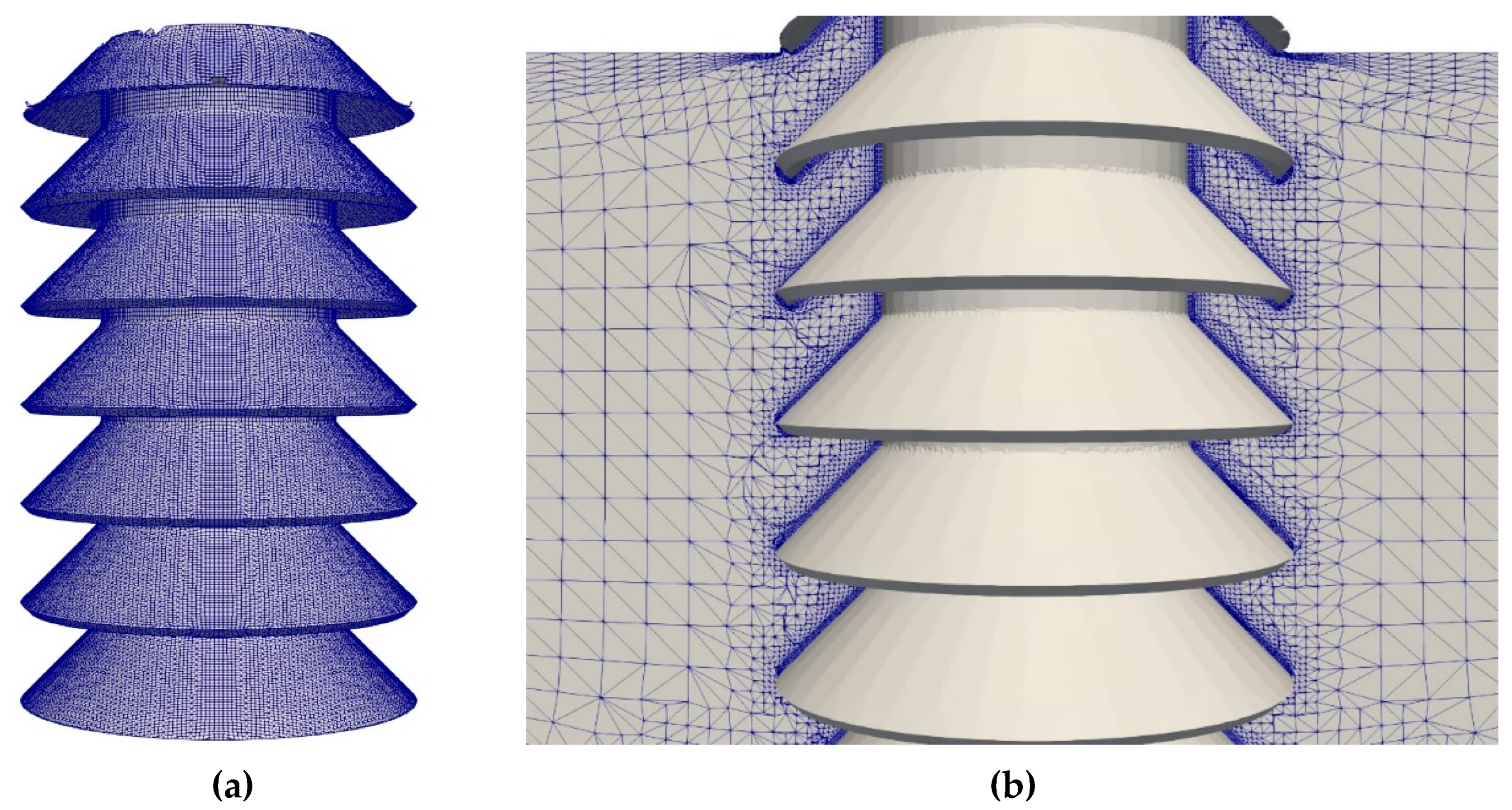
The geometry in this section was designed using an open-source program without any simplifications or symmetry planes. Using the SALOME platform (v. 9.8.0), the discretization’s element density was significantly higher than the grid utilized with proprietary software. Substantial benefits were observed using the open-source platform; for example, it is possible to study the three-dimensional flow behavior and the wake development that occurs between the channels of fins using non-steady numerical simulations. The results of the numerical simulations that were calculated using OpenFOAM are presented. (The section on Supplementary Materials has a download link for an animation of the three-dimensional flow behavior at three different angles. This animation uses an open-source platform to make it simpler to visualize and understand the results of non-steady state numerical simulations.)

The calculation process completed 20 s. The figures depict the flow behavior at different process times, as well as the development of the flow along the duct. A quasi-stationary flow behavior was established after the initialization of the simulation. Approximately 10 s of process were necessary to observe stable flow conditions in the simulation analysis.

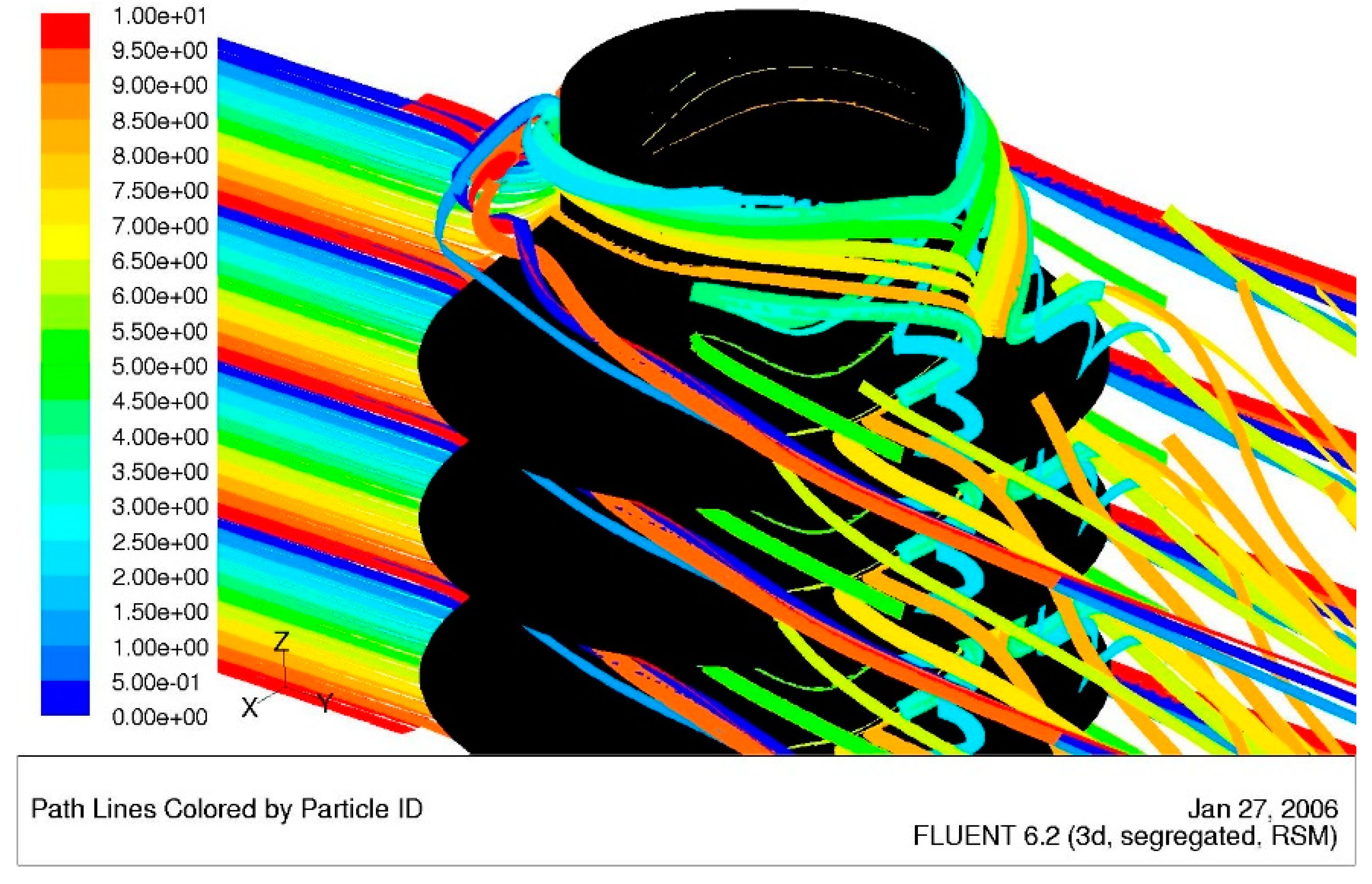
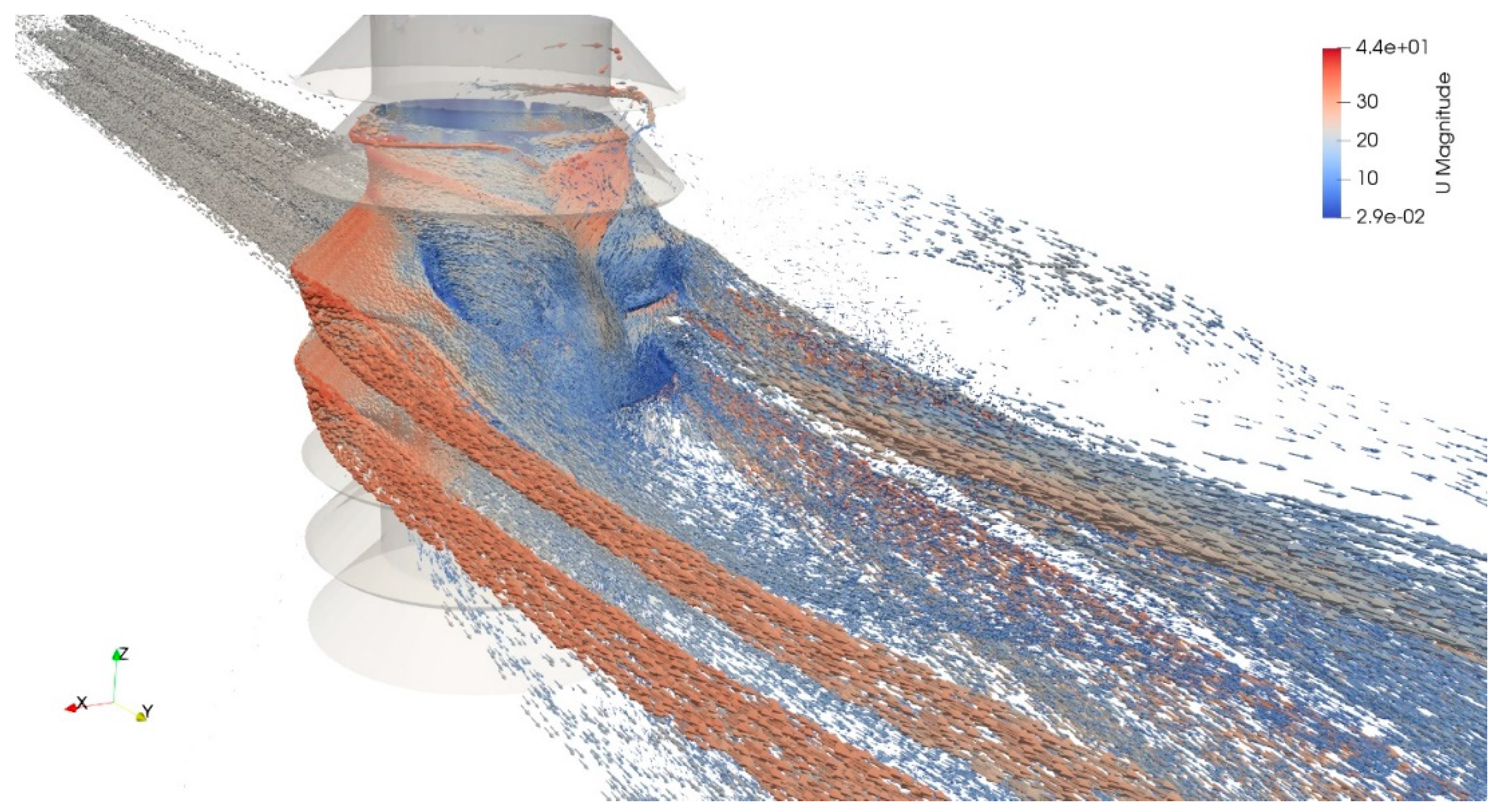
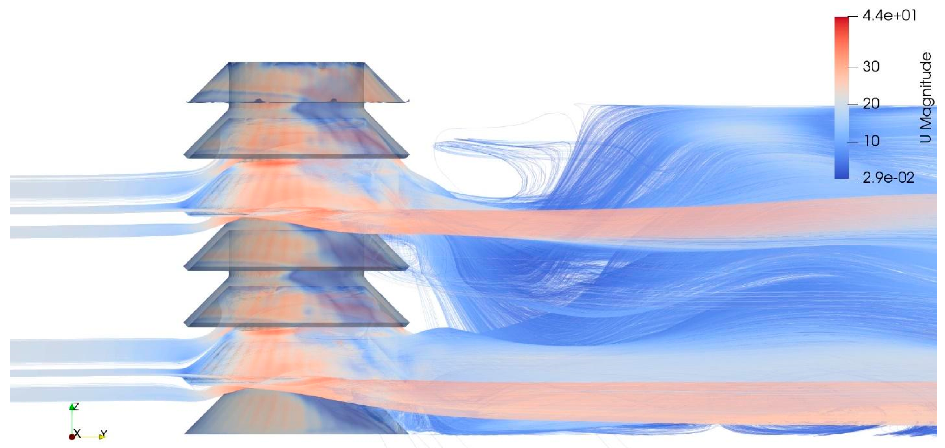
Figure 5 uses an isometric back perspective of the numerical simulation results to depict the fourth and fifth channel of fins attached to a cylinder. The flow hits the angled fins and flows horizontally close to the fin’s edge, as shown by 3D vectors colored by flow velocity magnitude; meanwhile, below the fin, at the internal wall, the flow interacts and generates a high turbulent flow stream. At φ = 0°, the flow passes through the fin, and at approximately φ = 110°, one horseshoe vortex system (HVS) forms at each fin’s channel. The flow interacts with the finned cylinder walls and high velocity streams just after the cylinder achieves a low-velocity area.

Between the lateral walls of the control volume and the fin edges, 0.5 equivalent diameters were defined on each lateral side. There were no significant changes in the flow behavior due to the wall’s influence in this study.

The flow velocity magnitude colors the fin surfaces. The flow separation sites can be identified by the color variations on the cylinder and fin. Because of the turbulence, the flow stream direction changes, and oscillations are detected throughout the simulations.

A second smaller HVS was discovered and grown around the cylinder between the fifth and sixth channel fin. The fourth channel flow interacts with the fifth channel flow, but the flow structure in each channel appears to be autonomous and is not totally absorbed by the generated turbulence behind the cylinder.

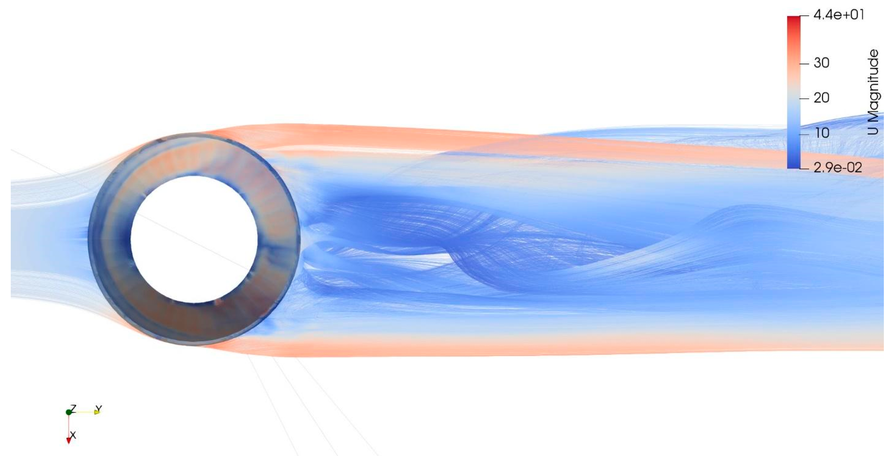
In Figure 6, which depicts the top view of the control volume, the flow passes along the fourth channel of the cylinder fins. Although a large amount of data was collected, the third and fourth fin channel streamlines are shown in this figure to make visualization easier.

Because the angle of the fins and the vertical cylinder walls vary the flow direction, the flow enters the control volume at the inlet wall, interacts with the finned cylinder, and generates turbulence along the duct. The velocity magnitude of the flow colors the cylinder fin surfaces, resulting in a non-uniformity distribution along the surface. From φ = 0°, the flow decelerates along the fin surface, splitting into two lateral streams, and then accelerates and separates from the fin’s surface between φ = 95° and φ = −95°.

The finned cylinder is followed by a turbulent wake. A symmetric flow pattern was identified in this perspective, although the produced turbulence surrounding the fins constantly changes the wake.

The separation point is where the flow separates from the cylinder or the surface of the fins. In this situation, there are two pairs of separation points. The first pair occurs between φ = 40 and φ = 50 degrees, as well as φ = −40° and φ = −50°. Between φ = 100° and φ = 115° and φ = −100° and φ = −115°, the second pair appears.

The flow passes around the finned cylinder, forming the wake with two lateral flow streams at φ = 45° and φ = −45°, with an approximately larger flow velocity magnitude, as shown in Figure 6. The horseshoe vortex system is the flow behavior that swirls and continues forward in the wake. At varying channels of fins, the low velocity center flow streams interact.

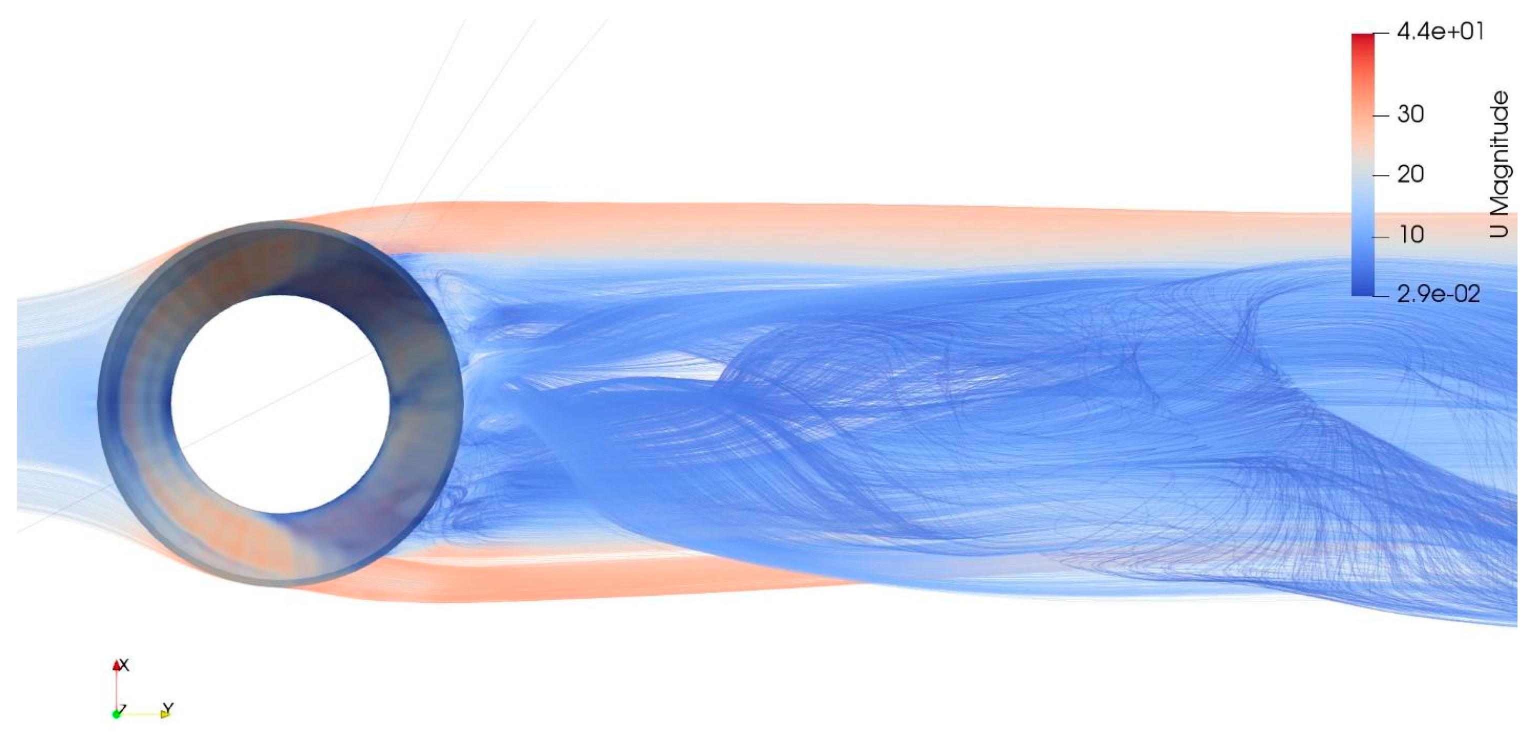
Figure 7 depicts the bottom viewpoint of the simulation at the same time. Because of the finned cylinder’s vertical location, the flow stream passes between the third and fourth channel of fins and splits into two lateral streams. The flow swirls and produces the HVS, and high-velocity flows move from the region near the cylinder to the immediate region at the base, causing a localized area of increased turbulence.

The HVS is continuously developed because of the formation of unsteady vortices at the front side of the cylinder. Streamwise streaks and turbulent structures are also developed at the end of the control volume. The streams between channel interacts behind the cylinder and develops highly turbulent structures. At two equivalent distance diameters in the wake, a high turbulence zone can be observed because of the flow interaction with the cylinder.

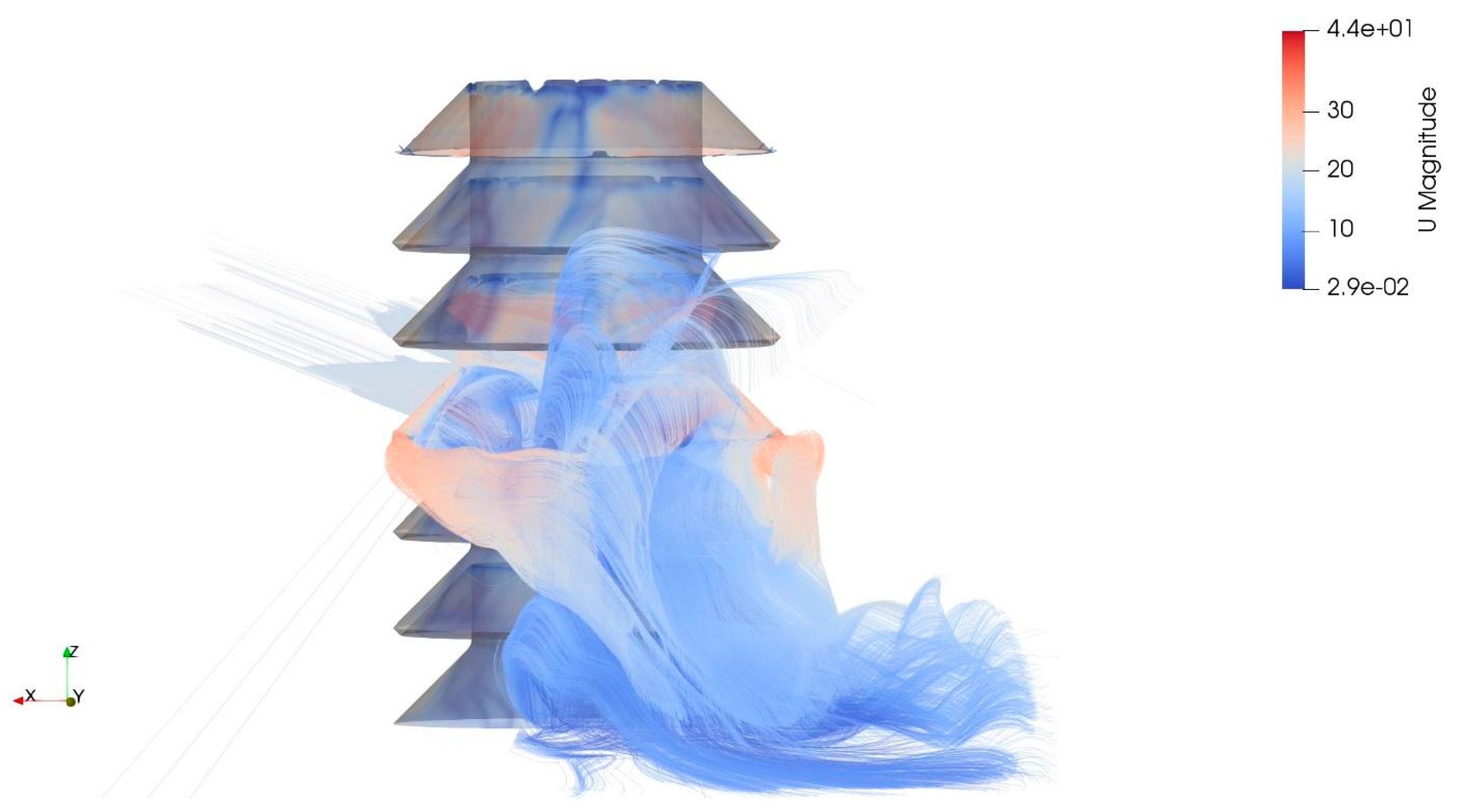
Figure 8 shows the simulations result of the wake; in this viewpoint, it is possible to observe that the flow in the wake moves downwards, and the interaction of this turbulent flow will interact with the lower channel fin flow. The HVS leads the flow downwards. Behind the cylinder, an upward flow stream in the wake is also observed that interacts with the next HVS channel. The downward flow hits the bottom wall of the volume and then moves forwards close to the wall.

The information obtained from Figure 6, Figure 7 and Figure 8 shows that there is no interaction of the flow with the control volume’s lateral walls. On each side, the cylinder and the volume walls are separated by 0.5 of the cylinder’s equivalent diameter. The velocity magnitude inlet condition prevents the flow from moving to the volume’s walls. Additionally, Figure 8 illustrates that the wake does not extend beyond the diameter of the finned cylinder.

Figure 9 depicts two distinct wake patterns of two fin channels. The flow passes through the fins on the second and fifth channels and around the cylinder. The wake from the second channel flows downward and upward; meanwhile, the wake from the fifth channel tends to move upward. The interaction of the two wakes increases the turbulence, and this structure occupies the remaining volume after one equivalent diameter distance. This figure shows that the horseshoe vortex separates from the fin surface edge and also demonstrates how its structure is maintained along the wake. Although the velocity distribution on each fin differs, the hydrodynamics in each channel are comparable.

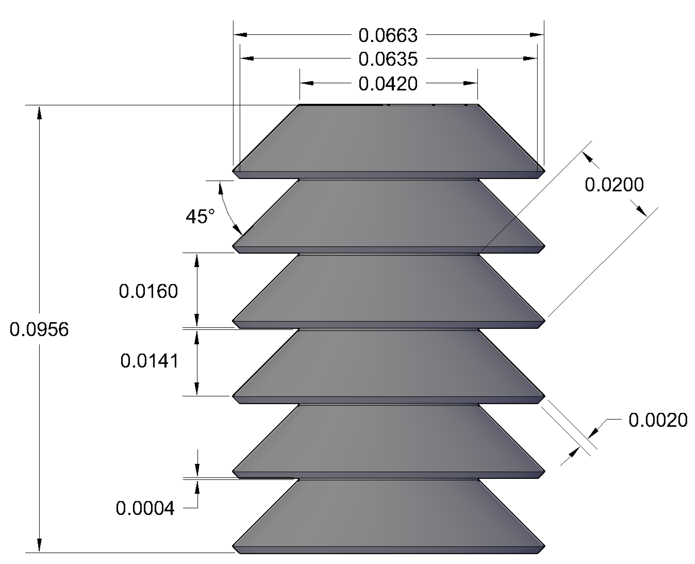
It is worth noting that the finned cylinder ends in the experimental setup were built to eliminate junctions between the fin and wind tunnel surfaces. In the numerical model, the surfaces of the fin and cylinder were combined to prevent the turbulence at the edges of the first and the last fin channels.

5.2. Comparison between Experimental and Numerical Techniques

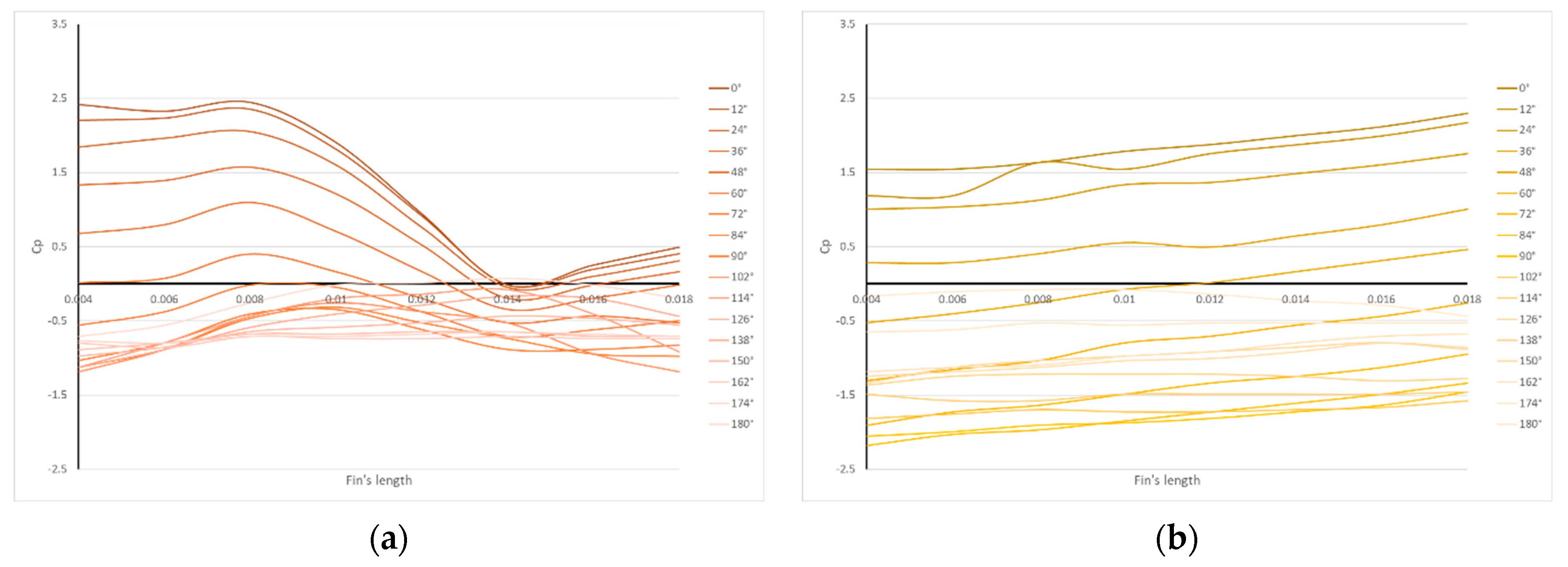
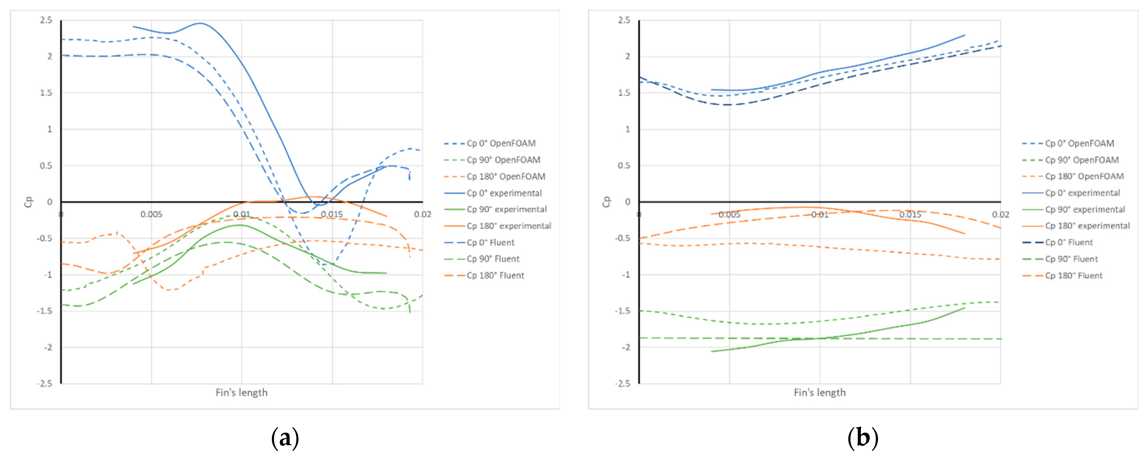
The results of the numerical simulation were compared with the results of the prior experiment. For the internal and external surfaces of the fin, three distinct rotation angles were used, 0, 90, and 180 degrees, which corresponded to the frontal, lateral, and back regions, respectively, of the inclined fin. The following equation was used to calculate the pressure coefficient in numeric computations.

$$c_p=\frac{p_{gauge}}{0.5·u_{inlet}^2},$$

(13)

Figure 10 shows the length of the fin on the x axis and the $c_p$ value at φ = 0°, φ = 90°, and φ = 180° on the y axis. It is feasible to see that the length of the curves in numeric results is longer than that of the experimental results. It was possible to insert a 3D line in numeric results and retrieve results all along the fin. On the contrary, it was difficult to install the pressure taps and their tubes inside the limited space of the inclined fin, particularly at the root and edge zones of the fins, as mentioned in Section 2.

Figure 10a shows the $c_p$ distribution on the internal surface of the inclined fin. The numeric and experimental results have similar trends in the frontal region of the inclined fin. The numeric results underestimate the experimental data, from 0.0075 to 0.014 m of the fin’s length, with a difference of 35%, bringing the OpenFOAM results closer. On the other hand, after 0.014 m, the FLUENT results have a negligible difference with respect to the experimental results, while the OpenFOAM results underestimate them with a maximum difference of 48%.

The $c_p$ values for lateral and back regions range from 0 to −1.5, but there are differences in the fluctuations between the two regions. The curves depict a normal distribution behavior at the lateral region. The $c_p$ defines a concave downwards behavior at the back region. The numerical results have a similar pattern to the experimental findings in both regions; however, the differences are distinct for each software. In the lateral region, the FLUENT results show a minimum difference of 5% and a maximum of 34%, while the OpenFOAM results show 12% and 40%, respectively. In the back region, the FLUENT results show a minimum difference of 5% and a maximum of 25%, while OpenFOAM results show 25% and 40%, respectively. The flow behavior condition and the non-steady condition utilized in the numerical simulations could be used to explain the disparities between the experimental and numerical methodologies.

$c_p$ in the lateral region has the lowest value out of the three studied regions. The $c_p$ values are closed to 0 at the back region; moreover, the $c_p$ value at this region yields the greatest difference between the two approaches, numerical and experimental, because turbulence is larger in this zone. It is reasonable to suppose that the numerical simulations’ deviations are greater because of these flow circumstances.

Figure 10b shows the pressure coefficient values at the external surface of the fourth channel fin calculated from experimental data and numerical calculations for the frontal region, colored in blue; the lateral region, colored in green; and the back region, colored in orange. On the external surface, at lateral and back regions, there were variations between the experiment and the computations. Because of the interaction with the cylinder walls, there are significant flow changes at this zone due to turbulence.

The trend of the experiment curve is comparable to the numerical techniques at the frontal region, as shown in 10b, and the differences between the results are less than 5%. The curve shape is comparable in both ways at the lateral region. The OpenFOAM results show a minimum difference of 3% and a maximum of 20%, while the FLUENT results show 13% and 24%, respectively. In the back region, the curves resembled each other in shape. The OpenFOAM results show a minimum difference of 18% and a maximum of 34%, while the FLUENT results show 12% and 18%, respectively. The magnitude difference between the two procedures is larger than in the previous two regions.

The numerical simulations using proprietary software were performed using the Reynold’s stress model (RSM) turbulence model. Based on Garcia-Figueroa’s work, the RSM obtained the best results of seven different turbulence models using the same proprietary software [16]. The RSM considers the turbulence anisotropy to model the vortexes and the hydrodynamic flow behavior. This feature offers several advantages in comparison to other turbulence models.

Proprietary software has multiple benefits. For example, it is possible to use different types of turbulence models in one study case. However, it also has some limitations. One of these limitations is the total number of elements used in one case. For academic licensing, the grid limitation could be greater than the student license. The discretization limitation in proprietary software should be considered when deciding between open-source and proprietary software. Because of the turbulent nature of the hydrodynamics in the case presented in this work, the grid resolution allows the regions over the fin surface to be located where the wake is developed. The flow behavior in the wake is important when an array of tubes is configured.

Although proprietary software provides several advantages, it also several limitations, including the total amount of elements that can be used in a single case. The grid restriction could be changed because of the licensing type. When choosing between proprietary and open-source software in CFD numerical simulations, the discretization restriction in proprietary software may be a crucial factor. The grid resolution in this study’s case, using the open-source platform, allows researchers to identify the areas over the fin surface where the wake develops due to the turbulent character of the hydrodynamics. This result could not be obtained in the proprietary platform because of the lower number of elements. Is also important to mention that the turbulence model applied in every case could be essential to approach the numerical results in the experimental data.

In this study, different turbulence models were used in the open-source and the proprietary platform. In OpenFOAM, the turbulence model used was Spalart–Allmaras DDES, while in Fluent, the RSM was the turbulence model. Based on the findings in Figure 10, it is feasible to compare the two numerical approaches and indicate that the open-source platform was able to replicate the time variations seen during the experiment. These changes have a significant impact on the results and possibly make it challenging to simultaneously compare the fluctuations in the pressure coefficient distribution over time from three distinct rotation angles. An averaged result might replicate the overall flow behavior across the cylinder, just as the proprietary program did.

Important information regarding the flow behavior was shared by the results from this work using both proprietary and open-source software. As a final remark, it was shown that the open-source platform allows a large element count to be reached, as well as the grid’s topological properties. Moreover, the chosen turbulence model could obtain crucial flow behavior data, which was not possible with commercial software.

6. Conclusions and Recommendations

In this study, experimental and numerical techniques were used to collect the data required to comprehend and accurately describe the three-dimensional flow behavior of a turbulent airstream passing through a seven-channel finned cylinder using proprietary and open-source software.

Two different turbulence models were applied in numerical simulations. As was previously reported in other work, the Reynold’s stress model used in the proprietary software reproduced the averaged flow behavior and the generalized flow conditions observed in the experiments. However, it was not possible to determine, for example, the position where the flow separates from the fin surface. This information was used for the design of the heat transfer equipment. The Spalart–Allmaras DDES turbulence model used in the present work with the open-source platform reproduced the time-related variations of the turbulent flow observed in physical experiments.

Utilizing open-source software enables the solution of various license constraints, such as the number of elements of discretization process. In fact, in this work, it was possible to replicate the results obtained with commercial software while utilizing platforms such as OpenFOAM.

The flow visualization used in this work with open-source software could help to identify the previously reported horseshoe vortex system formed around the finned cylinder, and could corroborate the symmetry of flow behavior over the fin surfaces as well as the flow characteristics at the wake.

A comparison between the experimental data and the numerical techniques shows that both techniques have differences with the physical information, mainly to do with the generated turbulence. The minimum difference between experimental data and OpenFOAM was 3%, and the maximum difference was 48%. Despite these differences, the open-source platform reproduced the complex flow dynamics of the studied case.

References

1. Pongsoi, P.; Pikulkajorn, S.; Wongwises, S. Heat Transfer and Flow Characteristics of Spiral Fin-and-Tube Heat Exchangers: A Review. Int. J. Heat Mass Transf. 2014, 79, 417–431. [Google Scholar] [CrossRef]
2. Pis’mennyi, E.; Polupan, G.; Carvajal-Mariscal, I.; Sanchez-Silva, F.; Pioro, I. Handbook for Transversely Finned Tube Heat Exchanger Design; Academic Press: Cambridge, MA, USA, 2016; ISBN 9780128043974. [Google Scholar]
3. Pis’Mennyi, E.N.; Terekh, A.M.; Polupan, G.P.; Carvajal-Mariscal, I.; Sanchez-Silva, F. Universal Relations for Calculation of the Drag of Transversely Finned Tube Bundles. Int. J. Heat Mass Transf. 2014, 73, 293–302. [Google Scholar] [CrossRef]
4. Baker, C.J. The Turbulent Horseshoe Vortex. J. Wind. Eng. Ind. Aerodyn. 1980, 6, 9–23. [Google Scholar] [CrossRef]
5. Baker, C.J. The Oscillation of Horseshoe Vortex Systems. J. Fluids Eng. 1991, 113, 489–495. [Google Scholar] [CrossRef]
6. Pis’mennyi, E.N. An Asymptotic Approach to Generalizing the Experimental Data on Convective Heat Transfer of Tube Bundles in Crossflow. Int. J. Heat Mass Transf. 2011, 54, 4235–4246. [Google Scholar] [CrossRef]
7. Pis’Mennyi, E.N. Heat Transfer Enhancement at Tubular Transversely Finned Heating Surfaces. Int. J. Heat Mass Transf. 2014, 70, 1050–1063. [Google Scholar] [CrossRef]
8. Sayed Ahmed, S.A.E.; Mesalhy, O.M.; Abdelatief, M.A. Flow and Heat Transfer Enhancement in Tube Heat Exchangers. Heat Mass Transf. 2015, 51, 1607–1630. [Google Scholar] [CrossRef]
9. Carvajal-Mariscal, I.; Sanchez-Silva, F.; Quinto-Diez, P. Flow Dynamics between the Inclined Fins of a Finned Tube. Int. J. Heat Fluid Flow 2001, 22, 519–524. [Google Scholar] [CrossRef]
10. Schlichting, H. Boundary Layer Theory, 7th ed.; McGraw-Hill: New York, NY, USA, 1979. [Google Scholar]
11. Stark, J.R.; Bergman, T.L. Prediction of Convection from a Finned Cylinder in Cross Flow Using Direct Simulation, Turbulence Modeling, and Correlation-Based. Methods Numer. Heat Transf. Part A Appl. 2017, 71, 591–608. [Google Scholar] [CrossRef]
12. Şahin, H.M.; Dal, A.R.; Baysal, E. 3-D Numerical Study on the Correlation between Variable Inclined Fin Angles and Thermal Behavior in Plate Fin-Tube Heat Exchanger. Appl. Therm. Eng. 2007, 27, 1806–1816. [Google Scholar] [CrossRef]
13. Adam, A.Y.; Oumer, A.N.; Najafi, G.; Ishak, M.; Firdaus, M.; Aklilu, T.B. State of the Art on Flow and Heat Transfer Performance of Compact Fin-and-Tube Heat Exchangers. J. Therm. Anal. Calorim. 2020, 139, 2739–2768. [Google Scholar] [CrossRef]
14. Kumar, A.; Joshi, J.B.; Nayak, A.K. A Comparison of Thermal-Hydraulic Performance of Various Fin Patterns Using 3D CFD Simulations. Int. J. Heat Mass Transf. 2017, 109, 336–356. [Google Scholar] [CrossRef]
15. Salinas-Vázquez, M.; Ramírez-Cruz, J.; Vicente, W.; Martínez-Espinosa, E.; Aviña-Jiménezez, H.M.; Lagarza-Cortés, C. Large Eddy Simulation of Fully-Developed Flow in a Helical Segmented-Fin Tube Bundle. Appl. Math. Model. 2021, 98, 595–610. [Google Scholar] [CrossRef]
16. Garcia-Figueroa, J.R. Simulacion Numerica de La Dinamica de Flujo Alrededor de Un Tubo Con Aletas Inclinadas a Distintos Angulos. Master’s Thesis, Instituto Politecnico Nacional, Mexico City, Mexico, 2006. [Google Scholar]
17. Greenshields, C. OpenFOAM v9 User Guide; The OpenFOAM Foundation: London, UK, 2021. [Google Scholar]
18. Commissariat à l’Energie Atomique et aux Energies Alternatives; EDF R&D. Open Cascade Salome6 the Open-Source Integration Platform for Numerical Simulation 2022. Open Cascade: Paris, France. Available online: https://www.salome-platform.org/ (accessed on 5 January 2021).
19. von Karman, T. Turbulence and Skin Friction. J. Aeronaut. Sci. 1934, 1, 1–20. [Google Scholar]
20. Launder, B.E.; Spalding, D.B. The Numerical Computation of Turbulent Flows. Comput. Methods Appl. Mech. Eng. 1974, 3, 269–289. [Google Scholar] [CrossRef]
21. Spalart, P.R.; Allmaras, S.R. One-Equation Turbulence Model for Aerodynamic Flows. Rech. Aerosp. 1994, 1, 5–21. [Google Scholar]
22. Vieser, W.; Esch, T.; Menter, F. Elements of Industrial Heat Transfer Prediction. In Proceedings of the 16th Brazilian Congress of Mechanical Engineering (COBEM), Uberlandia, Brazil, 26–30 November 2001; pp. 26–30. [Google Scholar]
23. Langley Research Center Turbulence Modeling Resource. Hampton, Virginia, United States. Available online: https://turbmod-els.larc.nasa.gov/ (accessed on 5 January 2021).
Figure 1. Experimental results of the pressure coefficient distribution: (a) internal surface and (b) external surface of the inclined fin.
Fluids 07 00282 g001
Figure 2. Numerical results using proprietary software. Isometric view of path lines colored by particle ID.
Fluids 07 00282 g002
Figure 3. Schematic representation of the finned cylinder with dimensional characteristics in meters.
Fluids 07 00282 g003
Figure 4. Discretization of the numerical model (a) finned cylinder volume mesh; (b) viscous layer mesh at central longitudinal plane.
Fluids 07 00282 g004
Figure 5. Isometric rear view with vectors colored by its velocity magnitude around the fourth and fifth fin of the cylinder.
Fluids 07 00282 g005
Figure 6. Top view of streamlines colored by magnitude of velocity. The air only travels through the third and fourth fin of the tube and develops along the control volume to improve visibility.
Fluids 07 00282 g006
Figure 7. The third and fourth fin channels can be seen at the bottom of the control volume. The Spalart-Allmaras DDES turbulence model colors streams based on their velocity magnitude.
Fluids 07 00282 g007
Figure 8. Rear view showing the fourth fin height streamlines colored by their velocity magnitude that passes through the cylinder and develops along the control volume.
Fluids 07 00282 g008
Figure 9. Lateral view showing streamlines colored by their velocity magnitude. To facilitate the visualization, at inlet, the air only passes through the second and fifth fin of the tube.
Fluids 07 00282 g009
Figure 10. Pressure coefficient distribution obtained with experimental and numerical techniques at three different rotation angles: 0, 90, and 180 degrees. (a) Internal surface; (b) external surface of the inclined fin.
Fluids 07 00282 g010