Validation of the LOGOS Software Package Methods for the Numerical Simulation of Cavitational Flows

Abstract

Verification problems and numeric simulation of cavitation processes with the help of LOGOS computational fluid dynamics software are presented in this article. The Volume of Fluid method realized within LOGOS allowing numerical simulation of double-phase problems with a free surface is used for numeric simulation. Cavitation is resolved by updating the method with the account for interphase mass exchange; its condensation and evaporation parameters are calculated with the use of the Schnerr–Sauer and Zwart–Gerber–Belamri cavitation models. Numerical simulation results of most actual test problems considering turbulence and having reliable numerical data are presented, including simulations of flow around cylinders with flat and hemispherical end surfaces for various cavitation numbers. Numerical simulation results are presented for the process of rotation of a VP1304 screw propeller in the cavitational mode. Numerical experiments prove the operability of the implemented method.

1. Introduction

One of the most important problems in liquid and gas mechanics is to determine the medium non-equilibrium state and continuity resulting in a phenomenon called cavitation. We face the problem of incipient cavitation and its further development, while considering a wide range of issues for fluid flows. This is a critical problem in designing sub-water and surface means of transportation, pumps, turbines, and walls of operating sections for hydrodynamic tunnels. One of the important lines in designing hydraulic systems is to meet the safety requirements and provide the effective performance of such systems. The cavitation phenomena in hydraulic systems may be accompanied by a number of negative effects, such as a shorter life of equipment due to erosion in separate components and in the whole system, noise and vibration, an increasing loss of energy, and a decreasing efficiency factor [1].

Cavitating flows are widely different in their nature. Researchers distinguish among bubble cavitation, sheet cavitation, cavitation in tip eddy, etc. and, therefore, different approaches and methods are required to study these phenomena. Moreover, cavitation processes are characterized by a high speed, small dimensions, and a short duration of cavity [2,3] and because of this it is a nontrivial task to predict them. Mathematical modeling is a promising approach to studying the cavitation process specifics [4,5].

The modern methods for the simulation of flows with regard to cavitation are based on solving the Navier–Stokes equations in combination with the use of the Volume of Fluid (VOF) method [6]. A key point of such approaches is cavitation simulation by approximating a two-phase water–vapor system and solution of the transport equation for one of the phases.

To take into account the turbulent behavior of a cavitating flow, the Reynolds-averaged Navier–Stokes (RANS) equations are used [7]. The RANS approach is a common approach for the numerical simulation of cavitation on screw propellers and it allows gaining an acceptable accuracy of the solution [8]. To improve the accuracy of simulating propellers, the laminar–turbulent transition model can be used [9,10]. The commonly used methods include the cavitation models proposed by groups of researchers and based on accounting for the interphase interaction rate, such as the Schnerr–Sauer [2] and Zwart–Gerber–Belamri [11] models. These models allow accounting for the transport processes, vapor generation, and condensation processes, in which the two-phase system state is thermodynamically non-equilibrium. This paper describes the application of the VOF method implemented in the LOGOS software package, version 5 [12] in combination with the Schnerr–Sauer (SS) and Zwart–Gerber–Belamri (ZGB) models of cavitation.

This paper presents the numerical simulation results for a turbulent flow around a cylinder with a plane/semispherical end, which were obtained with different cavitation numbers. The numerical simulation results for the propeller VP1304 under the cavitation conditions are given.

2. A Computational Method for Cavitation Problems

Computations for a two-phase turbulent flow with cavitation are carried out by solving the system of equations governing the motion of a quasi-homogeneous water–vapor mixture with the VOF method. The cavitation model in such a case is a number of equations describing the relationship between the interphase mass exchange parameters and the flow parameters.

To describe a turbulent flow of a viscous liquid and gas, the Reynolds-averaged Navier–Stokes equation system is used, which is supplemented within the VOF approach with the transport equation for the volume fraction of one of the two phases (for example, a vapor phase); the averaging symbols are omitted here [13]:

$$\{\begin{array}{l}\frac{\partial \mathsf{\rho }}{\partial t}+\frac{\partial }{\partial x_i}\left(\mathsf{\rho }{u}_i\right)=0,\\ \frac{\partial \mathsf{\rho }{u}_i}{\partial t}+\frac{\partial }{\partial x_i}\left(\mathsf{\rho }{u}_i{u}_j\right)=-\frac{\partial p}{\partial x_i}+\frac{\partial }{\partial x_j}\left({\mathsf{\tau }}_{ij}+{\mathsf{\tau }}^t{}_{ij}\right)+\mathsf{\rho }{g}_i,\\ \frac{\partial {\mathsf{\rho }}_v{\alpha }_v}{\partial t}+\frac{\partial }{\partial x_i}\left({\mathsf{\rho }}_v{\alpha }_v{u}_i\right)=R_e-R_c,\end{array}$$

(1)

where t is time; I and j are subscripts for the vector components in Cartesian coordinates, i, j = {x, y, z}; u_i is the velocity vector component, i = {x, y, z}; x_i is the Cartesian coordinate vector component, i = {x, y, z}; τ_ij is the viscous stress tensor; ${\mathsf{\tau }}_{ij}^t$ is the Reynolds stress tensor; g_i is the gravity acceleration vector component; p is the pressure; ρ is the resultant density in the given case, which is an averaged density for the two phases: ρ = ρ_lα_l + ρ_vα_v; α is a volume fraction (the subscript v stands for the vapor phase; the subscript l stands for the liquid phase); and R_e and R_c are the mass sources describing the generation and breakdown of vapor inclusions.

The viscous stress tensor components are calculated according to the rheological Newton law [13]:

$${\mathsf{\tau }}_{ij}=\mathsf{\mu }\left(\frac{\partial u_i}{\partial x_j}+\frac{\partial u_j}{\partial x_i}+\frac{2}{3}\frac{\partial u_k}{\partial x_k}{\mathsf{\delta }}_{ij}\right),$$

(2)

where μ is dynamic viscosity and δ_ij is Kronecker symbol.

The linear differential models of turbulence use the empirical relations for the turbulent viscosity coefficient μ_t and the Boussinesq hypothesis for the stress tensor calculation:

$${\mathsf{\tau }}^t{}_{ij}=2{\mathsf{\mu }}_t\left(S_{ij}-\frac{1}{3}\frac{\partial u_k}{\partial x_k}{\mathsf{\delta }}_{ij}\right)+\frac{2}{3}k{\mathsf{\delta }}_{ij},S_{ij}=\frac{1}{2}\left(\frac{\partial u_i}{\partial x_j}+\frac{\partial u_j}{\partial x_i}\right),$$

(3)

where k is kinetic energy of turbulence.

The system of Equation (1) is closed by the model of turbulence. In this paper the k—ω SST model by Menter [7] is used. This is a well-behaved model for a wide class of problems, including the study of cavitating flows. For the simulation of rotating propellers, the model of turbulence is supplemented with the laminar–turbulent transition model (Gamma Re Theta) [9] used to improve the numerical simulation accuracy for such problems [10].

One or another model is used to find the condensation and vaporization parameters in the cavitation area transport. Among the most popular are the models based on the simplified Rayleigh–Plesset equation, which describes the dynamics of a single bubble [14]:

$$\frac{d{R}_B}{dt}=\sqrt{\frac{3}{2}\left(\frac{P_B-P}{{\mathsf{\rho }}_l}\right)}$$

(4)

where R_B is the radius of a bubble, P_B is the pressure on the bubble surface, and P is the pressure at a distance to the bubble surface.

One of the most popular cavitation models is the SS model [2]. To determine the evaporation and condensation parameters, R_e and R_c, the Schnerr–Sauer model uses the ratio between the volume fraction of vapor and the number of bubbles per unit volume:

$${\alpha }_v=\frac{n\frac{4}{3}\pi R_B^3}{1+n\frac{4}{3}\pi R_B^3},$$

(5)

where n is the number of bubbles per unit volume of vapor.

It is assumed that the volume fraction of vapor varies with time only due to a varying bubble radius and, hence, we have

$$\frac{d{\alpha }_v}{dt}=-\frac{d}{dt}(1-{\alpha }_v)=\frac{n4\pi R_B^2}{{\left(1+n\frac{4}{3}\pi R_B^3\right)}^2}\frac{d{R}_B}{dt}=\frac{3}{R_B}{\alpha }_v(1-{\alpha }_v)\frac{d{R}_B}{dt}.$$

(6)

If the pressure p in the liquid surrounding a given bubble is higher than the pressure p_B of saturated vapors, the evaporation process goes and bubble radii R_B increase; otherwise, the condensation process takes place with a decreasing radius of bubbles. According to the simplified Rayleigh–Plesset equation, the R_B growth rate varies as

$$\frac{d{r}_B}{dt}=\{\begin{array}{l}\sqrt{\frac{2}{3}(\frac{p_B-p}{{\mathsf{\rho }}_l}}),p\le p_B\\ -\sqrt{\frac{2}{3}(\frac{p-p_B}{{\mathsf{\rho }}_l}}),p>p_B\end{array}.$$

(7)

In accordance with Equations (6) and (7) we can write the transport equation for the volume fraction of vapor:

$$\frac{\partial {\alpha }_v}{\partial t}+u_i\frac{\partial {\alpha }_v}{\partial x_i}=\frac{\mathsf{\rho }}{{\mathsf{\rho }}_l{\mathsf{\rho }}_v}(R_e-R_c).$$

(8)

Here, the following expressions are used for R_e and R_c:

$$R_e=\frac{{\mathsf{\rho }}_v{\mathsf{\rho }}_l}{\mathsf{\rho }}{\alpha }_v(1-{\alpha }_v)\frac{3}{R_B}\sqrt{\frac{2}{3}(\frac{p_{sat}-p}{{\mathsf{\rho }}_l})},p<p_B,$$

(9)

$$R_c=\frac{{\mathsf{\rho }}_v{\mathsf{\rho }}_l}{\mathsf{\rho }}{\alpha }_v(1-{\alpha }_v)\frac{3}{R_B}\sqrt{\frac{2}{3}(\frac{p_{sat}-p}{{\mathsf{\rho }}_l})},p>p_B,$$

(10)

where ρ_v and ρ_l are the vapor and liquid phase densities, respectively, which are taken as constant.

The bubble radius is calculated according to the formula

$$R_B=\sqrt[3]{\frac{3}{4\pi n}\frac{\alpha }{1-\alpha }},$$

(11)

One more well-known model of cavitation based on the simplified Rayleigh–Plesset equation is the ZGB model [11].

The authors consider a varying volume of a vapor bubble. For n bubbles the vapor volume fraction per unit volume is α = nV_B = n$\frac{4}{3}$π$R_B^3$, and the full gaseous phase mass variation in a unit volume corresponding to the interface mass transport describes the evaporation and condensation in the following way:

$$R_e=n{\mathsf{\rho }}_v\frac{d{V}_B}{dt}=\frac{3\alpha {\mathsf{\rho }}_v}{R_B}\sqrt{\frac{2}{3}(\frac{p_B-p}{{\mathsf{\rho }}_l})},p<p_B,$$

(12)

$$R_c=n{\mathsf{\rho }}_v\frac{d{V}_B}{dt}=\frac{3\alpha {\mathsf{\rho }}_v}{R_B}\sqrt{\frac{2}{3}(\frac{p-p_B}{{\mathsf{\rho }}_l})},p>p_B.$$

(13)

The authors suggest a modification to the model accounting for the volume fraction of vaporization nuclei and introducing the empirical coefficients F_vap and F_cond. As a result, expressions for the evaporation and condensation sources take the form

$$R_e=F_{vap}\frac{3{\alpha }_{nuc}(1-\alpha ){\mathsf{\rho }}_v}{R_B}\sqrt{\frac{2}{3}(\frac{p_B-p}{{\mathsf{\rho }}_l})},p<p_B,$$

(14)

$$R_c=F_{cond}\frac{3\alpha {\mathsf{\rho }}_v}{R_B}\sqrt{\frac{2}{3}(\frac{p-p_B}{{\mathsf{\rho }}_l})},p>p_B.$$

(15)

The following empirical constants are proposed within the model presented: the coefficient responsible for vaporization and condensation, F_vap = 50, F_cond = 0.01, bubble radius, and volume fraction of vaporization nuclei [11].

To account for gravitational forces, an algorithm based on the correction to bulk forces is used [12]. It provides the absence of oscillations caused by the non-collocated location of unknown values on any type of meshes.

The mathematical model is supplemented by boundary conditions. The following boundary conditions are used: an incoming flow boundary: $\overrightarrow{u}={\overrightarrow{u}}_{inl}$, $\overrightarrow{\alpha }={\overrightarrow{\alpha }}_{inl}$, $\frac{\partial P}{\partial n}=0$; a constant pressure at the output: $P=P_{pres}$, $\frac{\partial \overrightarrow{u}}{\partial n}=0$, $\frac{\partial \overrightarrow{\alpha }}{\partial n}=0$; a plane of symmetry: $\frac{\partial P}{\partial n}=0$, $\frac{\partial \overrightarrow{u}}{\partial n}=0$, $\frac{\partial \overrightarrow{\alpha }}{\partial n}=0$; the no-slip condition applied on the wall: $\overrightarrow{u}=0$, $\overrightarrow{\alpha }=0$, $\frac{\partial P}{\partial n}=0$.

A rotating body is simulated using the method of explicit rotation due to the computational mesh motion together with the propeller boundaries. In such an approach, the region near the propeller, where the rotation takes place, is selected, while the remaining region remains immobile. In the region of rotation, the mesh motion is accounted for using the following relation:

$$\frac{d^{*}\mathsf{\phi }}{dt}=\frac{\partial \mathsf{\phi }}{\partial t}+{\nu }_i\frac{\partial \mathsf{\phi }}{\partial x_i}$$

(16)

where $\frac{d^{*}\mathsf{\phi }}{dt}$ is the substantial derivative of portable scalar $\mathsf{\phi }$ relative to a moving system of coordinates; ${\nu }_i$ is the mesh motion velocity vector. The GGI method [15] is used for making consistent the solutions on the adjacent boundaries of the arbitrary unstructured meshes of the two regions; the method is based on the conservation interpolation of flows across the inconsistent mesh interface. The algorithm takes into account the relationship of cells on the adjacent boundaries of regions without modifications to the original mesh via the set of generated virtual faces by creating additional terms in the system of linear algebraic equations (SLAEs) in each computation step.

The discretization of Equation (1) is performed using the method of finite volumes on an unstructured computational mesh. The SIMPLE algorithm [12,13,16] is used for the numerical solution of Equation (1): the velocity and pressure fields are found using the predictor–corrector scheme with the formulation of SLAEs. The methods described above have been implemented in the LOGOS software package [17,18,19], which is a Russian CAE system for the simulation of coupled 3D problems of convective heat-and-mass transport, aerodynamics, hydrodynamics, and strength analysis on parallel supercomputers.

3. Simulation of a Flow around a Cylindrical Body with a Plane/Semispherical End

The problems of turbulent liquid flows around cylinders having a plane or a semispherical end are considered. These problems are commonly used to study the cavitation phenomenon.

Many researchers study the cavitation development in flows around the bodies of such a shape (see, for example, [20,21,22]). A cavity develops in the rarefaction area behind the cylinder and finding the cavity length, position, and parameters is a difficult tasks.

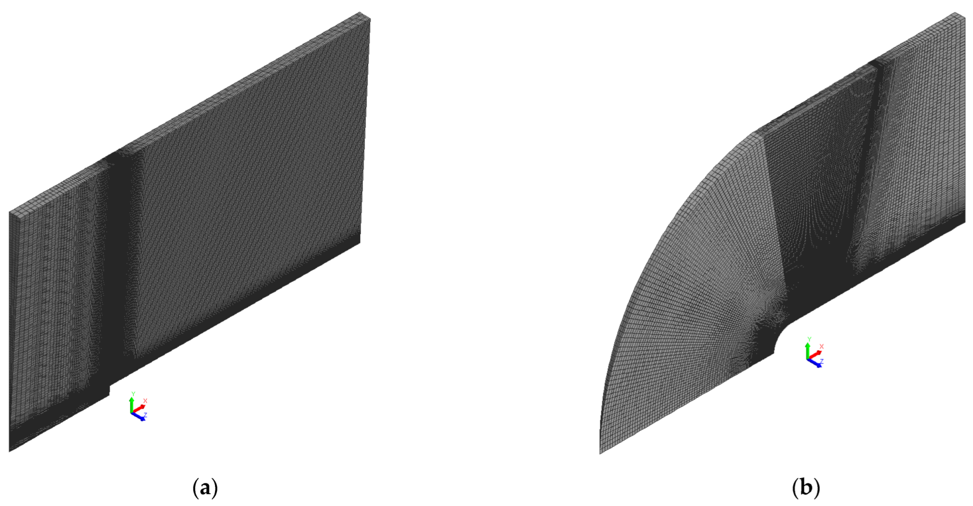
In the present study, the turbulent flow conditions with Reynolds number Re = 136,000 around a cylinder of diameter d = 0.02 m both for the plane and semispherical ends of the cylinder is considered. The characteristic features of turbulence are resolved using the SST model of linear eddy viscosity, and the SS and ZGB models of cavitation are used.

Owing to the flow symmetry, the computational domain is a sector with a 3° angle of rotation. The computational domain size excludes a strong effect of the external boundary conditions and is not less than five diameters of the cylinder in all directions beginning from the origin of coordinates.

Block-type mesh models with the mesh refinement near the body were constructed. Their general view is shown in Figure 1.

Gradually refined meshes were built to study the mesh convergence of the solution and select optimal mesh models according to

Table 1. The mesh model parameters.

Meshes with Plane End:	Nx	Ny	Nz
mesh 1	300	200	2
mesh 2	450	350	4
mesh 3	600	450	6
Meshes with semispherical end:
mesh 1	100	60	2
mesh 2	200	120	4
mesh 3	400	240	6

below.

Boundary conditions are selected in the following way: the symmetry conditions are imposed on the lateral boundaries, the input velocity of a homogeneous flow directed along the body axis is given at the input, and the pressure corresponding to the cavitation number of interest is given at the output. The symmetry condition is imposed on the upper boundary, and the cylinder surface is a no-slip rigid wall.

The commonly used physical properties of water and vapor are taken. The dynamic viscosity and density values were μ = 1.0 × 10⁻³ Pa·s, ρ = 998.2 kg/m³ for water and μ = 1.34 × 10⁻⁵ Pa·s, ρ = 0.5542 kg/m³ for vapor. The cavitation number served as an additional parameter for cavitating flows. In the problems of the flow around a body of a finite thickness, the cavitation number, σ, is defined as

$$\mathsf{\sigma }=\frac{(P-P_{sat})}{\mathsf{\rho }l{U}_{in}^2/2},$$

(17)

where P is the medium pressure; P_sat is the saturation pressure; ρ is the medium density; U_in is the inflow rate, l is a typical size. For the mesh convergence assessment problems, the cavitation number was σ = 0.3 with P = 9864 Pa and P_sat = 2736 Pa.

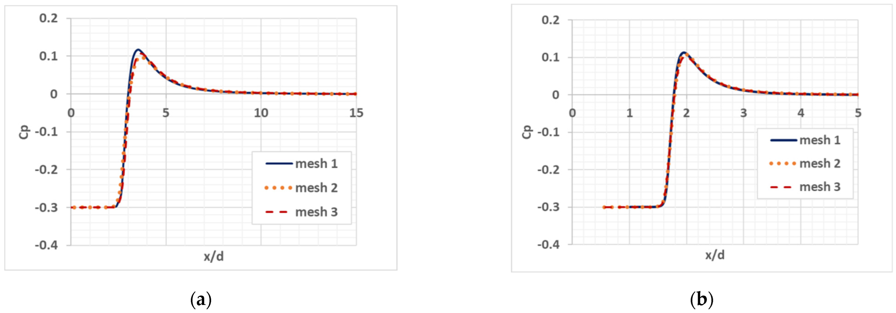
Figure 2 illustrates the results of studying the mesh convergence. The curves of the pressure coefficient vs dimensionless distance x/d are shown.

One can see from the plots above that the mesh refinement provides the solution convergence to the solution obtained on a finer mesh, while the pressure coefficient value decreases and the difference becomes noticeable in the case of the flow around the cylinder with plane end. The difference in pressure maxima between the computations on meshes 2 and 3 does not exceed 2%. In the further study, mesh 2 was used for cylinders with plane and spherical ends.

In order to estimate the cavitation area size with various cavitation numbers for flows around cylindrical bodies the SS and ZGB models of cavitation were used in computations. The following parameters were taken for the cavitation models: the number of bubbles equal to n = 10 × 10¹³ and radius of bubbles R = 10 × 10⁻⁶ m. The cavitation numbers were 0.3 and 0.5 in flows around the cylinder with plane end and 0.4 and 0.5 in flows around the cylinder with semispherical end.

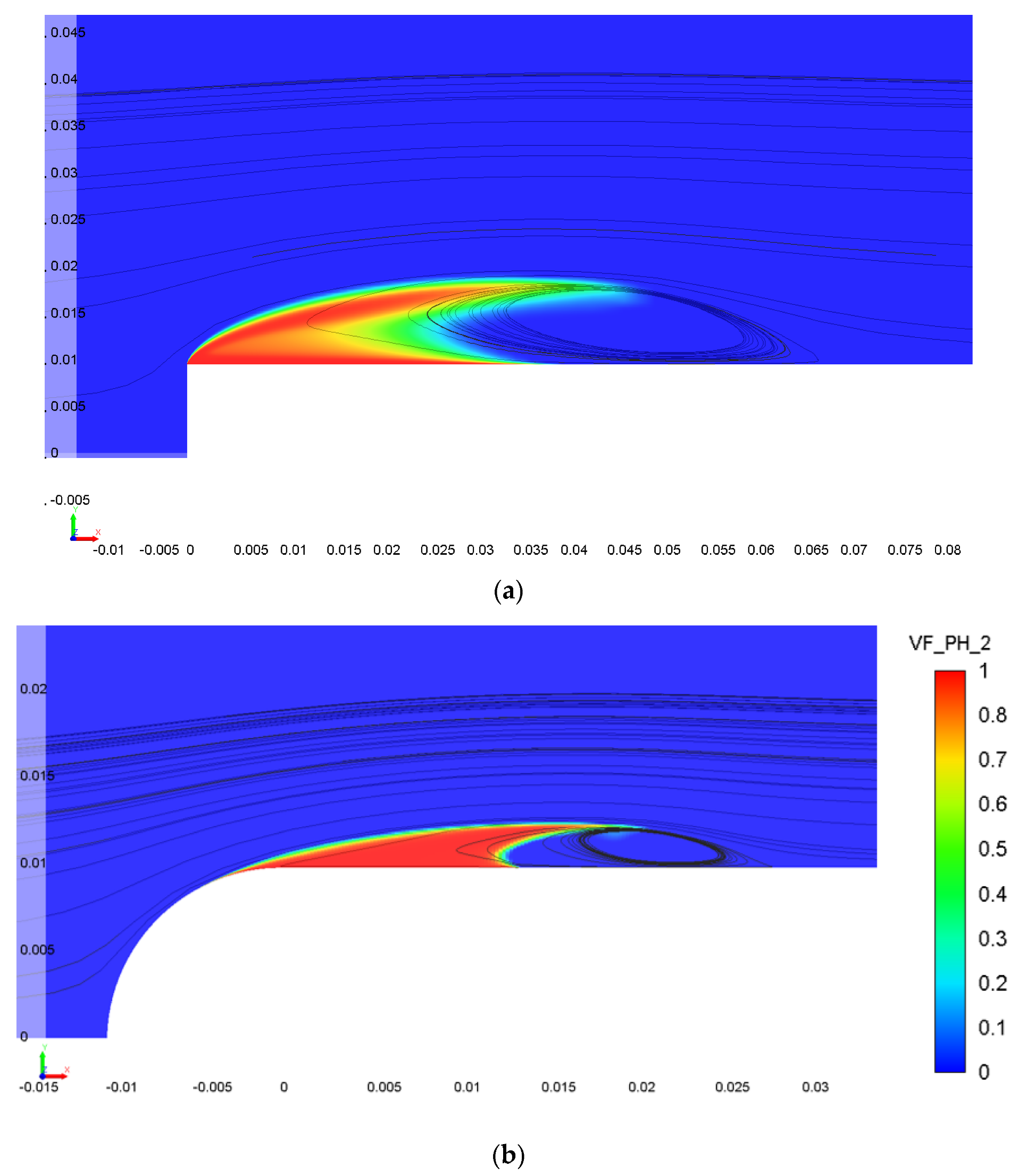
Figure 3 shows the vapor volume fraction distribution for cylindrical bodies, the cavitation number is σ = 0.3.

The cavitation cavity shapes, sizes, and lengths in flows around cylindrical bodies with various ends are very much different. For cylinders with semispherical ends the cavity size is significantly less than that for the cylinder with plane end and the flow recirculation area is observed behind the cavitation cavity. Therefore, in the case of a bluff-shaped end of the cylindrical body, the cavitating flows around such bodies have a noticeably larger cavitation area.

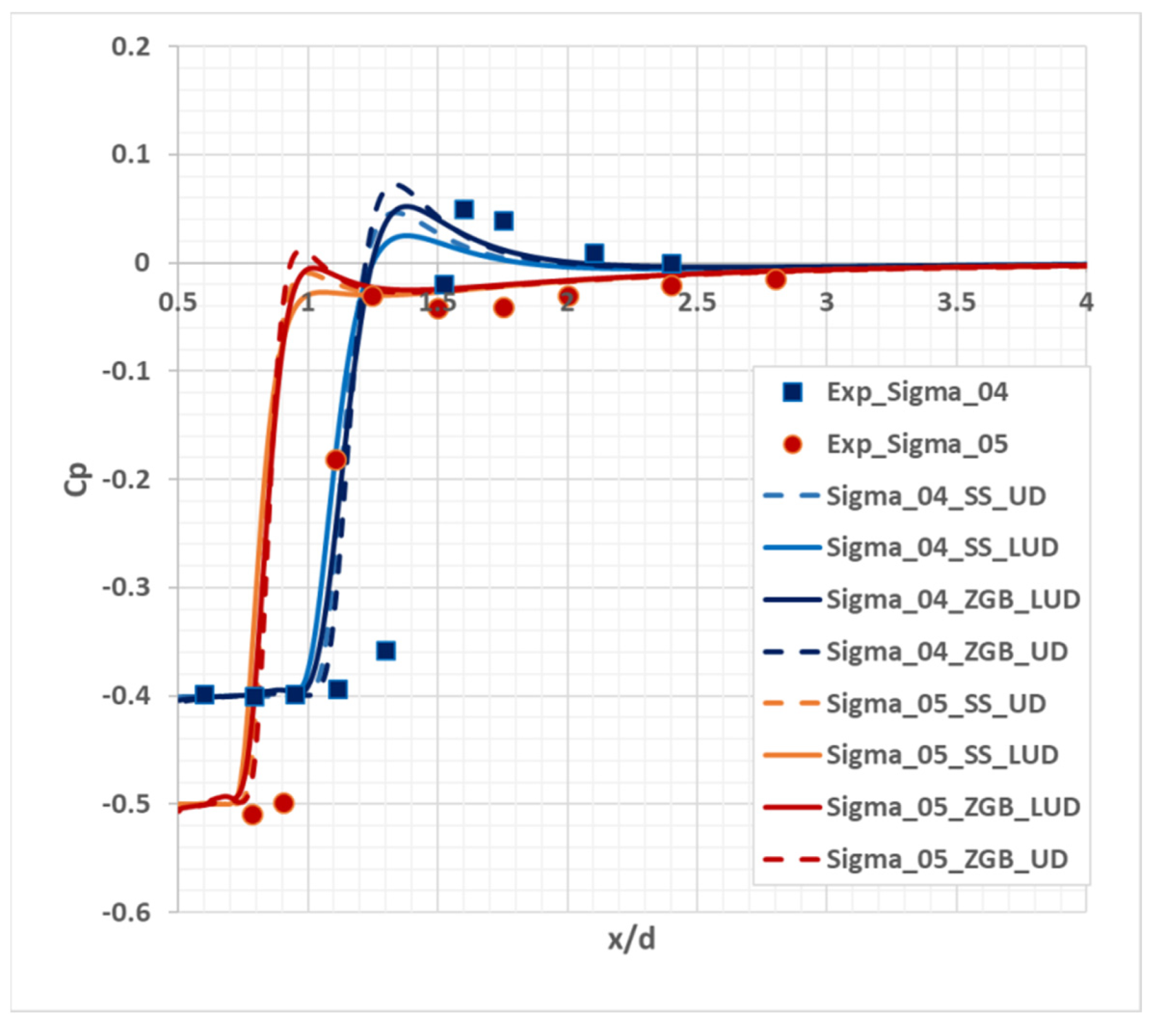
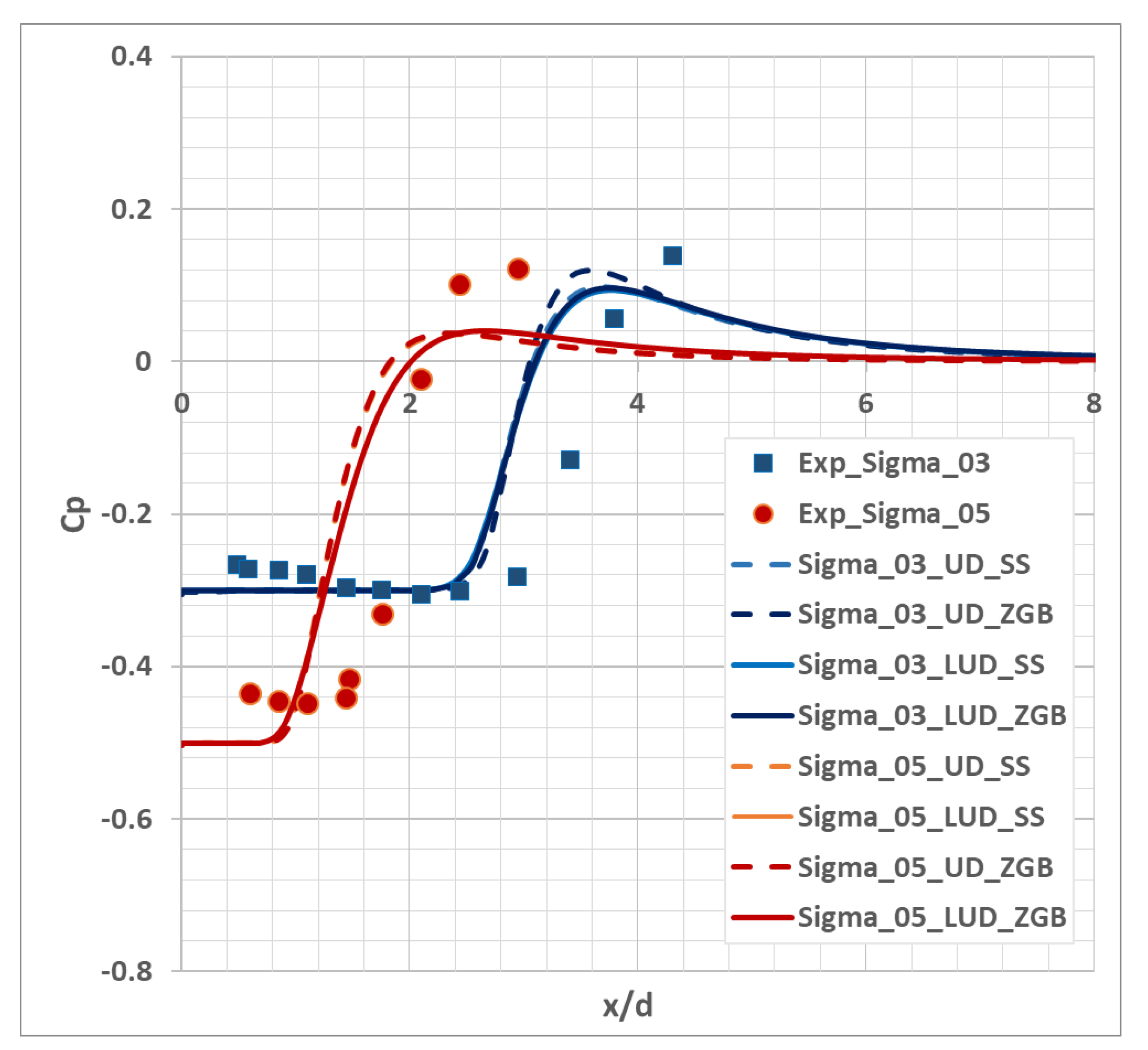
Moreover, of a particular interest is the issue of the discretization scheme effect on the pressure distribution and, consequently, the cavitation area dimensions. The figures below show the pressure coefficient distribution with different cavitation numbers for a cylinder with a semispherical end (Figure 4) and a plane end (Figure 5) in comparison with the available data of experiments. The results of using the first-order upwind scheme UD (Upwind Differences) and the second-order scheme LUD (Linear Upwind Differences) with linear interpolation [23] are compared and, also, the cavitation model effect on the pressure coefficient distribution is shown.

In the case of the flow around the cylinder with a semispherical end, the effect of both the convective flow discretization scheme and the applied cavitation model is clearly seen: the ZGB model of cavitation overestimates the pressure coefficient value with the use of the upwind scheme, while a higher order of accuracy decreases its value and, ultimately, leads to the corresponding experimental value. In the flow around the cylinder with a plane end, the significant effect of the convective flow discretization scheme is observed; as for the cylinder with a semispherical end, the LUD scheme application leads to a lower maximum of the pressure coefficient, and the results obtained with various models of cavitation are in good agreement. The simulation of flows around cylinders demonstrates the displacement of the calculated pressure coefficient profiles relative to the experimental data and, thereby, shows the underestimated dimensions of the cavitation area. The cavitation number effect is observed in the simulation of flows around cylinders with different ends. A lower cavitation number leads to a significantly larger cavitation area and this result is confirmed both numerically and experimentally.

4. Simulation of a Rotating Propeller VP 1304

To study the cavitation phenomenon, a series of cavitation tests with a VP1304 propeller in a cavitation tunnel were performed [8,24]. During these experimental investigations the cavitating flow patterns and the cavitation area positions on the blades were recorded and the propeller performance characteristics (forces, moments, and the efficiency coefficient) were found.

The problem of a steady-state uniform liquid flow around a rotating propeller VP1304 with five blades is considered. A model propeller of 0.25 m in diameter is fixed at the end of the propeller shaft.

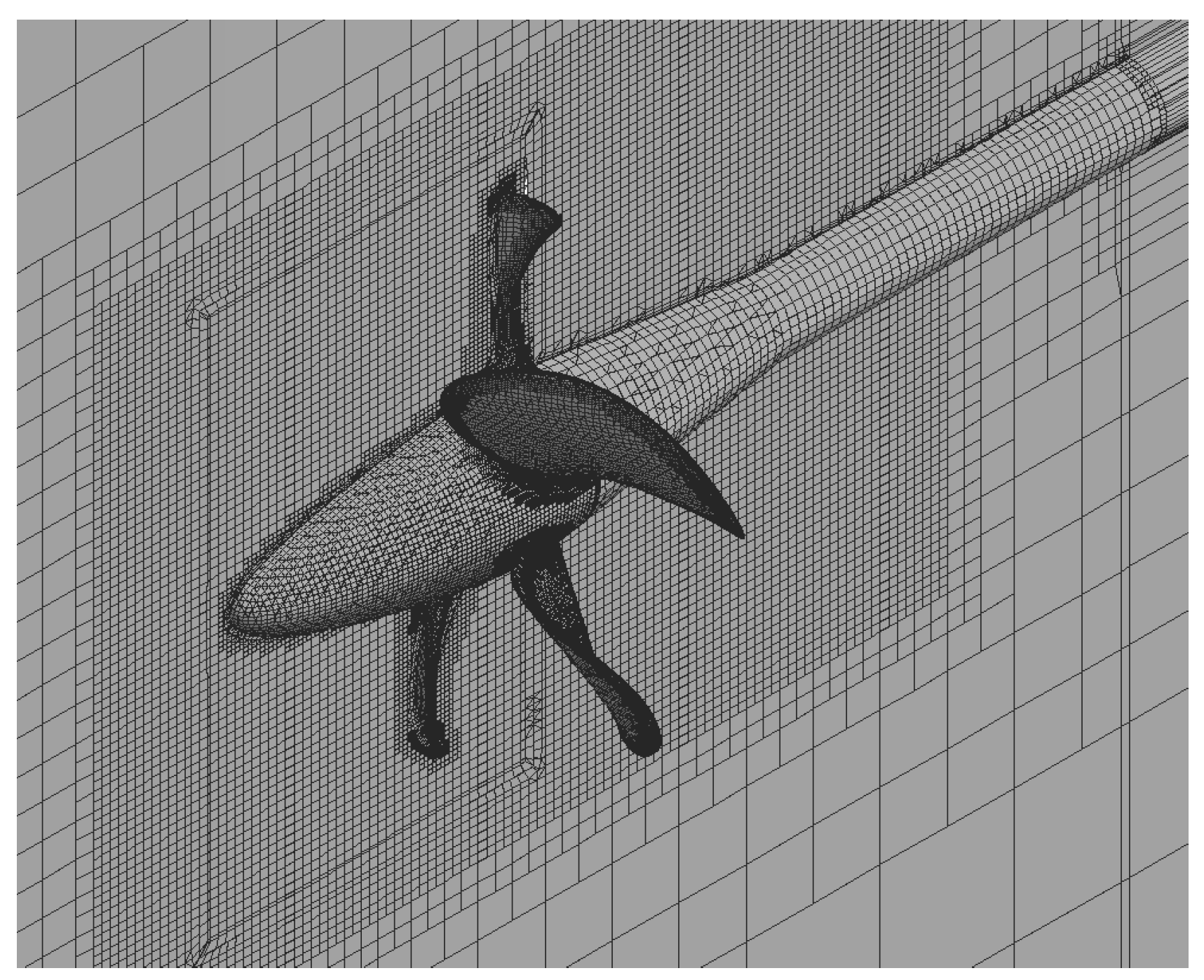
A computational mesh is generated with the cutoff method with detailing the mesh cells near the propeller blades, along the swirling flow motion direction, and in the boundary layer. The mesh model consists of two meshes generated independently of each other. The first of them is a cylindrical region around the propeller; the second mesh is a cylindrical region with the shaft on the central axis. The cell size in the rotating region is 4 × 10⁻³ m. Figure 6 shows the mesh model cross-section. The mesh includes 2.8 mln cells in total.

The propeller rotation is simulated using the interface between rotating and static regions of the computational domain. A rotating region that surrounds the propeller has the form of a cylindrical surface with the shaft as its central axis.

An incoming flow velocity is given on the input boundary and a pressure is given on the output boundary. The boundaries of the propeller are no-slip rigid walls. The symmetry condition is imposed on the lateral boundaries of the external region. The boundary condition “Interface” is imposed on the joining boundaries of the rotating and static regions.

To calculate the propeller performance curves, a series of parametric computations was carried out with the propeller rotation frequency n = 25 rev/s. The advance coefficient, J, in these computations varied within the range from 1.09 to 1.408 and was used to calculate the inflow velocity:

V_m = J·n·D_m.

(18)

The following physical properties of water and vapor were taken for these computations: dynamic viscosity μ = 0.00114 Pa·s and density ρ = 1000 kg/m³ for water; μ = 1.2676 × 10⁻⁵ Pa·s and ρ = 0.5953 kg/m³ for vapor.

For cavitating flows, the cavitation number was used as an additional governing parameter. The cavitation number, σ, is defined as (17).

The k-ω SST model of turbulence along with the laminar–turbulent transition model (Gamma Re Theta) was used to calculate the turbulent viscosity. The second-order upwind scheme LUD was used for the discretization of convective terms.

Table 2. The test modes.

Test Mode	1	2	3
Pressure in tunnel	43,071	31,353	42,603
Advance coefficient of propeller	1.09	1.269	1.408
Cavitation number	2.024	1.424	2.0

presents the parameters used in tests with cavitating flows around the VP1304 propeller. The saturated vapor pressure calculated using the water temperature was equal to 3540 Pa.

The propeller thrust and moment values were measured in these experiments and then used to calculate dimensionless characteristics, such as the thrust constant and the propeller moment, as well as the efficiency coefficient, i.e., the so called “propeller performance curves”.

The performance curves are the functions in which the thrust coefficient, moment coefficient, and efficiency of the propeller are put into correspondence to each value of the propeller advance. These coefficients are calculated according to the following formulas:

$$Kt=\frac{t}{\mathsf{\rho }{n}^2{D}_P^4},Kq=\frac{q}{\mathsf{\rho }{n}^2{D}_P^5},{\mathsf{\eta }}_0=\frac{J}{2\pi }\cdot \frac{Kt}{Kq},$$

(19)

where Kt is the thrust coefficient, Kq is the moment coefficient, η₀ is the propeller efficiency, ρ is a mean density of flow, n is the number of revolutions, and D_p is the propeller diameter.

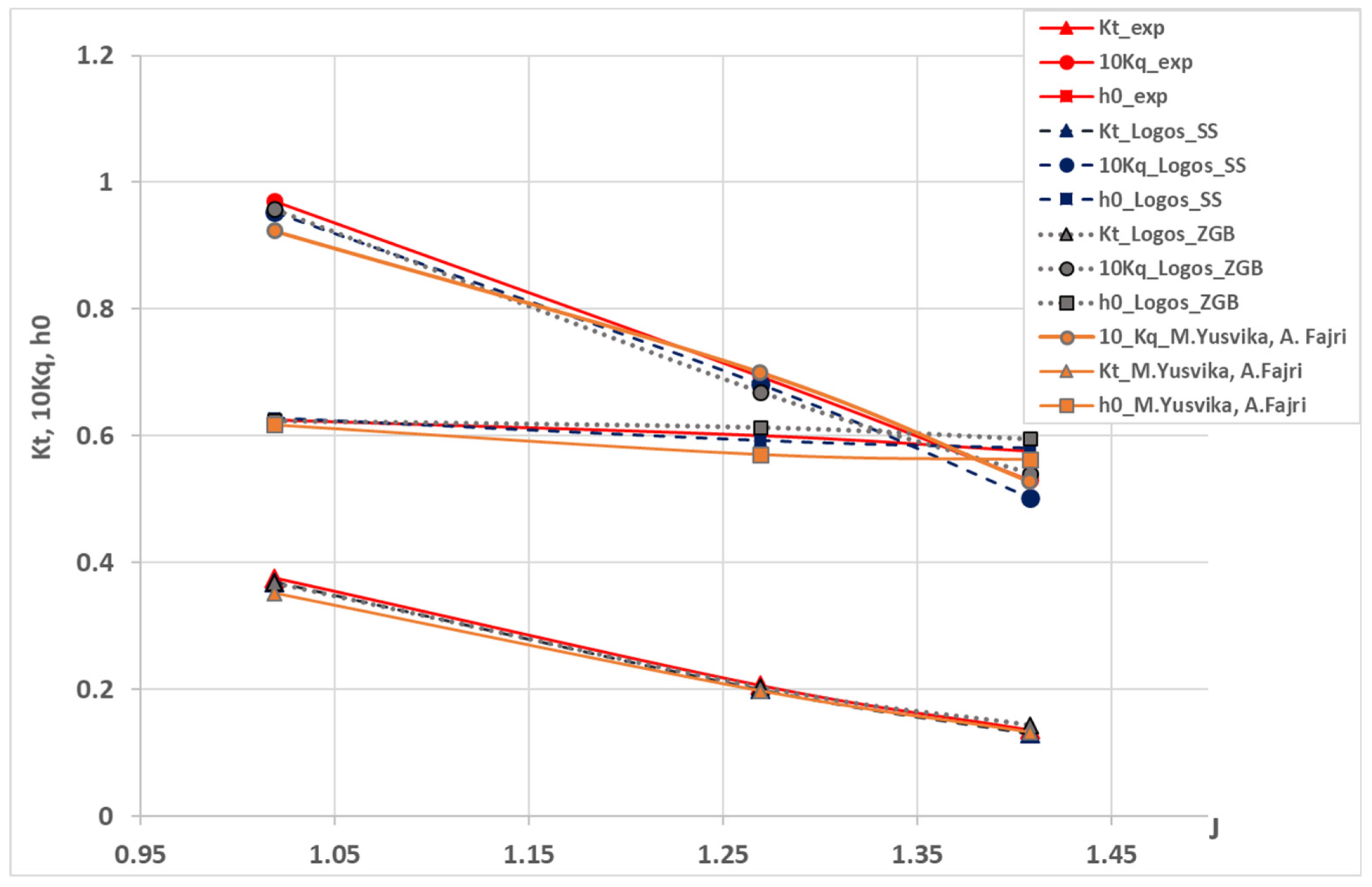
Figure 7 shows the plots of the simulation results obtained with the SS and ZGB models of cavitation. For test mode 1, the discrepancy in the values of coefficients Kq and Kt is not higher than 1.8% for both cavitation models. For test mode 2, a discrepancy maximum is observed for Kq: 5.6% for the SS model and 3.5% for the ZGB model. For test mode 3, discrepancy maxima are observed for the SS model: 5.2% for Kq and 4.4% for Kt. In the case of the ZGB model of cavitation, a maximum error was 5.3% for the thrust coefficient (Kt). The calculated Kt values for the advance coefficients close to 1 are almost the same as in experiments, while with larger values of the advance coefficient the thrust coefficient values are below the experimental ones. The numerical simulation results for the propeller VP1304 were obtained by M. Yusvika, A. Fajri, et al. [8]. The error in the calculated coefficients for the performance curves is below 6.4% with the use of the Kunz model of cavitation in combination with the SST model of turbulence. A maximum deviation is observed in the torque coefficient. The maximum deviation in the numerical simulation with the LOGOS software package does not exceed 5.6% for this coefficient.

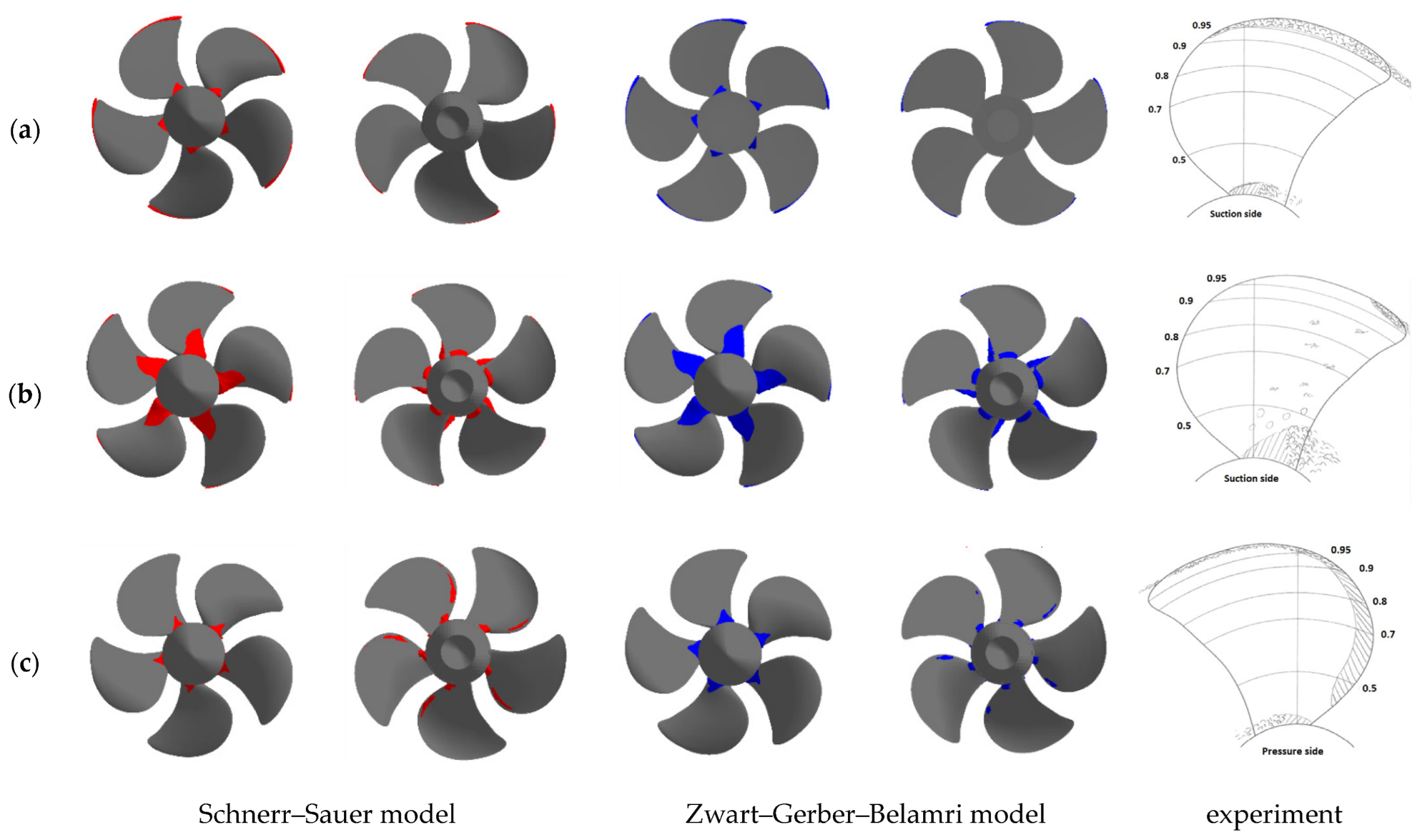
Figure 8 shows the shapes of the cavitation areas for each test mode obtained with the SS and ZGB models of cavitation in comparison with the experimentally observed patterns.

As we can see in the figures above, in all test modes the cavitation cloud shape agrees with the experimental pattern. Similarly to the experiment, for the first two modes the computation predicts the generation of the two cavitation areas: one near the propeller blade root and another along the front edge of the blade. For the second mode with a smaller cavitation number the cavitation cloud is more pronounced, both in the experiment and according to the numerical simulation results. The results of using various cavitation models agree in most cases; the cavitation cloud obtained with the ZGB model almost always has a higher volume. For test mode 3, a difference in the experimental and calculated fields is observed: when comparing the experimental pattern of cavitation vapor on the driving face of the blade with the calculated result, there is no detached flow at the blade end in computations with both the SS and ZGB models.

5. Conclusions

The paper presents a physical and mathematical model and describes the SS and ZGB models of cavitation implemented in the LOGOS software package on the basis of the VOF method. The method was validated on the test problems, for which reliable data from experiments are available. The problems of flows around cylindrical bodies with various shapes of the cylinder end and the problem of a flow around the model propeller VP1304 rotating under the developed cavitation conditions are considered. The effect of a higher-order scheme on the numerical simulation results is studied, and the SS and ZGB models of cavitation are compared. The dynamic characteristics of the propeller obtained with various models of cavitation are given in comparison with the experimental data, and the difference in their values does not exceed 5.6%. The numerical simulation with the SS and ZGB models gives similar results; however, the ZGB model allows us to obtain propeller characteristics that are in better agreement with the experimental data. The distribution fields are given for the isosurface of the vapor volume fraction for various flow conditions.