Article

A Python Toolbox for Data-Driven Aerodynamic Modeling Using Sparse Gaussian Processes

by
Hugo Valayer
1,†,‡,
Nathalie Bartoli
1,2,*,†,
Mauricio Castaño-Aguirre
1,3,
Rémi Lafage
1,2,†,
Thierry Lefebvre
1,2,†,
Andrés F. López-Lopera
3,† and
Sylvain Mouton
4
1
DTIS, ONERA, Université de Toulouse, 31000 Toulouse, France
2
Fédération ENAC ISAE-SUPAERO ONERA, Université de Toulouse, 31000 Toulouse, France
3
CERAMATHS, University Polytechnique Hauts-de-France, 59313 Valenciennes, France
4
Direction des Souffleries, ONERA, 31410 Mauzac, France
*
Author to whom correspondence should be addressed.
These authors contributed equally to this work.
Part of this work was conducted during an internship of H.V. at ONERA/DTIS.
Aerospace 2024, 11(4), 260; https://doi.org/10.3390/aerospace11040260
Submission received: 29 January 2024 / Revised: 22 March 2024 / Accepted: 25 March 2024 / Published: 27 March 2024
(This article belongs to the Special Issue Data-Driven Aerodynamic Modeling)

Abstract

:
In aerodynamics, characterizing the aerodynamic behavior of aircraft typically requires a large number of observation data points. Real experiments can generate thousands of data points with suitable accuracy, but they are time-consuming and resource-intensive. Consequently, conducting real experiments at new input configurations might be impractical. To address this challenge, data-driven surrogate models have emerged as a cost-effective and time-efficient alternative. They provide simplified mathematical representations that approximate the output of interest. Models based on Gaussian Processes (GPs) have gained popularity in aerodynamics due to their ability to provide accurate predictions and quantify uncertainty while maintaining tractable execution times. To handle large datasets, sparse approximations of GPs have been further investigated to reduce the computational complexity of exact inference. In this paper, we revisit and adapt two classic sparse methods for GPs to address the specific requirements frequently encountered in aerodynamic applications. We compare different strategies for choosing the inducing inputs, which significantly impact the complexity reduction. We formally integrate our implementations into the open-source Python toolbox SMT, enabling the use of sparse methods across the GP regression pipeline. We demonstrate the performance of our Sparse GP (SGP) developments in a comprehensive 1D analytic example as well as in a real wind tunnel application with thousands of training data points.

1. Introduction

Gathering accurate aerodynamic data to characterize the behavior of an aircraft often demands a substantial investment of time and resources. On the one hand, it calls upon aerodynamic simulations, which involve the solution of large discretized differential equations through High-Performance Computing (HPC) tools [1]. However, the use of HPC becomes expensive if a large number of simulations are required to build a comprehensive database. Despite significant advances in the past decades driven by increased computing power, simulation accuracy is still limited by issues such as turbulence modeling and discretization errors [2]. On the other hand, aerodynamic development involves real experiments, sometimes in flight but most often in Wind Tunnels (WTs). These experiments are efficient in producing thousands of observation data points with suitable accuracy [3], but are expensive to set up and come along with practical limitations. Therefore, conducting experiments at new input configurations might be infeasible. In this context, appropriate methods are needed to consider large WT datasets to leverage the information they contain fully for inference purposes.
Data-driven surrogate models offer a cost-effective and time-efficient alternative by creating a simplified mathematical representation that approximates the output of a computer code [4,5,6]. They are also valuable for approximating experimental outputs, provided they can handle random measurement errors that introduce noise into the output [7]. GPs have gained popularity in various engineering fields for constructing surrogate models, offering a flexible and probabilistic framework for modeling complex relationships in data [1,5,8]. Their ability to capture non-linear and non-parametric behavior makes them well-suited to accurately modeling aerodynamic phenomena [7,9,10,11,12]. Furthermore, GP models not only provide accurate predictions but also allow for quantifying uncertainty [13].
Despite the versatility of GPs for learning complex data, their computational complexity, which scales as O ( N 3 ) with N being the number of training points, hinders their application to large datasets. This complexity arises from the inversion of an N × N covariance matrix. Furthermore, the memory cost of storing this matrix is O ( N 2 ) . To address these limitations, sparse approximations of GPs have emerged as efficient alternatives [14,15,16,17,18]. These approaches may involve approximating the covariance matrix using a low-rank representation or approximating the posterior distribution via variational inference. Both frameworks enable scaling GPs to large datasets while preserving accurate predictions. A more detailed discussion on the computational complexity and storage of the sparse approximations used in this paper is provided in Section 2.3.
In this paper, we focus on strategies such as sparse approximation and scalable inference algorithms to mitigate computational costs and streamline the simulation time in the context of large aerodynamic databases without compromising prediction accuracy. Different strategies used to select the inducing inputs are proposed and compared in terms of computation time and accuracy. Our framework is assessed on a 1D analytic example and a real wind tunnel application with thousands of training data points. Through our comprehensive analysis, we aim to provide a holistic understanding of the trade-offs involved, allowing practitioners to make informed decisions based on their specific computational and accuracy requirements. Finally, we seamlessly integrate our open-source Python modules into the SMT toolbox [19], a versatile framework widely used in the aerodynamic field. This integration is a practical demonstration of the applicability of our framework in real-world scenarios.
This paper is organized as follows. Section 2 focuses on the definition of GPs and Sparse GPs (SGPs). Section 3 describes the features available in SMT on SGPs. Section 4 and Section 5 present numerical illustrations of our implementations on a comprehensive analytical example as well as on a real-world WT application. Finally, further discussions, conclusions, and potential future work are summarized in Section 6 and Section 7.

2. Sparse Gaussian Processes

2.1. Gaussian Processes Regression

A GP is a stochastic process, i.e., a collection of random variables (r.v’s), where any finite collection of those variables has a joint Gaussian distribution [13]. By convention, a GP { Y ( x ) ; x R d } is denoted as Y GP ( m , k ) , where m ( x ) = E ( Y ( x ) ) is the mean function and k ( x , x ) = cov ( Y ( x ) , Y ( x ) ) = E ( [ Y ( x ) m ( x ) ] [ Y ( x ) m ( x ) ] ) is the covariance function (or kernel). The operator E ( · ) denotes the expectation of r.v’s [13]. In practice, as the focus is on centered processes (i.e., m ( · ) = 0 ), statistical patterns within the data are captured by the kernel k ( x , x ) = E ( Y ( x ) Y ( x ) ) . The kernel evaluation k ( x , x ) quantifies the correlation between the r.v’s Y ( x ) and Y ( x ) . Independence between Y ( x ) and Y ( x ) implies that k ( x , x ) = 0 , while dependence implies non-zero values. For instance, a valid covariance function in dimension d can be obtained by the tensorization of the squared exponential (SE) kernel:
k ( x , x ) = σ 2 i = 1 d k ( x i , x i ) = σ 2 i = 1 d exp ( x i x i ) 2 2 i 2 ,
where σ 2 R + is a variance parameter, and i R + for i = 1 , , d , are the length-scale parameters. While σ 2 can be seen as a scale parameter of the output, i can be viewed as a scale parameter for the i-th input variable. For the kernel in Equation (1), observe that if x = x , then cov ( Y ( x ) , Y ( x ) ) : = k ( x , x ) = σ 2 , which is the maximal possible value that can be obtained. Otherwise, for distant inputs x and x , k ( x , x ) becomes smaller. We refer to [13] for other examples of valid kernels.
In GP regression, we assume that the target function f : R d R can be modeled as a realization of a (centered) GP Y. Indeed, the GP defines a probability distribution (called the prior) over possible functions that fit a set of observations ( X , y ) , where y = ( y i ) i = 1 N are noise-free observations of f at inputs X = ( x i ) i = 1 N , where N is the number of sampling points (called training points). This is achieved by the computation of the distribution of the process f ( x ) conditionally to the interpolation conditions f ( x ) = y . This conditional process, denoted here as f ( x ) | y , X , is also GP-distributed [13], i.e., f | y , X GP ( m c , k c ) . The conditional mean m c ( · ) and the conditional variance k c ( · , · ) have explicit expressions (see, e.g., [13]). While m c ( x ) is used as a point estimation of f ( x ) , the conditional variance k c ( x , x ) is used as the expected squared error of the estimate.
Here, we are interested in the case where y = ( y i ) i = 1 N are noisy observations of f at inputs X . In this case, the regression model is given by y ( x ) = f ( x ) + ε , where ε N ( 0 , η 2 ) is an independent Gaussian noise with noise variance η 2 R + . This formulation enables establishing the following distributions for the vectors f = [ f ( x 1 ) , , f ( x N ) ] and y = [ y ( x 1 ) , , y ( x N ) ] :
f | X N ( 0 , K N N ) , y | f , X N ( f , η 2 I N ) ,
where K N N = k ( X , X ) denotes the N × N matrix of covariance between all pairs of training points, and I N is the identity matrix of size N. Then, due to the Gaussian properties [13], the conditional distribution of f for a new set of N inputs X , conditionally to the dataset ( X , y ) , is also Gaussian-distributed:
f | y , X , X N K K N N + η 2 I N 1 y , K K K N N + η 2 I N 1 K ,
where K = k ( X , X ) and K = k ( X , X ) . The distribution in Equation (3) is called the posterior distribution and is used for regression purposes in the same manner as explained for the noise-free case.

2.2. Covariance Parameter Estimation

The accuracy of predictions hinges on how well the GP fits the regression model y. Therefore, the choice of the kernel and its parameters is key. In practice, the kernel k is generally assumed to belong to a parametric set of covariance functions (see, e.g., Equation (1)) with parameters Θ R p , with p being the number of kernel parameters. Then, a better fitting of the GP relies on the proper estimation of a set of parameters θ Θ , for instance, for the kernel in Equation (1), and for the noisy case, θ = ( σ 2 , 1 , , d , η 2 ) . This step is typically achieved by minimizing the Negative Marginal Log Likelihood NMLL : = log p θ ( y ) , which is given by the negative log of the Gaussian probability density distribution (pdf):
NMLL = N 2 log ( 2 π ) + 1 2 log det K N N + η 2 I N + 1 2 y K N N + η 2 I N 1 y .
By minimizing the NMLL, we are looking for a model (i.e., the set of parameters θ ) that maximizes the pdf p θ ( y ) . This leads to a better fit of the data. It is worth clarifying that considering the kernel in Equation (1), the covariance matrix K N N is then parameterized by ( σ 2 , 1 , , d ) . This dependence is not explicitly indicated in Equation (4), nor in subsequent formulas, for the sake of simplicity in notation. Note from Equations (3) and (4) that the complexity of the GP relies on the inversion ( O ( N 3 ) ) and storage ( O ( N 2 ) ) of the covariance matrix K N N . This computation poses significant challenges, particularly when dealing with large datasets. To mitigate this drawback, sparse approximations of GPs have been introduced in prior studies such as [14,15,16,17].

2.3. Sparse Approximations of Gaussian Processes

The key idea of sparse approaches is to select a set of inputs Z = ( z i ) i = 1 M known as inducing inputs, and its corresponding (noisy) output set u = ( u i ) i = 1 M known as inducing variables. The introduction of the inducing points allows the approximation of the exact GP by exploiting the structure of the covariance matrix. Here, we focus on the Fully Independent Training Conditional (FITC) [15] and Variational Free Energy (VFE) [16] methods.

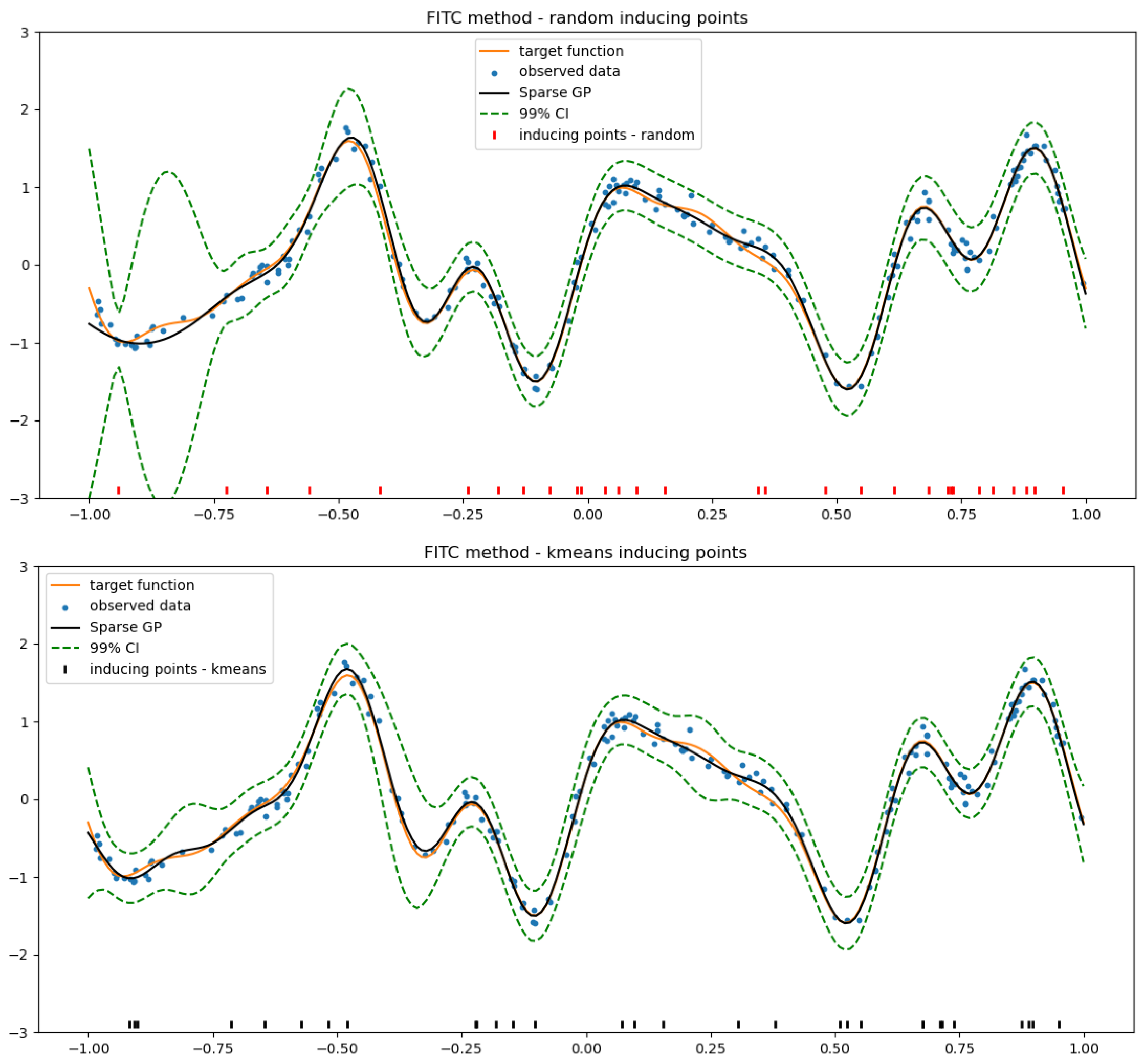
2.3.1. Fully Independent Training Conditional (FITC)

The FITC method relies on a Nyström (low-rank) approximation of the kernel matrix K N N , which introduces the following modified kernel matrix:
Q N N = K M N K M M 1 K M N ,
where K M M = k ( Z , Z ) is the covariance matrix between all pairs of inducing inputs Z , Z , and K M N = k ( Z , X ) is the covariance matrix between all pairs of inputs and inducing inputs. In the FITC, an additional term is considered, seeking to correct the diagonal of the covariance matrix. For noisy observations, the covariance matrix K N N + η 2 I N is approximated by the following:
K F I T C = Q N N + diag K N N Q N N + η 2 I N .
The kernel parameters of the approximated GP can be estimated by minimizing the NMLL in Equation (4). The inversion of Equation (5) can be performed more efficiently through the application of the matrix inversion lemma ([13], Appendix A.1), resulting in a significant gain in terms of the computational cost, from O ( N 3 ) to O ( N M 2 ) . While the optimization of the new approximated NMLL is tractable, it may not consistently approximate the exact GP. This lack of reliability stems from the absence of any guarantee that the distribution of the approximated GP closely matches that of the exact one.

2.3.2. Variational Free Energy (VFE)

The VFE method focuses on minimizing the Kullback–Leibler (KL) divergence between the exact GP posterior p ( f , u | y ) and a variational distribution q ( f , u ) . The minimization of the KL divergence is equivalent to maximizing the Evidence Lower Bound (ELBO) [20]:
ELBO log p f , u , y q f , u q f , u d f d u = E f , u q f , u log p f , u , y q f , u ,
where E f , u q f , u is the expectation of ( f , u ) with respect to q f , u . It has been shown in [16] that an optimal distribution for q ( u ) can be achieved, and that the NMLL for hyperparameter learning is given by the following:
NMLL V F E = N 2 log ( 2 π ) + 1 2 log ( | K V F E | ) + 1 2 y K V F E 1 y + 1 2 η 2 tr ( K N N Q N N ) ,
where K V F E = Q N N + η 2 I N . Unlike FITC, the diagonal correcting term is no longer needed.
Independently of the sparse approach, the choice of M must seek a trade-off between computational complexity and prediction accuracy. While SGP implementations offer faster computations for M N compared to exact GP inference, the accuracy of predictions tends to be lower [17,18]. In practice, M is often fixed to be large enough to ensure accurate predictions while maintaining tractable CPU times. However, the specific value of M may vary depending on the specifications of the machine used for the experimental setup.

2.3.3. Comparison and Contrast of the Two Methods

An analysis of both methods was performed by [21]. Their experiments showed that the FITC method tends to overestimate the marginal likelihood and underestimate the noise variance parameter, often being incapable of recovering the true posterior. By contrast, the VFE method seems to overestimate the noise variance but correctly identifies the true posterior. The main advantage of the VFE is that the NMLL V F E is a true bound on the NMLL. However, as illustrated in Section 4 and Section 5, the performance of each method depends on the target function and on the choices made for initialization and optimization.

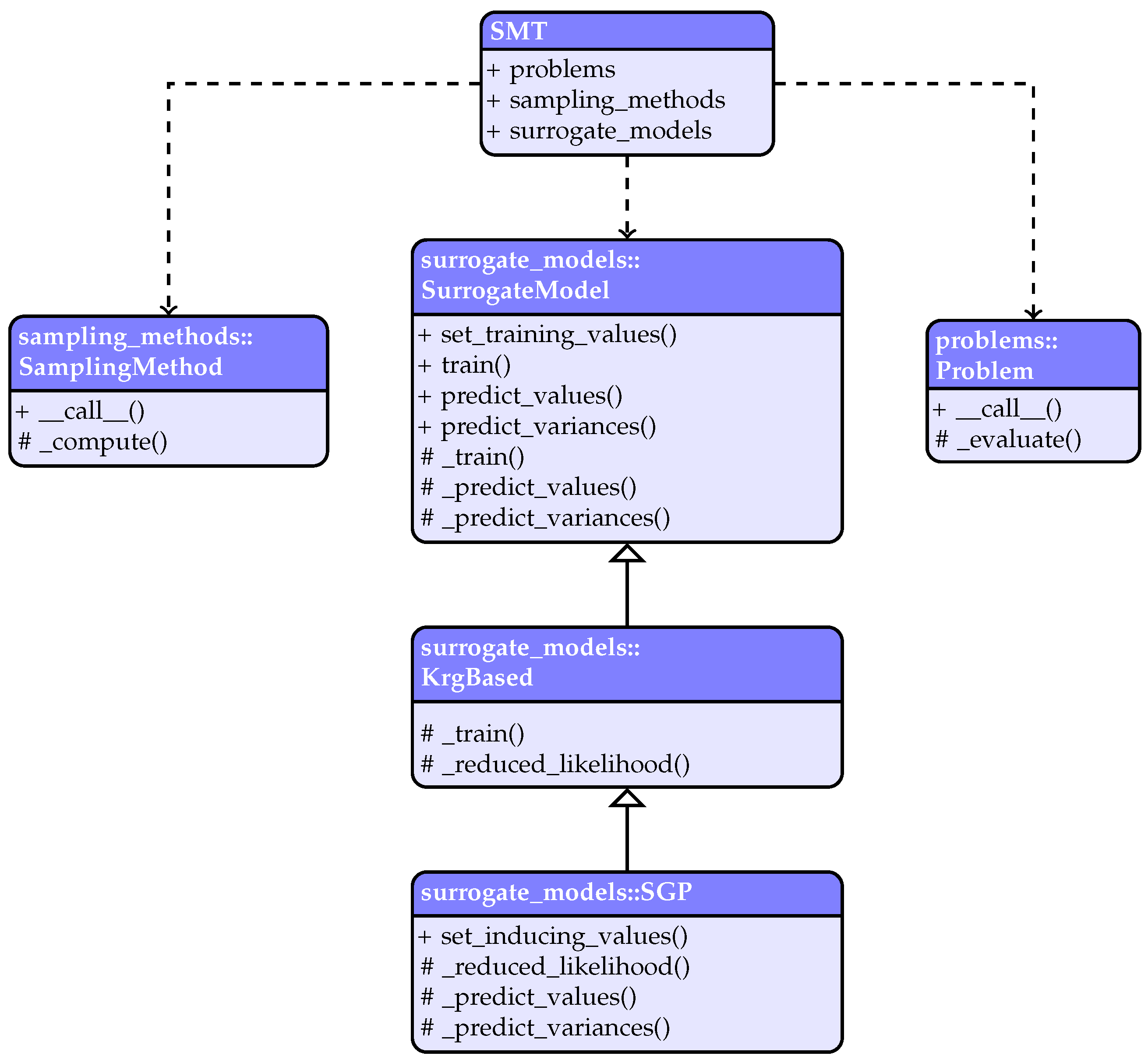
3. Surrogate Modeling Toolbox (SMT)

SMT stands as a robust tool for surrogate modeling, optimization, and sensitivity analysis, offering a comprehensive set of features tailored for constructing data-driven models and leveraging them in various engineering applications [19,22]. With a user-friendly interface and online documentation, SMT aims to streamline the application of surrogate models in practical scenarios, making it accessible to practitioners. In addition, new surrogate models can be developed and integrated. SMT comprises three main sub-modules: sampling_methods, surrogate_models and problems, each dedicated to implementing a range of sampling techniques, surrogate modeling techniques, and benchmarking functions, respectively. Each sub-module has a well-defined API that has to be defined for a given algorithm by a specific sub-class. In the case of sparse GPs, the SGP class inherits from the GP-based surrogate class (named KrgBased, from Kriging), while taking into account both the FITC and VFE inference. We refer to Appendix A.1 for further details regarding the numerical implementations of these methods.
The implementation of the FITC and VFE methods in SMT 2.3 draws inspiration from existing ones in the GPy [23] and GPflow [24] toolboxes, particularly regarding the matrix computation techniques used to achieve efficient implementations. However, it should be pointed out that, concerning the model training process, optimization of the ( z i ) i = 1 M locations of the inducing inputs is still unavailable, unlike in other libraries. In addition, sparse methods in SMT do not account for a mean function, i.e., the trend of the SGP is equal to zero. These choices are not necessarily restrictive, as a smart initialization of the inducing inputs typically yields satisfactory results (see the experiments in Section 4 and Section 5). Figure 1 illustrates the design of SMT 2.3 relevant to SGPs. After setting the training data ( x i , y i ) i = 1 N (a common feature across all surrogates), the set of inducing inputs ( z i ) i = 1 M required by the sparse algorithms can be randomly picked from the training dataset or specified using the set_inducing_points() method. The train() method from the KrgBased class maximizes the NMLL, provided for the SGP class, and returns the optimal hyperparameters using the prediction features: _predict_values() and _predict_variances().

4. Numerical Illustrations

Here, we evaluate the performance of the FITC and VFE methods when applied to an analytical test case, providing a comparative analysis of the results. We also discuss the available strategies to improve the results and reduce the computation time associated with the optimization step. Source codes of SMT 2.3 are available in the Github repository: https://github.com/SMTorg/smt (accessed on 10 January 2024). The numerical illustrations presented in this section are publicly available in the Github repository: https://github.com/SMTorg/smt-sgp-paper (accessed on 10 January 2024). All results were obtained using an Dell Intel® i7 CPU 10850H @ 2.70 GHz core and 32 GB of memory.

4.1. Analytical Example Database

We considered the 1D benchmark function suggested by the GPflow toolbox [24] (source: https://gpflow.readthedocs.io/en/v1.5.1-docs/notebooks/advanced/gps_for_big_data.html, accessed on 10 January 2024):
f ( x ) = sin ( 3 π x ) + 0.3 cos ( 9 π x ) + 0.5 sin ( 7 π x ) ,
for x [ 1 , 1 ] . We generated the training set of inputs X = ( x i ) i = 1 N , called the Design Of Experiments (DoE), by sampling N = 200 values from a uniform distribution U ( 1 , 1 ) . We then evaluated f at inputs X , and introduced Gaussian noise with the variance η 2 = 10 2 . Figure 2 illustrates the 1D function and the generated training dataset.

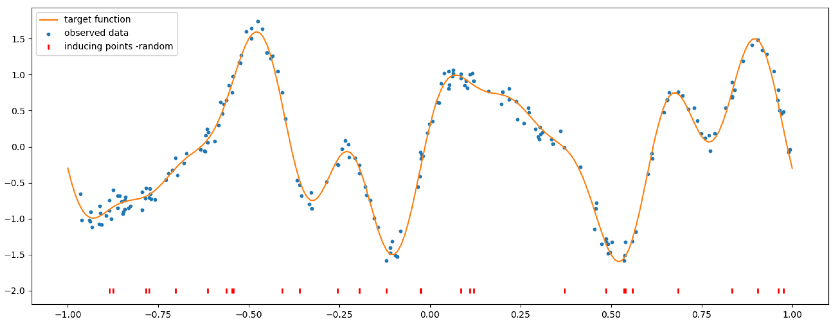
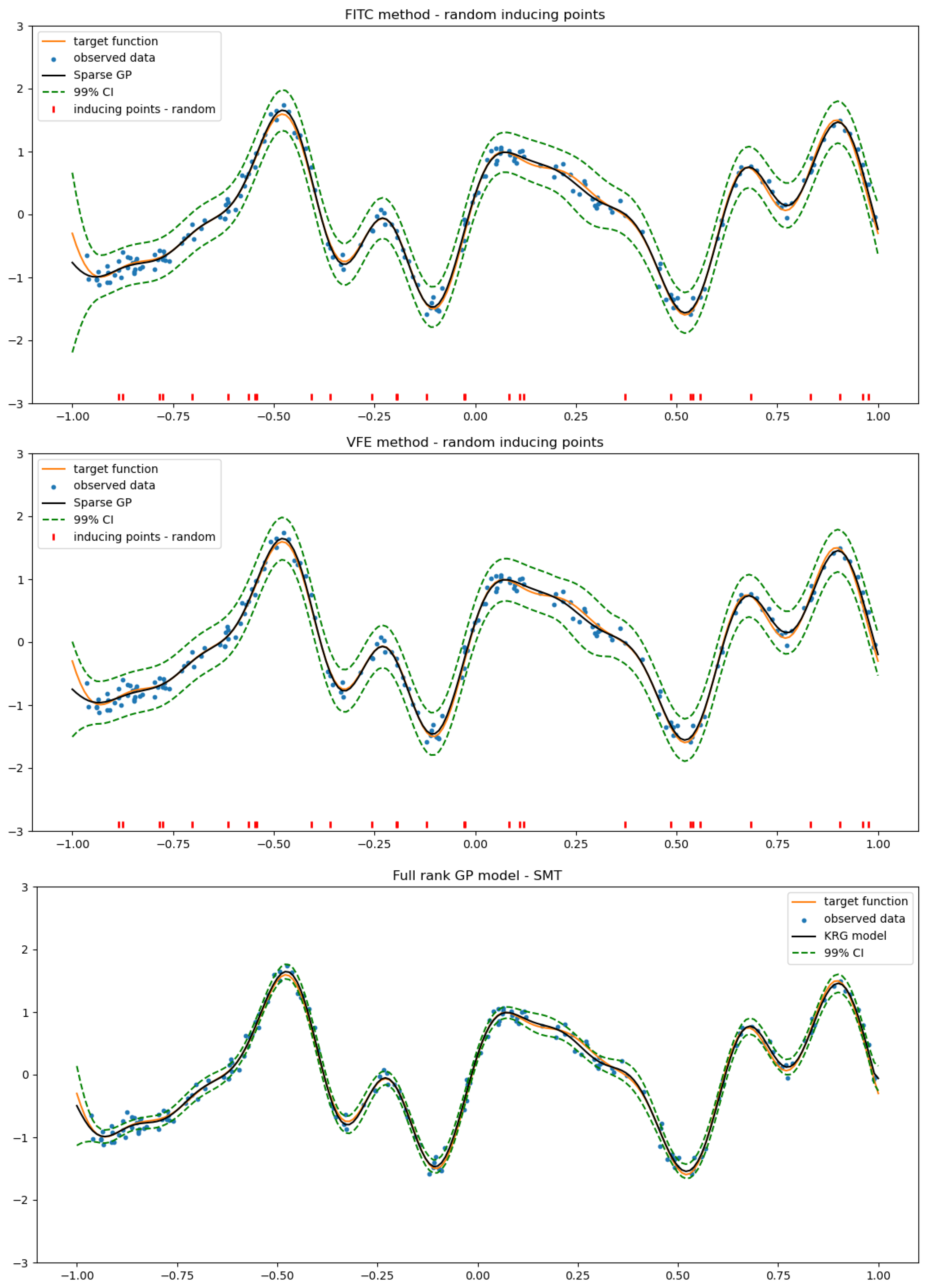
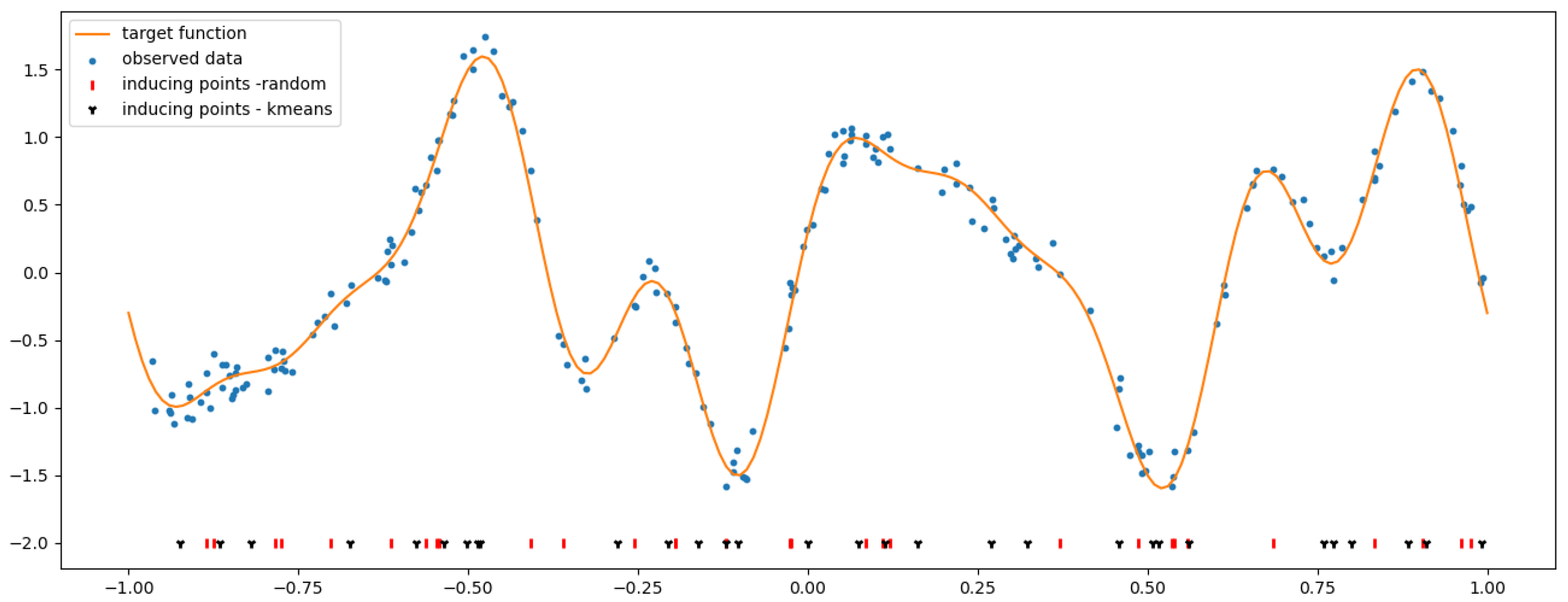
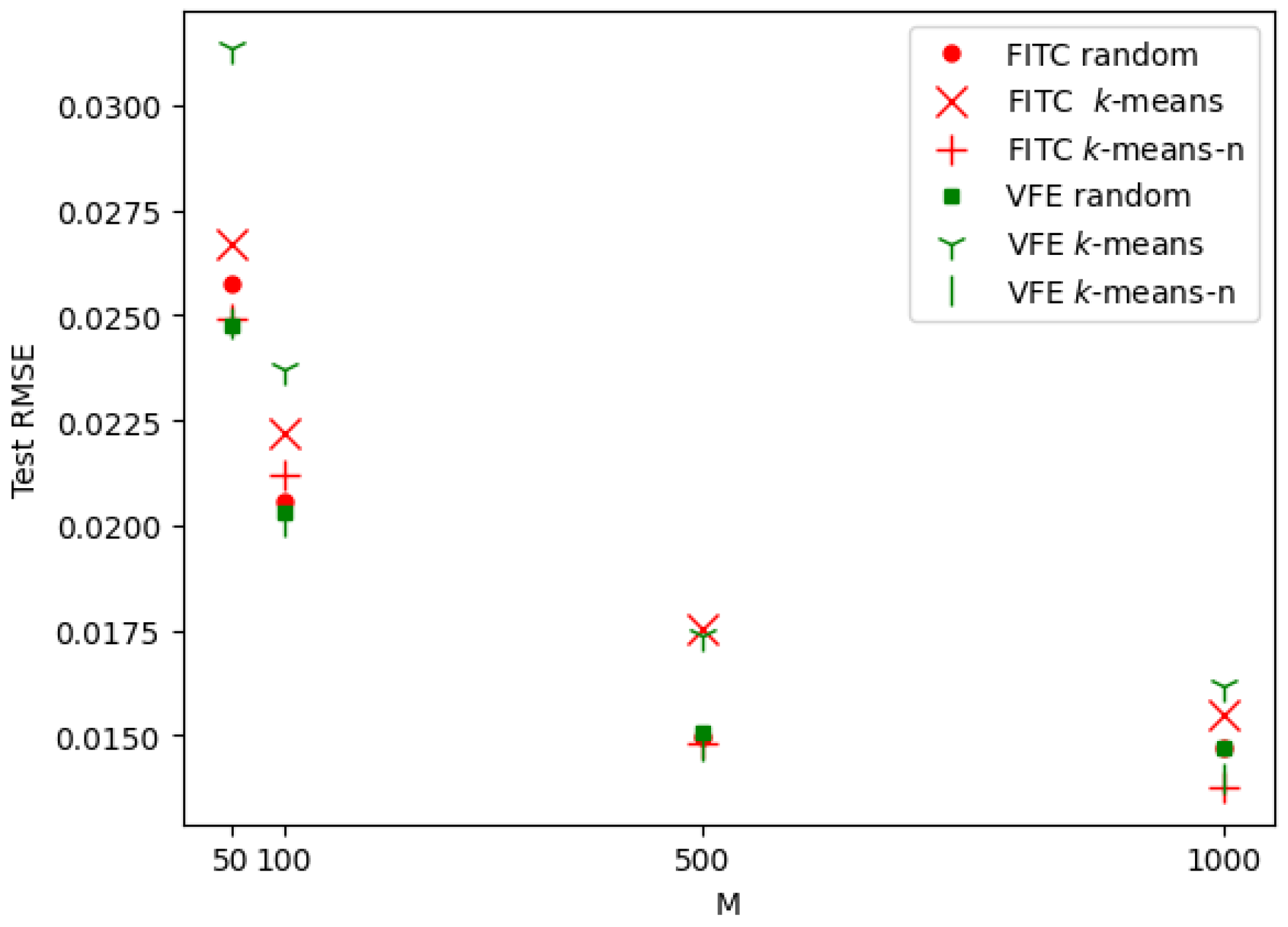
4.2. SGP Using a Random Selection of Inducing Inputs

Using the noisy training data generated in Section 4.1, we proceeded to define the SGP model. We first needed to define the inducing inputs Z = ( z i ) i = 1 M . By default, if they are not specified before proceeding to the model-training stage, SMT randomly selects them from the dataset, as illustrated in Figure 2.
Figure 3 shows the predictions obtained by SGPs using both the FITC and VFE, and by an exact GP. Both models have been defined with the default parameters of the SMT toolbox (square exponential kernel, predefined initial values, and bounds for the kernel parameters ( σ 2 , θ ) and the noise variance η 2 ), and trained via maximum likelihood. The SGPs were built with M = 30 random inducing points. From Figure 3, we can observe that while the three models provided similar predictions, the confidence intervals for the SGPs tended to be overestimated. This phenomenon is well known in the SGP literature and is a consequence of the sparse approximation when considering M N  [17,18]. The predictive confidence intervals of the SGPs became thinner as M increased, and converged to those of the exact GP when the inducing inputs Z exactly coincided with the training inputs X .
Table 1 presents a comparison of the optimal values of the GP parameters ( σ 2 , θ , η ) and the likelihood, training time, and RMSE errors for the three GP-based models discussed in Figure 3. The RMSE criterion is computed by the following:
RMSE = i = 1 N t ( y ( x i ) y ^ ( x i ) ) 2 N t ,
where N t is the number of data points, i = 1 , , N t , y ( x i ) is the true value at point x i , and y ^ ( x i ) is the associated predicted value. The RMSE is computed on the training and test sets. For the test set, we considered N t = 10 3 random input values. The results in Table 1 evidence that the SGPs were twice as fast as the exact GP and that they led to RMSE values of the same order, endorsing the practical advantage of the former models.
To further illustrate the computational benefit of SGPs in inference purposes, Figure 4 shows the training time for the exact GP and SGP-FITC as a function of the number of training points N for our analytical example. The trend of both profiles confirms that the inference for the SGP-FITC scales linearly as O ( N M ) , whereas that of the exact GP scales quadratically as O ( N 2 ) . Moreover, it is observed that the computational gains achieved with the SGP become more substantial for datasets containing more than 10 3 training points. This computational advantage will be key in the aerodynamic application discussed in Section 5, where the dataset comprises tens of thousands of data points.

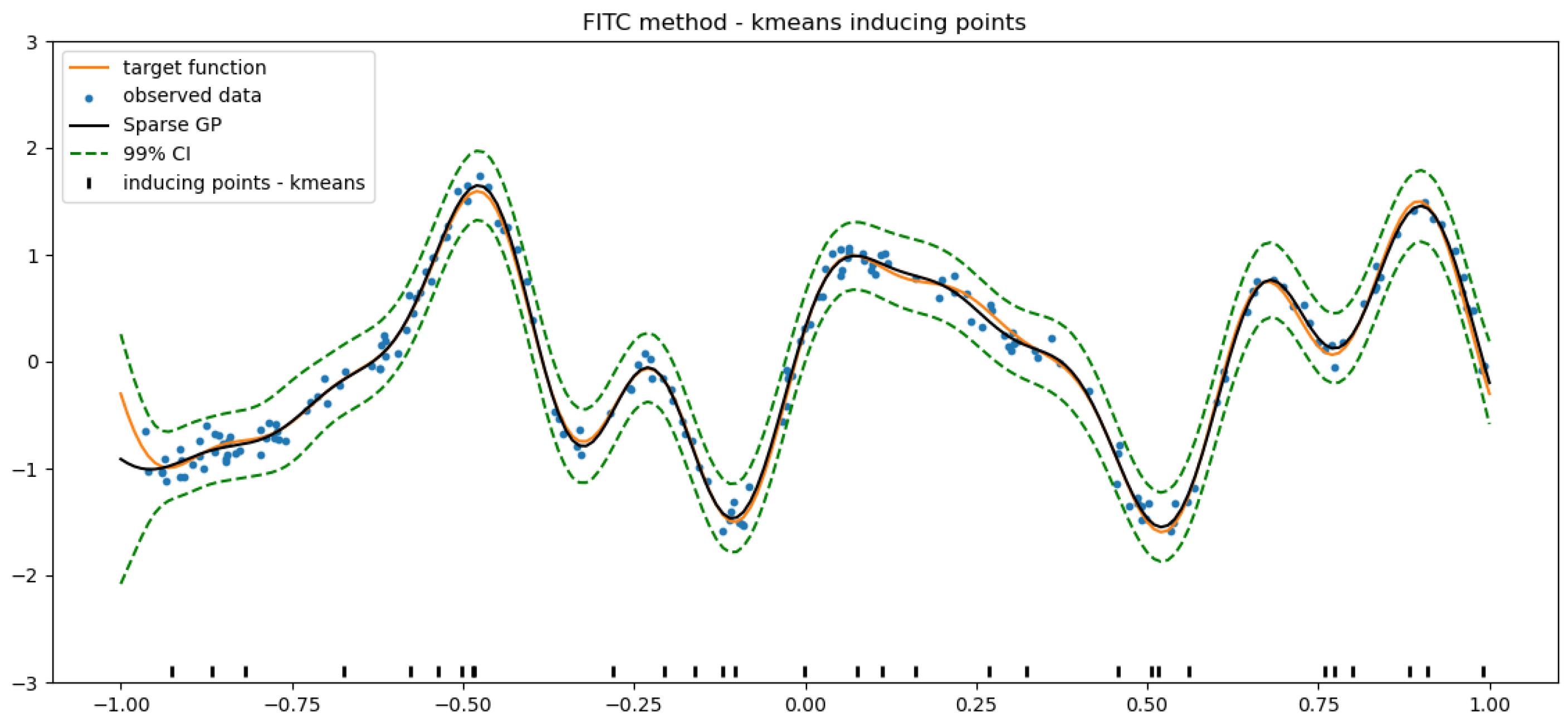
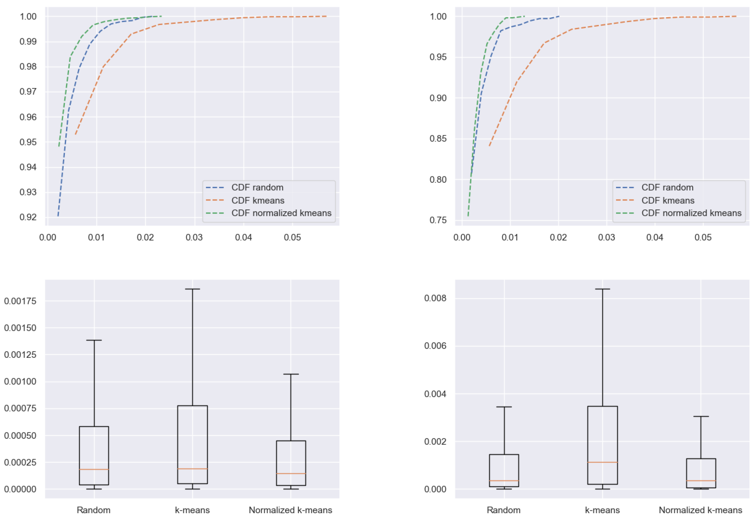
4.3. k-Means Clustering for the Selection of Inducing Inputs

As previously mentioned in Section 3, the current implementation of SGPs within SMT does not optimize the location of the inducing inputs Z . In SMT, these inputs are either randomly selected from the training set or directly defined by the user. However, this choice can significantly impact the inference accuracy, as the inducing inputs can be considered as “representatives” of the entire training set.
An appropriate selection of inducing inputs would ideally balance the coverage of the data points with a local focus on areas with high variations, such as discontinuities or humps. A random selection among the training points may lead to poor results if they are scarce in a certain region of the input space (see Figure A1). To mitigate this issue, clustering methods such as k-means have been considered to initialize the inducing inputs [25].
As discussed in Section 2.3, the number of inducing inputs M (i.e., clusters) is often known due to the limitations of the machine used for the experimental setup. Therefore, the consideration of more advanced but resource-demanding non-parametric clustering methods is not necessary in practice. For instance, the experiments in this section have also been conducted using the DBSCAN approach in [26]; however, the results were outperformed by k-means in terms of the RMSE. In particular, DBSCAN has focused the selection of inducing inputs mainly in regions with high concentrations of data. This resulted in uncovered high-variability regions with few data points, for instance around x = 0.6 , 0.2 , 0.65 , consequently leading to a decrease in the accuracy of the predictions. Therefore, in the following, we have decided to focus on k-means due to its simplicity and efficiency.
Here, to obtain a smart positioning of the inducing points without requiring an optimization step, we propose to proceed as follows:
  • Perform k-means clustering on all input–output pairs of the observations ( X , y ) to partition the training set into M clusters ( S i ) i = 1 N , each one being characterized by its centroid μ i = ( x ˜ i , y ˜ i ) .
  • Define the inducing inputs as the x-component of the centroids μ i , i.e., Z = ( x ˜ i ) i = 1 M .
Contrarily to the random scheme, setting Z by applying k-means clustering on input–output data pairs promotes the allocation of inducing inputs while taking into account the distribution of data points (see, e.g., Figure 5). Note, that unlike the choice by random permutations, the induced inputs defined by the k-means-based algorithm no longer need to be existing points in the dataset.
As shown in Figure 3, the random approach leads to an uncovered area around x = 0.25 , which explains the high predicted variance of the model in this region. Figure 5 shows that the inducing inputs are placed taking into account the distribution of input variables x while concentrating points in regions with a high variability of the output (e.g., around x = 0.5 , 0.25 , 0.5 ). Unlike the random scheme, k-means has also added inducing points around x = 0.25 . From Figure 6, it can be noted that the SGP with the k-means-configuration of inducing points leads to more accurate confidence intervals, in particular around x = 0.25 .
The results in Table 2 show that, compared to Table 1, the k-means-based scheme leads to slight improvements in both the likelihood and RMSE. These improvements are more noteworthy, as the random scheme fails to promote coverage of data points. An example where the random scheme can severely degrade the SGP accuracy is provided in Appendix A.2.1.

5. Wind Tunnel Application

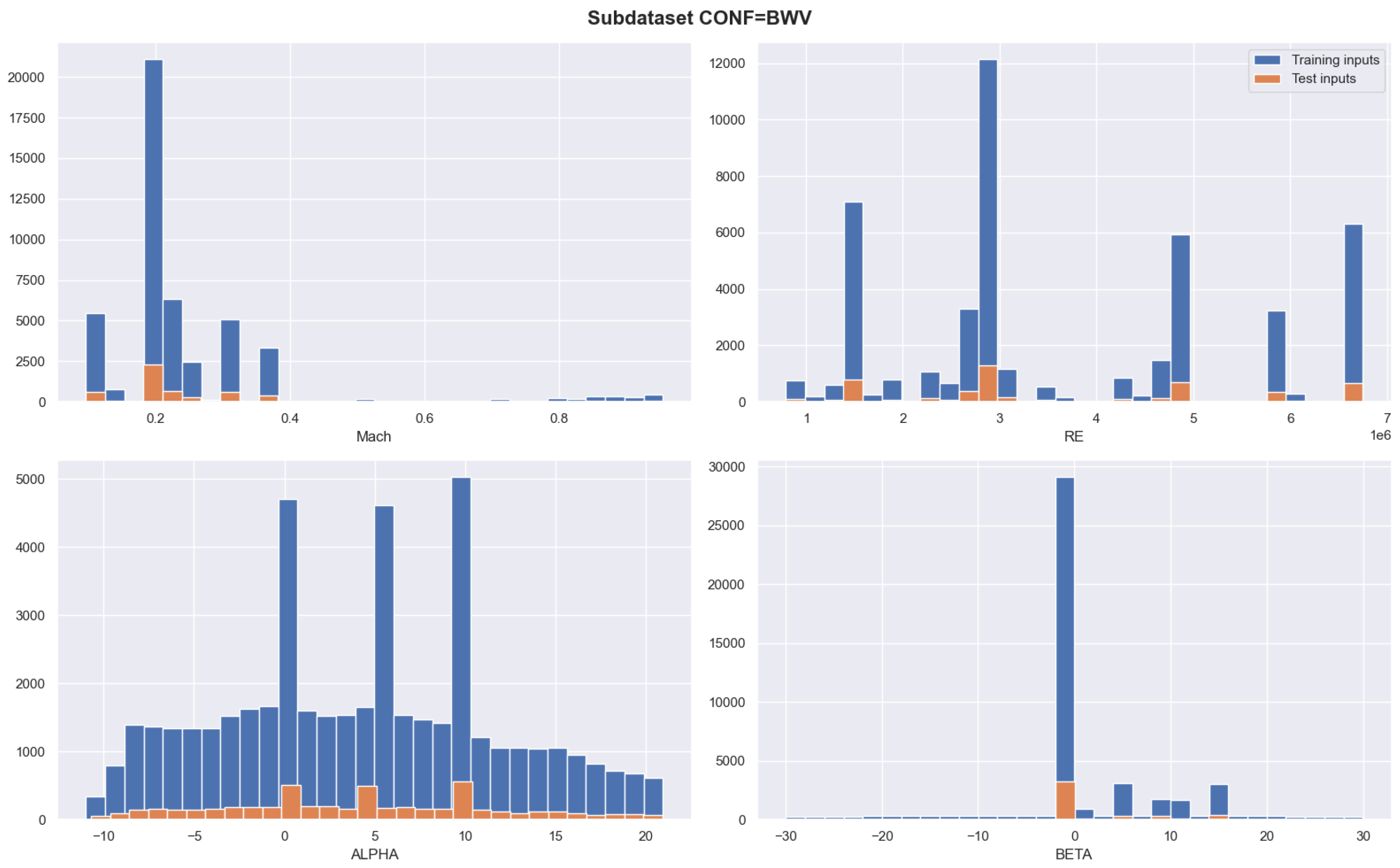
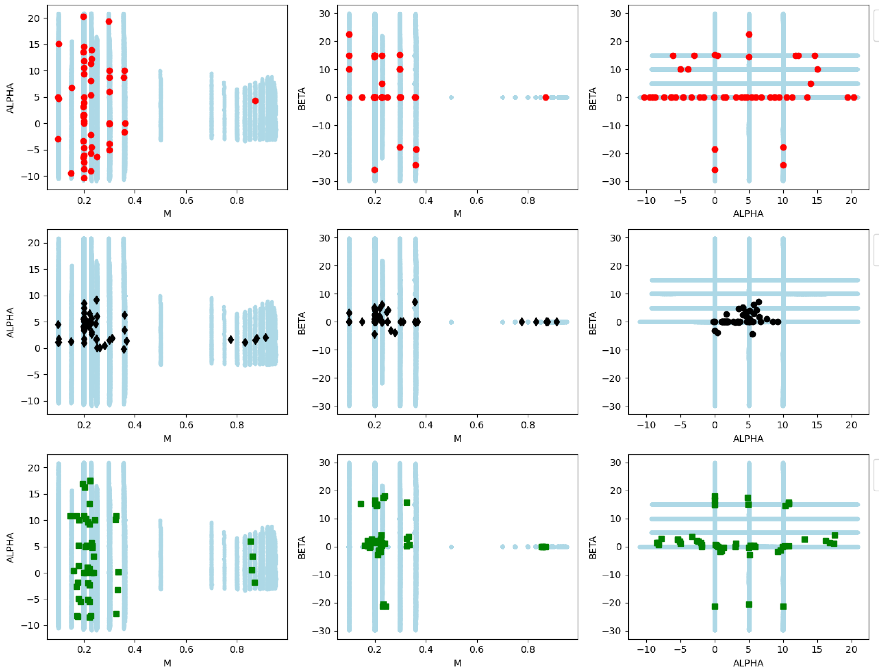
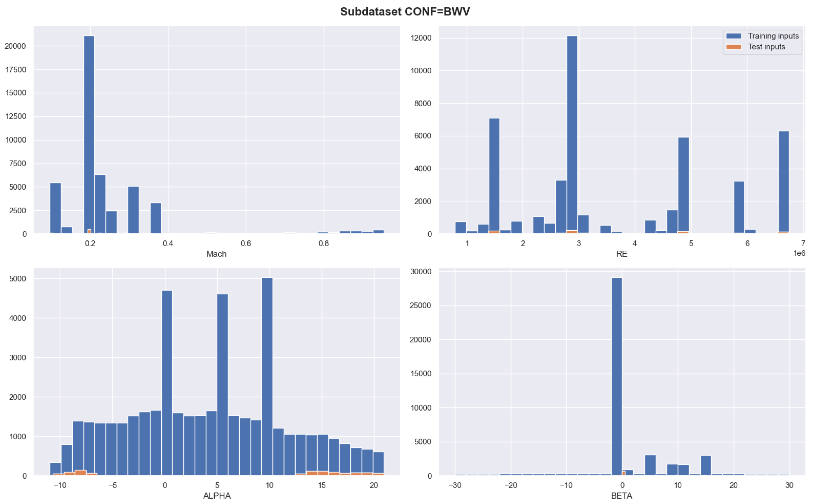
5.1. Database Description

The Wind Tunnel (WT) database used in this study is derived from the NASA Common Reference Model (CRM) [27]. Experimental testing has been conducted at ONERA’s WT department encompassing two ONERA WT facilities: F1-WT, in Fauga, which focuses on high Reynolds values and Mach numbers ranging from 0.05 to 0.36 [28]; and S1-WT, in Modane, which focuses on transonic speeds [29]. The CRM shape was used to build two Large Reference Models (LRM): the first one for S1-WT with a wing span of 3.5 m (scale 1/16.835) and the second one for F1-WT with a wing span of 3 m (scale 1/19.5). Aeroelastic deformations were considered in the design to produce a shape under load that is comparable to previous CRM tests in NTF [30] and ETW [31]. The WT models were equipped with hundreds of pressure taps, but for the present study only the aerodynamic forces measured by internal balances are considered. The measurements were corrected from the effect of the WT walls [32], and they were also corrected from the support effect, using CFD for the S1 database [33], and by performing a dummy sting test for the F1 database. Additional information can be found in reference [7], where this database has been previously introduced.
The WT database is composed of 52,227 experiment executions (samples) corresponding to a configuration of the model including the Body, Wing, and Vertical tail plane (BWV configuration). It consists of:
  • Four inputs corresponding to the Mach number ( M a c h ), the Reynolds number ( R e ), the angle of attack ( α [deg]), and the sideslip angle ( β [deg]). Pairwise histograms for those input parameters can be found in [7].
  • Three outputs describing the drag coefficient ( C x ), the lift coefficient ( C z ), and the pitch moment coefficient ( C M ).
The database has been partially used to some extent in a multi-fidelity GP context by [7]. However, owing to the computational complexity inherent in the exact GP framework considered, the models were limited to a few thousand training samples, encompassing both low- and high-fidelity databases.
It is noteworthy to note that for datasets with heterogeneous input bounds, normalizing the data can make the clustering process less sensitive to convergence issues due to differences in orders of magnitude of input–output pairs. For instance, in the aerodynamic application, the Reynolds number is in the order of tens of thousands, while the angle of attack is in radians. A simple solution to this drawback is to use a min–max normalization of the inputs according to each dimension. This strategy of applying k-means with normalized data will be denoted in the following as k-means-n.
In our experiments, 90% of the database was used as the training set (47,004 points) and the remaining 10% as the test set (5223 points). Figure 7 shows the histograms of the training and test sets over the entire design space.
For the choice of the inducing inputs, we consider the two strategies discussed in Section 4: random and k-means. Figure 8 shows the design of M = 50 inducing inputs for the output C z . It is observed that some areas (e.g., M a c h > 0.8 as a function of α in the first column) are better covered with k-means or k-means-n compared to the random scheme. However, k-means does not promote coverage of data points, particularly in terms of α and β , with all inducing inputs located in the center of the design space. Depending on the choice of inducing inputs, the time and accuracy differ as shown in the next section.

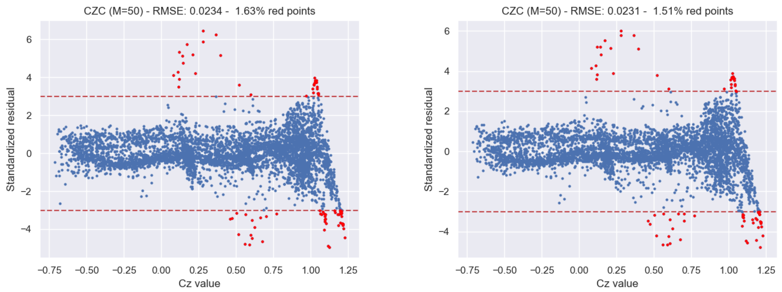
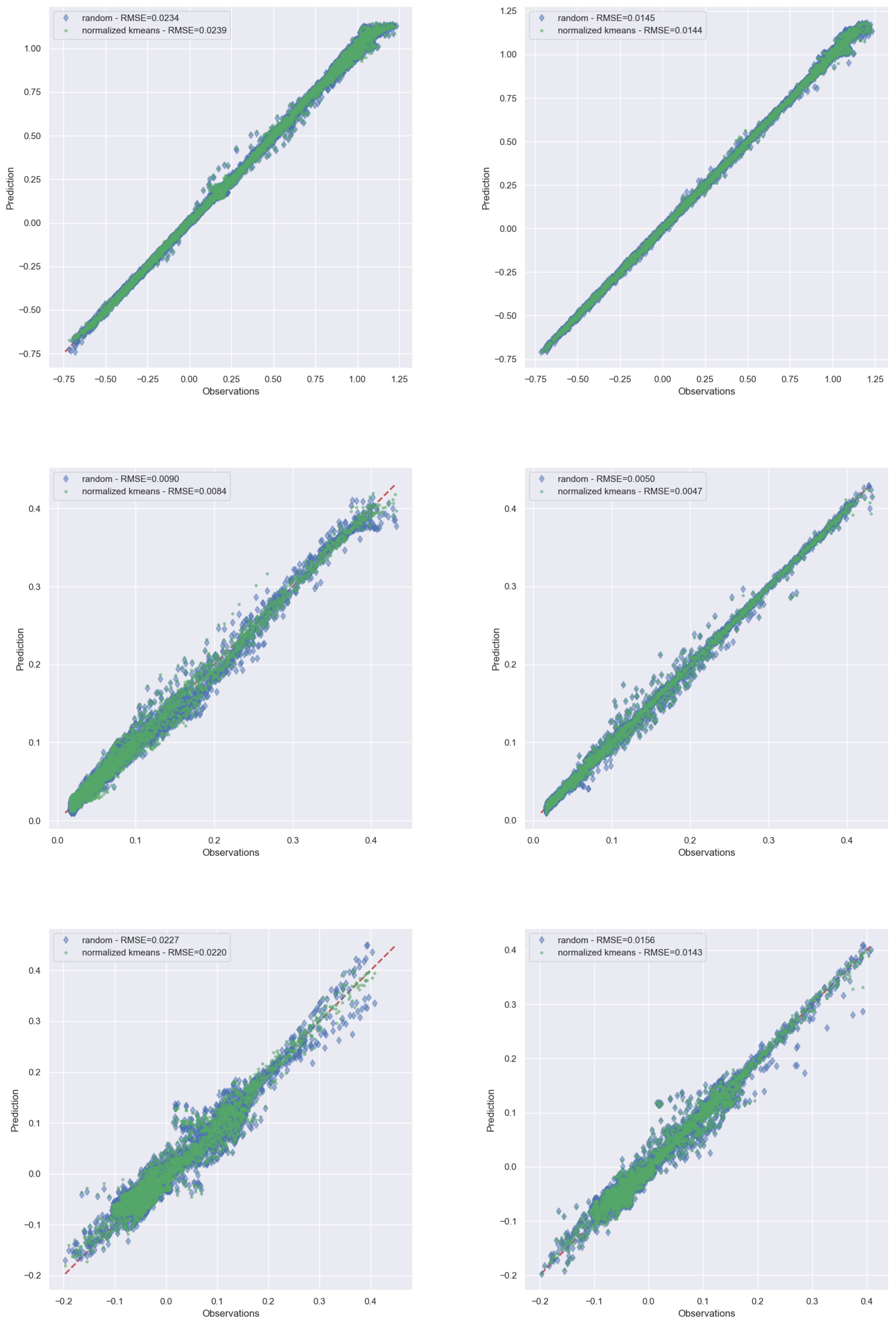
5.2. Results Analysis

As in [7], we consider an independent process, i.e., an SGP, for each outcome coefficient C x , C z , and C M , with a squared exponential kernel and with the default SMT parameters. Figure 9 presents a qualitative comparison between SGP-FITC and SGP-VFE predictions (50 random inducing points are used), where standardized residuals for the C z test set (5223 points) are computed from [34]:
Standardized residual ( x i ) = y ( x i ) y ^ ( x i ) s ( x i ) ,
where y ( x i ) corresponds to the observed value at point x i , y ^ ( x i ) for the GP prediction, and s ( x i ) for the estimated GP standard deviation. Standardized residuals are commonly used to identify potential outliers in regression analysis. Assuming that the data are normally distributed, then 99% of predictions should fall within ±3 s around the predictive GP mean. Due to the rescaling by s, then approximately 99 % of the standardized residuals should fall in the interval [ 3 , 3 ] . The region where the main deviation is observed corresponds to C z values close to 1, a value that typically corresponds to the wing stall region, and is highly sensitive to changes in the input variables. Despite the increased deviation compared to lower C z values, it remains within the interval [ 3 , 3 ] . Therefore, aside from a small number of predicted points (the red points), most of the residuals are within the confidence interval, suggesting an accurate fit of the regression model.
Table 3 summarizes the outcomes of a systematic study comparing the accuracy (i.e., the likelihood and RMSE) and computation time of both SGP-FITC and SGP-VFE across different values of M (ranging from 50 to 1000) for the three selection strategies of the inducing inputs. Similar to Section 4, the RMSE was computed on the training and test sets for a C z output. According to the results, the RMSE on the test data decreased as M increased, particularly between M = 100 and M = 500 . However, beyond this range, adding more inducing points did not yield meaningful RMSE improvements, and there was no significant impact between the random and the k-means-n schemes. The higher RMSE values led by the k-means are justified by the poor distribution of the inducing points. Generally speaking, both GP-FITC and GP-VFE show similar RMSE results. In Figure 10, the performance of the VFE and FITC methodologies is examined across various inducing point quantities: M = 50, 100, 500, and 1000. The primary focus lies in comparing the RMSE for each methodology. It is observed that in most inducing point scenarios, the k-means-n using the VFE emerges as the lower RMSE in general terms.
The CPU time involved by the k-means-based schemes, denoted in Table 3 as inducing time, is another criterion to analyze, as this step can be time-consuming. Therefore, it needs to be considered in addition to the training time. For the random selection, this inducing time is negligible, since it only involves a random permutation of the point indices. From Table 3, as expected, the inducing time of the k-means-based schemes increases as M increases. In particular, for the k-means scheme, the inducing time is more sensitive to M. For instance, for M = 1000 , the inducing time for k-means is almost three times higher than that of the k-means-n time. This substantial increase is due to the heterogeneity in the order of magnitude among the aerodynamic input parameters, making the convergence of the optimization relative to the clustering step slower. Thus, the normalization of both inputs and outputs in k-means-n proves beneficial in streamlining this process, consequently leading to a reduction in the computational overhead. Furthermore, it is noteworthy that both SGP-FITC and SGP-VFE demonstrate similar performance concerning the inducing time.
Complementary results on the quality of predictions for the outputs C z , C x , and C M are shown in Appendix A.2.2.

5.3. Results on a Testing Subset

To assess the impact of the inducing points distribution on the SGP predictability, the test database is now restricted to the region of the input domain not covered by the k-means scheme. To that aim, 1068 points satisfying the conditions α < 7 or α > 13 are retained. The distribution of training points and the new test subset points over the entire design space are depicted in Figure 11.
Figure 12 provides a visual representation of the cumulative density function (CDF) and boxplots of the squared prediction errors for the SGP-FITC with M = 50 . The figure compares the errors across three different selection schemes, providing a comprehensive understanding of the model’s performance under varying conditions. The squared prediction errors are computed for both the full test set (5223 points) and a subset of the test data (1286 points). The CDF curves illustrate the probability that a squared prediction error takes on a value less than or equal to x, providing insights into the distribution of these errors. By comparing the CDF curves of the three selection schemes, one can determine which scheme results in lower prediction errors. A curve that is shifted more towards the left indicates better performance, as it means that there is a higher probability of achieving lower prediction errors. Here, the k-means strategy is less efficient for reaching 1 (or 100% on the y-axis) with a maximum squared prediction error greater than 0.05 in both cases. The boxplots, on the other hand, offer a summary of the statistical features of these errors, including their median and quartiles. With some groups of three median lines relatively close, the whiskers of the box plot for k-means extend further than those for random and k-means-n schemes, indicating a larger range of error values and the presence of more extreme values. This figure serves as a valuable tool for assessing the performance of the SGP-FITC model and the impact of different selection schemes on its accuracy. As expected, the k-means performance is less consistent compared to the random and k-means-n schemes.

6. Discussion

For the WT database in Section 5, several conclusions can be drawn. First, the choice of the sparse approximation method (either the FITC or VFE) shows no significant impact on the analyzed criteria, whether in terms of global accuracy (i.e., the likelihood and RMSE) or in terms of the CPU times (i.e., inducing, training, and prediction times). Second, k-means performs poorly compared to the other methods (random and k-means-n), involving longer inducing times (due to the high differences in the order of magnitude between the inputs) and higher RMSE values (attributed to the poor distribution of inducing inputs in the design domain). Third, the random scheme shows similar RMSE values compared to k-means-n, with the advantage of requiring a negligible inducing time. However, the potential lack of robustness in the distribution of the inducing inputs may lead to a greater dispersion of performance and a possible reduction in the accuracy of the prediction, as observed in the analytical example studied in Section 4 and Appendix A.2.1. Therefore, the k-means-n scheme appears as a safer approach, more precisely when the number of inducing points is relatively low. Despite its non-negligible inducing time, k-means-n leads to accuracy improvements in terms of the likelihood and RMSE, as shown in Table 3.

7. Conclusions

To address the challenge of handling large datasets, we have explored SGP models, focusing on adapting two classic inference methods, namely the FITC and the VFE. Our study includes a comparative analysis of various strategies for selecting inducing inputs based on random or k-means methods, with or without normalization. Moreover, we have integrated our implementations into the open-source Python toolbox SMT. The versatility offered by this integration enhances the accessibility and applicability of SGP techniques in various applications. Lastly, the practical utility of our SGP developments is demonstrated through an analytical example and a real wind tunnel application featuring thousands of training data points. The performance showcased in these scenarios validates the approach.
The characterization and prediction of aircraft aerodynamics benefit from a collaborative approach involving both aerodynamic simulations and experiments. This tandem approach generates complementary datasets in terms of fidelity and cost, typically consisting of extensive data points. Multi-fidelity GPs are often used for mixing CFD simulations and wind tunnel experiments [7,12,35,36,37], but they cannot be applied to large databases. Hence, from a theoretical point of view, a potential future work is to extend the sparse approximations discussed in this paper to multi-fidelity GPs.
The next step for the developments involves integrating SGPs with other existing features in SMT. In particular, we aim to couple SGPs with the multi-fidelity and Bayesian optimization pipelines. This will enhance the capabilities of the toolbox by providing users with more advanced and versatile tools for surrogate modeling and optimization.

Author Contributions

Conceptualization, N.B., T.L., A.F.L.-L. and S.M; methodology, N.B., T.L., A.F.L.-L. and H.V.; software, R.L and H.V.; validation, N.B., M.C.-A., T.L., A.F.L.-L. and H.V.; formal analysis, A.F.L.-L. and H.V.; investigation, H.V.; data curation, R.L. and S.M.; writing—original draft preparation, N.B, R.L., A.F.L.-L. and H.V.; writing—review and editing, M.C.-A., T.L, A.F.L.-L. and S.M.; visualization, N.B., M.C.-A. and H.V.; supervision, N.B., T.L. and A.F.L.-L.; project administration, N.B. and S.M.; funding acquisition, N.B, A.F.L.-L. and S.M. All authors have read and agreed to the published version of the manuscript.

Funding

This work was supported by the ONERA internal research project dedicated to Hybridization, Optimization and Reliability methods for Uncertainty quantification in aerospace Systems, namely HORUS, and research visits at ONERA have been funded by the National Institute for Mathematical Sciences and Interactions (INSMI), CNRS, as part of the PEPS JCJC 2023 call.

Data Availability Statement

The numerical illustrations in Section 4 are publicly available in the Github repository: https://github.com/SMTorg/smt-sgp-paper (accessed on 26 March 2024).

Acknowledgments

The authors thank the role of the WT teams in the Modane-Avrieux and Le Fauga-Mauzac test centers (France) in creating the WT database, and especially Aurélia Cartieri.

Conflicts of Interest

The authors declare no conflicts of interest. The funders had no role in the design of the study; in the collection, analyses, or interpretation of the data; in the writing of the manuscript; or in the decision to publish the results.

Abbreviations

The following abbreviations are used in this manuscript:
HPCHigh-Performance Computing
GPGaussian Process
SGPSparse Gaussian Process
NMLLNegative Marginal Log-Likelihood
FITCFully Independent Training Conditional
VFEVariational Free Energy
KLKullback–Leibler
ELBOEvidence Lower Bound
SMTSurrogate Modeling Toolbox
DoEDesign of Experiments
RMSERoot Mean Square Error
WTWind Tunnel
CRMCommon Reference Model
CFDComputational Fluid Dynamics

Appendix A

Appendix A.1. Implementations of the FITC and VFE Methods in SMT

Since the expressions of both NMLL and NMLL V F E are similar, we will develop here the details of the implementation for the following general formulation:
NMLL = N 2 log ( 2 π ) + 1 2 log ( | K | ) + 1 2 y K 1 y + 1 2 η 2 tr ( T ) ,
where K can refer to either K F I T C or K V F E , and T F I T C = 0 while T V F E = K N N Q N N . We start by considering the Cholesky decomposition Q N N = V V . Hence, by introducing the one for the reduced covariance matrix K M M = U U , the Nyström approximation becomes:
V V = K M N U U 1 K M N = U 1 K M N U 1 K M N .
Therefore, we have V = U 1 K M N . Given this matrix, we can efficiently compute the other terms from the NMLL as follows:
  • The log-determinant term can be rewritten as:
    log ( | K | ) = log ( | V V + D + η 2 I N | ) = log ( | V V + D ˜ | ) ,
    where D is a diagonal matrix whithatch refers to either D F I T C = diag K N N Q N N or D V F E = 0 . Applying the matrix determinant lemma, we then have:
    V V + D ˜ = D ˜ . I N + V D ˜ 1 V = D ˜ . A .
    Hence, using the Cholesky decomposition A = L L , it can be shown that the log-determinant term can also be expressed as:
    log ( | K | ) = i d i + 2 i L i i ,
    where d i is the vector containing the diagonal terms of D ˜ , whose computations are straightforward but slightly different between the FITC and VFE methods given their respective definitions.
  • The quadratic term, also referred to as the “Mahalanobis” term, is computed using the Woodbury matrix identity to obtain the inverse of K :
    K 1 = V V + D ˜ 1 = D ˜ 1 D ˜ 1 V A 1 V D ˜ 1 .
    Thus, as D ˜ is a diagonal matrix, we can simply replace it with the inverse of the vector d computed beforehand. By relying again on the factorization of matrix A , we can still gain in efficiency by noticing the following:
    K 1 = d 1 + d 1 V L L 1 V d 1 = d 1 + L 1 V d 1 L 1 V d 1 .
    Hence, the computation is straightforward, as we only need to compute the inverse of vector d and of triangular factor L .
  • The trace term (only appearing in the VFE method) does not present any particular difficulty; relying on the Cholesky decomposition of Q N N , we obtain the following:
    tr K N N Q N N = tr K N N tr V V .
Therefore, the computations involved here allow us to maintain reasonable scalability, since we limit the complexity to M × M triangular matrice inversions, avoid most of the required matrix products, and keep a memory cost up to the storage of an M × N matrix.

Appendix A.2. Complementary Results

Appendix A.2.1. Analytic Example

Figure A1 illustrates another sampling where the random selection of inducing points ( M = 30 ) can give poor predictions when some area is not sufficiently covered (here x [ 1 , 0.75 ] ) compared to the k-means choice.
Figure A1. Prediction obtained by SGP-FITC with M = 30 inducing points chosen via random (top) and k-means (bottom) schemes. Each panel shows the target function (orange solid line), the training data (blue points), the predictive mean (black solid line), and the 99% confidence intervals (dashed green lines) led by the models. For the SGPs, the M = 30 inducing inputs are shown along the x-axis.
Aerospace 11 00260 g0a1

Appendix A.2.2. WT Application

Figure A2 shows the prediction Q–Q plots of the SGP-FITC for the outputs C z , C x , and C M , and considering random and k-means-n schemes with M = 50 , 500 .
Figure A2. Q–Q plots for the outputs C z (top), C x (center), and C M (bottom) using a GP-FITC with M = 50 (left) or 500 (right). The results are shown for the random (blue points) and k-means-n (green points) schemes for the selection of the inducing points.
Aerospace 11 00260 g0a2

References

  1. Svendsen, D.H.; Martino, L.; Camps-Valls, G. Active Emulation of Computer Codes with Gaussian Processes— Application to Remote Sensing. Pattern Recognit. 2020, 100, 107103. [Google Scholar] [CrossRef]
  2. Slotnick, J.; Khodadoust, A.; Alonso, J.; Darmofal, D.; Gropp, W.; Lurie, E.; Mavripilis, D. CFD Vision 2030 Study: A Path to Revolutionary Computational Aerosciences. In NASA Technical Report; NASA/CR-2014-218178; NASA: Washington, DC, USA, 2014; pp. 1–51. [Google Scholar]
  3. Malik, M.; Bushnell, D. Role of Computational Fluid Dynamics andWind Tunnels in Aeronautics R and D. In NASA Technical Report; NASA/TP–2012-217602; NASA: Washington, DC, USA, 2012; pp. 1–63. [Google Scholar]
  4. Yondo, R.; Bobrowski, K.; Andres, E.; Valero, E. A Review of Surrogate Modeling Techniques for Aerodynamic Analysis and Optimization: Current Limitations and Future Challenges in Industry. In Advances in Evolutionary and Deterministic Methods for Design, Optimization and Control in Engineering and Sciences; Springer International Publishing: Berlin/Heidelberg, Germany, 2019; pp. 19–33. [Google Scholar]
  5. Andrés-Pérez, E.; Paulete-Periáñez, C. On the Application of Surrogate Regression Models for Aerodynamic Coefficient Prediction. Complex Intell. Syst. 2021, 7, 1991–2021. [Google Scholar] [CrossRef]
  6. Giangaspero, G.; MacManus, D.; Goulos, I. Surrogate Models for the Prediction of the Aerodynamic Performance of Exhaust Systems. Aerosp. Sci. Technol. 2019, 92, 77–90. [Google Scholar] [CrossRef]
  7. Arenzana, R.C.; López-lopera, A.F.; Mouton, S.; Bartoli, N.; Lefebvre, T. Multi-Fidelity Gaussian Process Model for CFD and Wind Tunnel Data Fusion. In Proceedings of the Aerobest (An ECCOMAS Conference on Multidisciplinary Design Optimization of Aerospace Systems), Lisbon, Portugal (online conference), 21–23 July 2021; pp. 98–119. [Google Scholar]
  8. López-Lopera, A.F.; Idier, D.; Rohmer, J.; Bachoc, F. Multioutput Gaussian Processes with Functional Data: A Study on Coastal Flood Hazard Assessment. Reliab. Eng. Syst. Saf. 2022, 218, 108139. [Google Scholar] [CrossRef]
  9. Forrester, A.; Sobester, A.; Keane, A. Multi-Fidelity Optimization via Surrogate Modelling. Proc. R. Soc. A 2007, 463, 3251–3269. [Google Scholar] [CrossRef]
  10. Fu, W.; Chen, Z.; Luo, J. Aerodynamic Uncertainty Quantification of a Low-Pressure Turbine Cascade by an Adaptive Gaussian Process. Aerospace 2023, 10, 1022. [Google Scholar] [CrossRef]
  11. Pham, V.; Tyan, M.; Nguyen, T.A.; Lee, J.W. Extended Hierarchical Kriging Method for Aerodynamic Model Generation Incorporating Multiple Low-Fidelity Datasets. Aerospace 2024, 11, 6. [Google Scholar] [CrossRef]
  12. Meliani, M.; Bartoli, N.; Lefebvre, T.; Bouhlel, M.; Martins, J.; Morlier, J. Multi-Fidelity Efficient Global Optimization: Methodology and Application to Airfoil Shape Design. In Proceedings of the AIAA Aviation Forum, Dallas, TX, USA, 17–21 June 2019; pp. 1–18. [Google Scholar]
  13. Rasmussen, C.; Williams, C. Gaussian Processes for Machine Learning (Adaptive Computation and Machine Learning); The MIT Press: Cambridge, MA, USA, 2005. [Google Scholar]
  14. Quiñonero Candela, J.; Rasmussen, C. A Unifying View of Sparse Approximate Gaussian Process Regression. J. Mach. Learn. Res. 2005, 6, 1939–1959. [Google Scholar]
  15. Snelson, E.; Ghahramani, Z. Sparse Gaussian Processes using Pseudo-inputs. Adv. Neural Inf. Process. Syst. 2005, 18, 1257–1264. [Google Scholar]
  16. Titsias, M.K. Variational Learning of Inducing Variables in Sparse Gaussian Processes. J. Mach. Learn. Res. Proc. Track 2009, 5, 567–574. [Google Scholar]
  17. Van Der Wilk, M. Sparse Gaussian Process Approximations and Applications. Ph.D. Thesis, University of Cambridge, Cambridge, UK, 2019. [Google Scholar]
  18. Liu, H.; Ong, Y.S.; Shen, X.; Cai, J. When Gaussian Process Meets Big Data: A Review of Scalable GPs. IEEE Trans. Neural Netw. Learn. Syst. 2020, 31, 4405–4423. [Google Scholar] [CrossRef] [PubMed]
  19. Bouhlel, M.A.; Hwang, J.T.; Bartoli, N.; Lafage, R.; Morlier, J.; Martins, J.R. A Python Surrogate Modeling Framework with Derivatives. Adv. Eng. Softw. 2019, 135, 102662. [Google Scholar] [CrossRef]
  20. Titsias, M.K. Variational Model Selection for Sparse Gaussian Process Regression; Technical report; University of Manchester, School of Computer Science: Manchester, UK, 2009. [Google Scholar]
  21. Bauer, M.; van der Wilk, M.; Rasmussen, C.E. Understanding Probabilistic Sparse Gaussian Process Approximations. In Advances in Neural Information Processing Systems; Lee, D., Sugiyama, M., Luxburg, U., Guyon, I., Garnett, R., Eds.; Curran Associates, Inc.: Red Hook, New York, USA, 2016; Volume 29. [Google Scholar]
  22. Saves, P.; Lafage, R.; Bartoli, N.; Diouane, Y.; Bussemaker, J.; Lefebvre, T.; Hwang, J.T.; Morlier, J.; Martins, J.R. SMT 2.0: A Surrogate Modeling Toolbox with a Focus on Hierarchical and Mixed Variables Gaussian Processes. Adv. Eng. Softw. 2024, 188, 103571. [Google Scholar] [CrossRef]
  23. GPy: A Gaussian Process Framework in Python. 2012. Available online: https://gpy.readthedocs.io/en/deploy/ (accessed on 10 January 2024).
  24. Matthews, A.G.d.G.; van der Wilk, M.; Nickson, T.; Fujii, K.; Boukouvalas, A.; León-Villagrá, P.; Ghahramani, Z.; Hensman, J. GPflow: A Gaussian Process Library using TensorFlow. J. Mach. Learn. Res. 2017, 18, 1–6. [Google Scholar]
  25. Hensman, J.; Fusi, N.; Lawrence, N.D. Gaussian Processes for Big Data. In Proceedings of the Twenty-Ninth Conference on Uncertainty in Artificial Intelligence, Arlington, VA, USA, 11–15 July 2013; pp. 282–290. [Google Scholar]
  26. Ester, M.; Kriegel, H.P.; Sander, J.; Xu, X. A density-based algorithm for discovering clusters in large spatial databases with noise. In Proceedings of the 2nd International Conference on Knowledge Discovery and Data Mining, Portland, OR, USA, 2–4 August 1996; AAAI Press: Washington, DC, USA, 1996. KDD’96. pp. 226–231. [Google Scholar]
  27. Vassberg, J.; Dehaan, M.; Rivers, M.; Wahls, R. Development of a Common Research Model for Applied CFD Validation Studies. In Proceedings of the 26th AIAA Applied Aerodynamics Conference, Honolulu, HI, USA, 18–21 August 2008; American Institute of Aeronautics and Astronautics: Reston, VA, USA, 2008; pp. 1–22. [Google Scholar]
  28. Carrara, J.; Masson, A. Three Years of Operation of the ONERA Pressurized Subsonic Wind Tunnel. In Proceedings of the 12th Congress of the International Council of the Aeronautical Sciences, Munich, Germany, 12–17 October 1980; pp. 778–792. [Google Scholar]
  29. Cartieri, A.; Hue, D.; Chanzy, A.; Atinault, O. Experimental Investigations on Common Research Model at ONERA-S1MA–Drag Prediction Workshop Numerical Results. J. Aircr. 2017, 55, 1491–1508. [Google Scholar] [CrossRef]
  30. Rivers, M.; Dittberner, A. Experimental Investigation of the NASA Common Research Model. In Proceedings of the 28th AIAA Applied Aerodynamics Conference, Chicago, IL, USA, 28 June–1 July 2010; pp. 1–29. [Google Scholar]
  31. Rivers, M.; Quest, J.; Rudnik, R. Comparison of the NASA Common Research Model European Transonic Wind Tunnel Test Data to NASA National Transonic Facility Test Data. Ceas Aeronaut. J. 2018, 9, 307–317. [Google Scholar] [CrossRef]
  32. Hantrais-Gervois, J.; Piat, J. A Methodology to Derive Wind Tunnel Wall Corrections from RANS Simulations. In Proceedings of the Advanced Wind Tunnel Boundary Simulation, ST0/NATO, Torino, Italy, 16–18 April 2018; pp. 1–24. [Google Scholar]
  33. Cartieri, A.; Hue, D. Using RANS Computations to Calculate Support Interference Effects on the Common Research Model. In Proceedings of the Advanced Wind Tunnel Boundary Simulation, ST0/NATO, Torino, Italy, 16–18 April 2018; pp. 1–18. [Google Scholar]
  34. Jones, D.R.; Schonlau, M.; Welch, W.J. Efficient Global Optimization of Expensive Black-Box Functions. J. Glob. Optim. 1998, 13, 455–492. [Google Scholar] [CrossRef]
  35. Bertram, A.; Zimmermann, R. Theoretical Investigations of the New CoKriging Method for Variable-Fidelity Surrogate Modeling: Well-Posedness and Maximum Likelihood Training. Adv. Comput. Math. 2018, 44, 1693–1716. [Google Scholar] [CrossRef]
  36. Stradtner, M.; Liersch, C.; Bekemeyer, P. An Aerodynamic Variable-Fidelity Modelling Framework for a Low-Observable UCAV. Aerosp. Sci. Technol. 2020, 107, 106232. [Google Scholar] [CrossRef]
  37. Bekemeyer, P.; Bertram, A.; Hines Chaves, D.A.; Dias Ribeiro, M.; Garbo, A.; Kiener, A.; Sabater, C.; Stradtner, M.; Wassing, S.; Widhalm, M.; et al. Data-driven aerodynamic modeling using the DLR SMARTy toolbox. In Proceedings of the AIAA Aviation 2022 Forum, Chicago, IL, USA, 27 June–1 July 2022; p. 3899. [Google Scholar]
Figure 1. SGP in the SMT 2.3 architecture.
Aerospace 11 00260 g001
Figure 2. 1D analytical example (orange solid line) with 200 noisy training data points (blue points). The M = 30 randomly selected inducing inputs are represented by red bars along the x-axis.
Aerospace 11 00260 g002
Figure 3. Predictions for the example in Figure 2 obtained by SGPs using both the FITC (top) and VFE (center), and by an exact GP (bottom). Each panel shows: the target function (orange solid line), the training data (blue points), the predictive mean (black solid line), and 99% confidence intervals (dashed green lines) led by the models. For the SGPs, the inducing inputs are shown along the x-axis.
Aerospace 11 00260 g003
Figure 4. Training time curves for the exact GP (red) and SGP-FITC (blue) inference as a function of the number of training points N. The theoretical and empirical profiles are shown in solid and dashed lines, respectively. For the SGP-FITC, M has been fixed to 10. To recall, inference for the SGP scales linearly as O ( N M ) , whereas that of the exact GP scales quadratically as O ( N 2 ) .
Aerospace 11 00260 g004
Figure 5. Location of the inducing points for the analytical example in Figure 2 considering the random (red bars) and k-means-based (black crosses) selection schemes.
Aerospace 11 00260 g005
Figure 6. Prediction obtained by SGP-FITC with M = 30 inducing points chosen via k-means. The panel description is as in Figure 3.
Aerospace 11 00260 g006
Figure 7. Histograms of the four input variables ( M a c h , R e , α , β ): training points (47,004 points in blue) and test points (5223 points in orange).
Aerospace 11 00260 g007
Figure 8. Distribution of the C z training points (47,004, blue points) and M = 50 inducing inputs considering three design schemes: random (top, red points), k-means (center, black points), and k-means-n (bottom, green points).
Aerospace 11 00260 g008
Figure 9. Standardized residual for the C z test set (5223 points) using SGP-FITC (left) or SGP-VFE (right). The residual points outside the [ 3 , 3 ] confidence intervals are displayed in red.
Aerospace 11 00260 g009
Figure 10. Comparison of RMSE for SGP-FITC and SGP-VFE methodologies across M = 50, 100, 500, and 1000 inducing points.
Aerospace 11 00260 g010
Figure 11. Histograms of the four input variables ( M a c h , R e , α , β ): training points (47,004 points in blue) and test points (1286 points in orange).
Aerospace 11 00260 g011
Figure 12. Output C z : cumulative density function and boxplot for the squared prediction errors using the full test set of 5223 points (left column) or the subset of 1286 points (right columns). GP-FITC is used with M = 50 inducing points chosen randomly, with k-means or k-means-n (normalized k-means).
Aerospace 11 00260 g012
Table 1. Comparison of the optimal GP parameters, training time, likelihood, and RMSE for the GP-based models in Figure 3.
SGP-FITCSGP-VFEExact GP
Optimal σ 2 4.780.810.88
Optimal θ 37.0444.8020.96
Optimal η 2 (noise)0.0100.0120.011
Training time [s]0.190.180.42
Optimal likelihood280.11266.99303.90
RMSE-training data0.09620.09690.0945
RMSE-test data0.11050.10920.1050
Table 2. Comparison of the optimal GP parameters, training time, likelihood, and RMSE for the SGP-based models using the k-means configuration of inducing points from Figure 6 ( M = 30 ).
SGP-FITCSGP-VFEExact GP
Optimal σ 2 0.700.800.88
Optimal θ 56.8454.4220.96
Optimal η 2 (noise)0.0100.0130.011
Training time [s]0.190.180.42
Optimal likelihood282.99276.63303.90
RMSE-training data0.09660.09640.0945
RMSE-test data0.11530.11150.1050
Table 3. Output C z : comparison of the likelihood, RMSE, and CPU times on the training and test datasets with M = 50 , 100 , 500 , 1000 , considering different schemes for the selection of the inducing points. The strategy of applying k-means with normalized data is denoted as k-means-n. The CPU time involved by the selection of the inducing inputs is denoted as inducing time. The arrows show whether the metric has risen (🡹) or fallen (🡻) in comparison to the results achieved with M = 50 . The colors signify the nature of the behavior, with green indicating positive or favorable trends, and red indicating negative or unfavorable trends. For each SGP model, the best results across the different selection schemes are highlighted in bold.
SGP-FITCSGP-VFE
Randomk-Meansk-Means-nRandomk-Meansk-Means-n
M = 50
Likelihood150,709147,636150,614147,646137,891147,919
RMSE-training data0.02570.02620.02460.02480.03140.0251
RMSE-test data0.02670.02670.02490.02470.03140.0248
Inducing time≈0510≈079
Training time191920191919
Prediction time0.020.010.020.020.020.02
M = 100
Likelihood (🡹)161,201155,554157,966156,422148,673158,380
RMSE-training data (🡻)0.02050.02270.02090.02050.02400.0202
RMSE-test data (🡻)0.02060.02220.02120.02030.02370.0201
Inducing time (🡹)≈02418≈03319
Training time (🡹)404042564038
Prediction time (🡹)0.030.040.040.040.040.04
M = 500
Likelihood (🡹)172,894171,246173,187171,502161,872172,228
RMSE-training data (🡻)0.01450.01790.01480.01470.01770.0145
RMSE-test data (🡻)0.01500.01750.01480.01510.01740.0148
Inducing time (🡹)≈033390≈032689
Training time (🡹)218219219213213213
Prediction time (🡹)0.170.170.170.170.170.17
M = 1000
Likelihood (🡹)172,704173,003175,620172,884165,026175,077
RMSE-training data (🡻)0.01440.01570.01340.01430.01650.0136
RMSE-test data (🡻)0.01470.01550.01380.01470.01620.0140
Inducing time (🡹)≈0319127≈0296125
Training time (🡹)471472475464471461
Prediction time (🡹)0.340.340.340.340.360.34
Disclaimer/Publisher’s Note: The statements, opinions and data contained in all publications are solely those of the individual author(s) and contributor(s) and not of MDPI and/or the editor(s). MDPI and/or the editor(s) disclaim responsibility for any injury to people or property resulting from any ideas, methods, instructions or products referred to in the content.

