1. Introduction
Reynolds Averaged Navier–Stokes Equation (RANS) equations, in combination with eddy viscosity turbulence models based on the Boussinesq assumption, build the foundation of computational fluid dynamics simulations in aircraft development. On the one hand, these simulations can predict aerodynamic behavior at satisfactory accuracy levels for most investigated configurations while providing comparatively low costs and robustness. On the other hand, the models lack accuracy at higher angles of attack for leading-edge vortex flow systems of mid to low aspect-ratio delta wing configurations since they cannot represent the effects on streamline curvature and system rotation. Shur et al., introduced a streamline curvature correction (SARC) approach by multiplying the production term in the original Spalart–Allmaras (SA) turbulence model by a rotation function [
1]. Further, this modification has been implemented to the Shear Stress Transport (SST) turbulence model of Menter [
2,
3]. Two approaches to account for the effects of rotation and curvature are explored by Arolla et al. [
4]. The “Modified coefficients approach” aims to alter the growth rate of the turbulent kinetic energy, whereas the “Bifurcation approach” adjusts the eddy viscosity coefficient such that the equilibrium solution bifurcates from healthy to decaying solutions. While most of the available turbulence model corrections for this type of flow aim at maintaining the globality of the fundamental turbulence model, Moioli et al., developed an adaptive turbulence model based on the one-equation SA turbulence model [
5,
6]. Moioli et al., introduced additional source terms controlled by model coefficients and a switch factor (i–vii in Equation (1)), which is only effective in vortex-dominated flow regions and switches off the added source terms in unaffected regions of the flow.
The model coefficients can be set via a gradient descent approach optimization procedure based on experimental or high-fidelity simulation data. Further, in the field of turbulence modeling, Duraisamy et al., pointed out the expanding importance of data-driven models and techniques in computational fluid dynamics (CFD) [
7]. The increase in computational power, e.g., on the side of graphical processing units, leads to the development of new machine learning algorithms and enables the usage of existing ones, taking advantage of the vast amount of available data from experimental and numerical studies. Deep learning architectures have been shown to represent high-level abstractions in various fields [
8]. Sabater et al., develop three fast prediction tools to predict aircraft surface pressure distribution using different machine learning techniques [
9]. Their study shows that deep-learning methods outperform others by accurately predicting shock wave locations and strength in transonic flows. The characteristics of transonic buffet are predicted by a reduced-order modeling (ROM) framework based on a long short-term memory (LSTM) neural network in the work of Zahn et al. [
10]. Zhang et al., used convolutional neural network (CNN) architectures to predict lift coefficient based on airfoil shape and flow conditions.
The objective of this work is to develop a data-driven methodology for the preconditioning of the enhanced SA turbulence model (Equation (1)) by Moioli et al., and highlight the benefits of a low-cost preconditioning framework [
5]. While the enhanced model is specially tailored for leading-edge vortex flows of mid to low aspect-ratio delta wings, the framework shall be independent of the aircraft configuration. The predictive capabilities are discussed for a generic triple delta wing test case in
Section 7.
2. Test Cases: Generic Multiple Swept Delta Wings
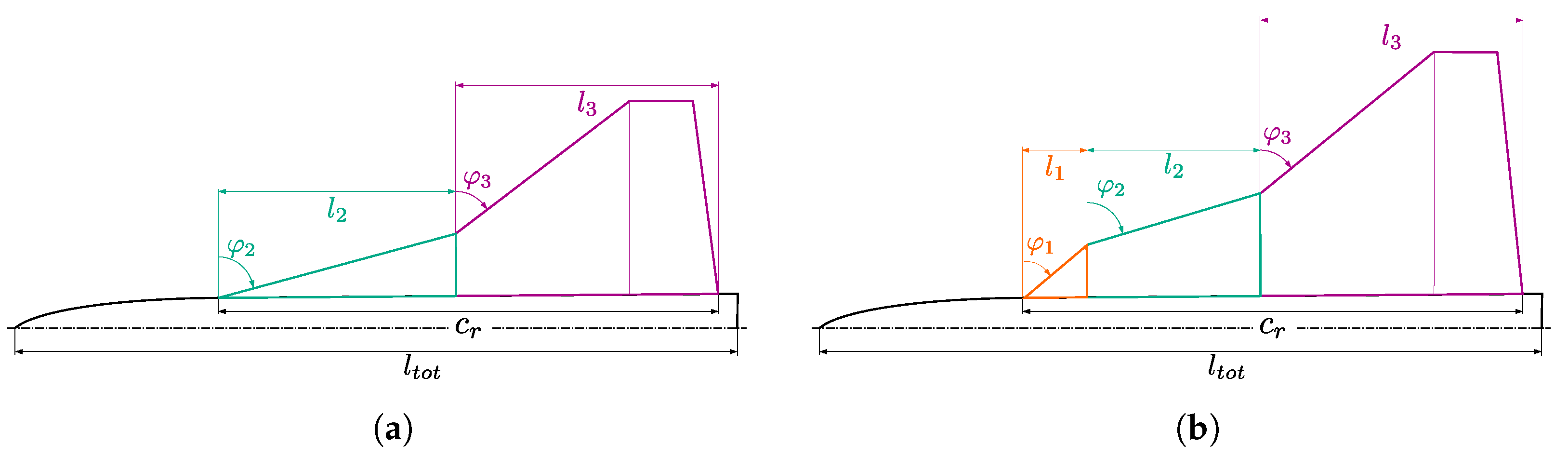
This study considers generic wing-fuselage configurations in the form of triple and double delta wing configurations with varying leading-edge sweep angles. The wind tunnel models consist of a fuselage and interchangeable flat plate wings with sharp leading-edges. Each configuration type is also equipped with deflectable control surfaces, e.g., levcons for triple delta wings and slats for double and triple delta wings.
These geometries were and are subject to a common research program in cooperation with Airbus Defence and Space and the German Aerospace Center and are further embedded in the NATO AVT-316 task group [
11]. Various experimental and numerical studies have been performed for a range of configurations [
12,
13,
14,
15].
Table 1 lists the most important geometrical parameters of the two configuration types. An overview of the two different types is also depicted in
Figure 1a,b. For this study, five triple and five double delta wing plan forms serve as training datasets for the machine learning framework. Further, the designation of different configurations follows the initial convention developed by Airbus Defence and Space. E.g., the platform F3 607060 STLong LV00 SL00 FL00 describes a triple delta wing (F3) with a
levcon sweep angle
, a
strake sweep angle
, and a main wing sweep angle of
. STLong designates the long strake section of the two possible values for
in
Table 1, whereas STShort would designate the shorter version. The abbreviations LV, SL, and FL, followed by the number 00, describe the zero deflection angles for the different available control surfaces levcon (LV), slat (SL), and flap (FL).
3. Numerical Setup
The TAU-Code (triangular adaptive upwind) developed by DLR is used as the fundamental flow solver. The DLR TAU-Code is widely accepted in the aviation industry and provides a tool to run complex flow simulations on structured and unstructured hybrid grids. It represents not one simple code but a modern software system to compute inviscid and viscous flows at various flow velocities for simple and complex geometries. The TAU system is composed of different modules and libraries to allow for the easier development, maintenance, and reuse of the code or parts of it. Single modules can be used as stand-alone tools with a specific file I/O or in combination with a Python scripting framework, allowing inter-module communication and enabling interaction with a started simulation [
16]. The flow calculations are based on the dual grid approach, which gives good results for three-dimensional hybrid grids. The Runge–Kutta dual time stepping method or a backward Euler implicit scheme are used as a time-marching method to solve three-dimensional Navier–Stokes equations with LU-SGS (lower-upper symmetric Gauss-Seidel) or SGS iterations. The optimization process described in
Section 5 is coupled with TAU via a Python framework (Python 3.8.16).
All simulations have been performed at a Mach number
and a Reynolds number
to resemble the experiments conducted in the wind tunnel of the Chair of Aerodynamics and Fluid Mechanics at the Technical University of Munich by Pfnür et al. [
12]. The CENTAUR meshing software has been used to create numerical grids as hybrid unstructured grids with prism layers and tetraeders. A grid study has been performed for the generic double delta wing with a strake sweep angle of
and a main wing sweep angle of
.
Figure 2 presents the results of the conducted gridstudy. For each of the five different grid resolutions, a simulation at the angle of attack
has been performed. The lift coefficient results in the left part of
Figure 2 show that all grid resolutions represent the experimentally obtained lift coefficient rather well. The results of the pitching moment coefficient in the right hand of
Figure 2 show that all grid resolutions deviate from the experimental value. The results show that there is no improvement in accuracy from the fine grid level to the very fine grid level.
Considering the results of the grid study and the high number of simulations needed to generate the training dataset, the medium grid resolution has been selected. This grid level has
elements, and the numerical grids of all different configurations have been kept as similar as possible.
Figure 3 shows a sample of the medium-sized double delta wing grid.
4. Adaptive Turbulence Model
The additional source terms of the adaptive turbulence model in Equation (1) are controlled via corresponding additional turbulence model coefficients and other flow quantities, limiting the added terms’ influence region to vortex-dominated flow regions only. Thus, the vortex identifier
is the most important control quantity. Based on the works of Truesdell and Jeong et al., Moioli et al., implemented the vortex identifier quantity based on the definition that a vortex can be defined as the region where the kinematic vorticity number
is greater than one [
17,
18]. From the definition
, the vortex identifier is defined as,
where
is a small number to avoid numerical overflow in the case the strain rate takes on values close to zero [
5]. The offset by the
coefficient is needed to remove the influence of terms multiplied by
in the boundary layer.
This work will focus on the terms
i,
v, and
in Equation (1), which will be introduced in detail in the following.
is the first added source term, which is only influenced by the vortex identifier and is the most similar one to the original SA source term
. Secondly, the coefficient
is multiplied by
and the normalized helicity
. The Helicity
expresses the alignment of velocity and vorticity vectors. The unburst part of a vortex shows high axial and rotational velocities, where the vorticity is increased along axial direction [
19]. Thus, the source term
acts in regions of fully developed healthy vortices. To prevent the turbulence model from acting differently for right and left-rotating vortices, it is important to use the absolute value of the helicity since the quantity also considers the vortex’s chirality. In order to non-dimensionalize all added quantities, the absolute value of helicity is normalized by the free-stream velocity, resulting in a final non-dimensional helicity
. The flow regions downstream of vortex breakdown are influenced by an inverted helicity-based term and the coefficient
. Caused by abrupt changes in rotational and axial velocities, vortex breakdown can be enclosed by regions of high-velocity gradients. Thus, the coefficient
, combined with the velocity gradient tensor and the vorticity direction, mainly influences regions near vortex breakdown.
Figure 4 shows the influence of three additional turbulence model coefficients for an exemplary double delta wing configuration.
5. Optimization of Additional Turbulence Model Coefficients
The coefficients of the additional source terms can be determined by an optimization scheme based on gradient descent optimization [
5]. The iterative algorithm minimizes the objective function
, which is defined as the L-1 norm between numerical and experimental data and is defined as:
where
k is the number of design points, e.g., angles of attack, and
l is the number of experimental coefficients, e.g., the lift coefficient
and pitching moment coefficient
. The importance of experimental reference values can be adjusted by weighting factors
.
itself is the deviation of numerical from experimental coefficients.
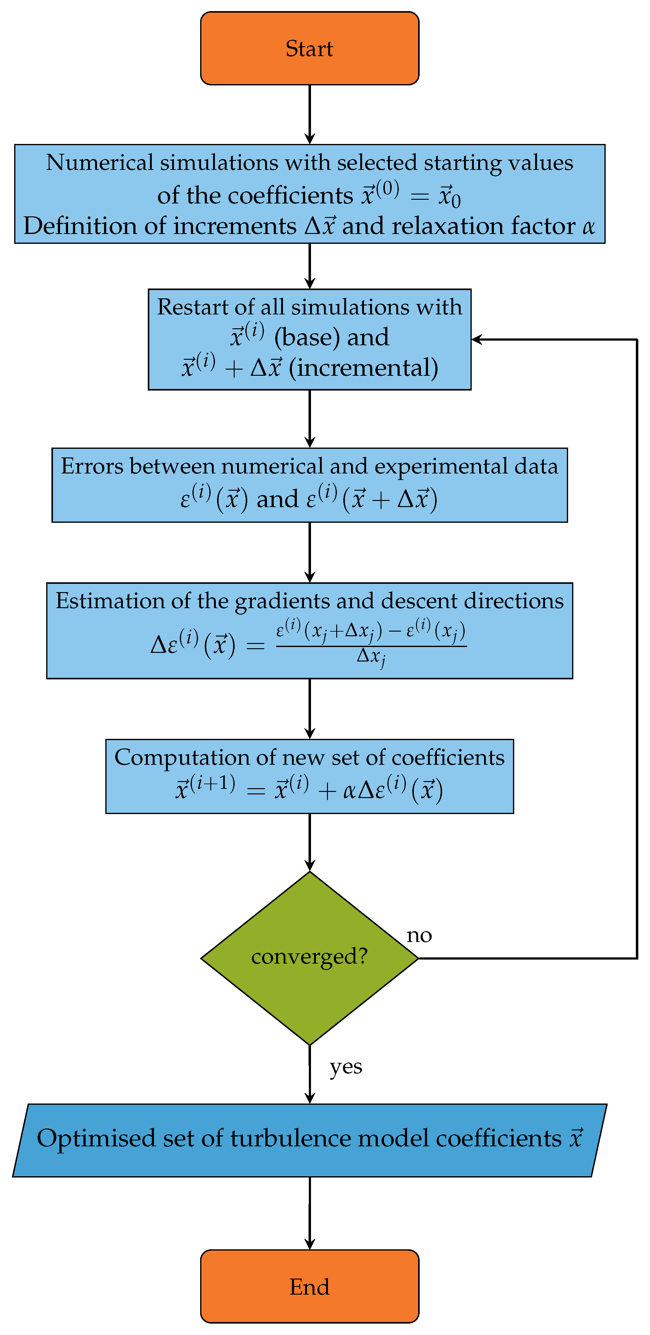
Figure 5 depicts the optimization process flowchart, where a case is started by selecting a set of starting values
.
Further, different increments
for each coefficient and an overall relaxation factor
need to be defined. Based on the initial settings, a series of numerical simulations is started, where a base simulation with the currently defined turbulence model coefficients is executed first. After this first base simulation is finished, the so-called incremental simulations are started, where for each included turbulence model coefficient a simulation is started after the predefined increment alters the base coefficient. A second base simulation continues the first base simulation to keep a consistent base solution throughout the process. Once the second base and all incremental simulations have finished, the errors concerning the linked experimental reference values can be computed. Experimental values can consist of aerodynamic coefficients, integral forces, surface pressure distributions from time-resolved pressure sensitive paint (iPSP) or pressure tabs. Due to the availability of aerodynamic coefficients for several configurations included in the generic wing-body platform described in
Section 2, this type of reference value has been chosen.
From the computed errors, the gradients and descent directions can be computed. Finally, a new updated set of turbulence model coefficients is defined by:
where
is the defined relaxation factor to avoid overshooting during the optimization procedure, which is set at
for this study. Once the new set of coefficients has been defined, it needs to be checked if the results have converged. If a satisfying level of convergence is reached, the optimization is ended with the set of turbulence model coefficients. If no convergence is reached, the optimization loop is restarted with the new set of coefficients serving as the new base. Since the gradient descent approach is inherently local and converges to local minima, cases with different starting points
should be run to increase the likelihood of finding a global optimum [
5].
Figure 6 depicts a sample of an optimization run. The objective function
is plotted versus the optimization iterations in the top part of the figure. The three additional turbulence values used are plotted against the corresponding iterations in the lower part.
6. Hybrid Neural Network
The ultimate goal of this study is to implement a machine learning framework that can predict the additional turbulence model coefficients based on a small number of inputs rather than rely on the optimization procedure described in
Section 5. Moioli et al., showed that an optimized set of turbulence model coefficients for one configuration case is not necessarily beneficial for a similar problem [
20]. Further, experimental reference values for the needed or selected design points are not always available. Thus, the optimization routine is not applicable if the enhanced turbulence model should be deployed in large-scale production or applied for many different cases, e.g., in an early aircraft design phase with new configuration types.
The basic idea is to design a machine learning framework to predict selected additional turbulence model coefficients. This data model outputs the proper set of coefficients based on the geometrical properties of the configuration under investigation, flow, or flight parameters. The proposed hybrid neural network (HNN) is depicted in
Figure 7. The neural network consists of a CNN segment, a fully connected layer with additional inputs, and an attached feed-forward neural network part.
A CNN is used for the geometry recognition and feature extraction to achieve maximum flexibility with respect to the input geometry. CNNs are known for their vast capabilities in image and pattern recognition, which enables the prediction framework to be independent of the input configuration. Rather than hard-coded input neurons for different geometric properties, a simple graphic of the wing-body plan form of the configuration is read in and propagated through several convolutional layers, including max-pooling and layer normalization. This architecture allows one network to be used for all thinkable cases since, e.g., a single delta wing configuration would have only one leading-edge sweep angle as a parameter, whereas in contrast, a triple delta wing configuration would have three distinct leading-edge sweep angles as input. Although high-aspect ratio wings are not part of the intended use cases, the implemented network could be fed with a plan form of the NASA Common Research Model (CRM). In the fully connected layer, the output of the CNN is combined with additional inputs. These inputs include the angle of attack and the Mach number , and since the graphics of the input plan forms are not in scale, the aspect ratio is added. Due to the relatively small training data set, each iteration of each case optimization serves as a data point. To differentiate between proper coefficients and unwanted sets of coefficients during training, the objective function as well as the errors between numerical and experimental aerodynamic coefficients and are added as inputs. The turbulence model coefficients are predicted in the final output layer after a series of hidden layers in a feed-forward neural network segment.
Hyperparameter Optimization and Training
The hyperparameter optimization is realized using the Optuna framework [
21]. As a define-by-run optimization framework, Optuna has been mainly developed for the hyperparameter optimization of neural networks. The efficient implementation and the versatile architecture, which enable an easy setup of the optimization runs, are critical elements of the software. The framework implements a Tree-structured Parzen Estimator (TPE) algorithm with an additional pruning mechanism. Pruning itself can be seen as an early-stopping method, where the algorithm detects automatically if the current trial shows promising results compared to a set of earlier trials or if the current trial should be canceled and another trial with a new set of hyperparameters should be started [
21].
Table 2 lists the most important hyperparameters of the HNN.
The available trainings dataset was obtained by conducting coefficient optimizations (
Section 5) for different configurations of the introduced generic planforms in
Section 2. For a total number of five double and five triple delta wings, the additional turbulence model coefficients have been obtained by optimization for the two design points
and
. The final dataset included
datapoints and was split into
training and
validation during runtime.
Prior to the start of the training process, all data concerning the generic triple delta wing designated by F3 527552 STLong LV00 SL00 FL00 are excluded from the dataset and used for testing after finished training. The results for this configuration will be shown and discussed in
Section 7.
7. Results
The results of the preconditioning performance and the corresponding CFD results are discussed in the following. The generic triple delta wing planform F3 527552 STLong LV00 SL00 FL00 has been excluded from the training and validation sets for the proposed HNN. It is, therefore, implemented as the final test case.
Table 3 lists the predicted turbulence model coefficient of the HNN for the triple delta wing. The optimized type refers to the original turbulence model coefficients resulting from the optimization procedure (
Section 5) and the augmented type to the HNN predicted coefficients. Comparing the listed coefficients in
Table 3, it can be seen that for the angle of attack,
, all three additional turbulence model coefficients are predicted rather well.
matches nearly perfectly, where the coefficients
and
show minor deviations from the optimized values. For the angle of attack,
is predicted almost perfectly, where now
experiences a slight under-prediction when compared to the optimized coefficient. For this angle of attack, the coefficient
is mispredicted and exceeds the optimized value by more than double the valuation. Despite various attempts at additional hyperparameter tuning, neural network training runs, and detailed dataset analysis, it was impossible to find a setting where some of the coefficients were not noticeable off the target value. The cause of these mispredictions has not been identified yet and will be subject to future work.
The integral aerodynamic coefficients for wind tunnel experiments and the CFD simulations with the standard SA model and the augmented enhanced SA model are listed in
Table 4. Additionally, for the numerical results, the percentile deviation from the corresponding experimental coefficient is listed.
For
, the lift coefficient
is already resolved very well by the standard SA model, with a slight error of
. The augmented model underestimated the lift coefficient by
, which is still in excellent agreement. Due to the complex vortex flows, the pitching moment coefficient
is especially difficult to correctly resolve with standardized RANS models since it also relies on the spatial resolution of the surface pressure distribution. This difficulty can also be seen in
Table 4, where the standard SA model overestimates the pitching moment coefficient by
. The augmented SA version cuts the pitching moment error nearly in half compared to the standard model, resulting in a lower deviation of
.
The results for the angle of attack show that the augmented turbulence model underestimates the lift coefficient by compared to a overestimation by the original turbulence model. On the other hand, the pitching moment coefficient error is cut nearly in half by the augmented model. The original model results in a deviation, whereas the augmented model reduces this error to .
7.1. Pressure Distribution
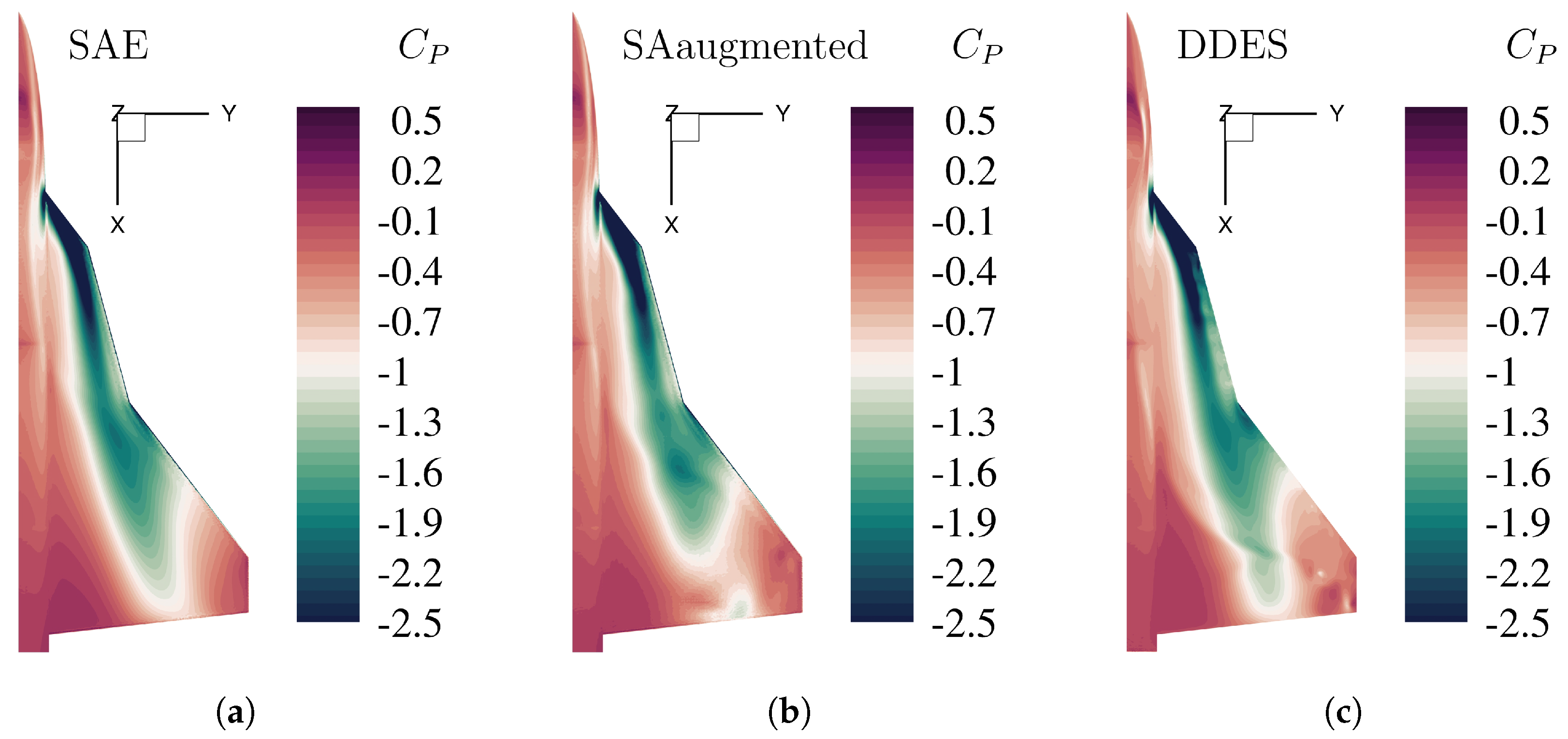
The pressure distribution on the wing suction side for the triple delta wing F3 527552 STLong LV00 SL00 FL00 is depicted in
Figure 8 for the angle of attack
and in
Figure 9 for
. The numerical result corresponding to the original SA model is on the left side of the figures. In the middle subfigure, the results of the augmented enhanced SA model are depicted in the right-hand subfigure numerical results of a high-fidelity delayed Detached Eddy Simulation (DDES) and are shown for reference.
Comparing the two RANS models (
Figure 8a,b), some small changes in the suction peak distribution on the main wing can be seen. The enhanced turbulence model shows lower pressure coefficient values in the front section of the main wing, similar to the high-fidelity DDES results. Looking at
Figure 8 as a reference, the standard turbulence model underestimates the pressure coefficient in the rear part of the main wing, whereas the enhanced turbulence model shows a little higher pressure distribution in this area. Further, the low-pressure area on the strake section caused by the formation of the inboard vortex (IBV) shows a similar downstream distribution for the enhanced model and the DDES, whereas the suction peak for the standard model is further extended downstream from the strake section. The results for
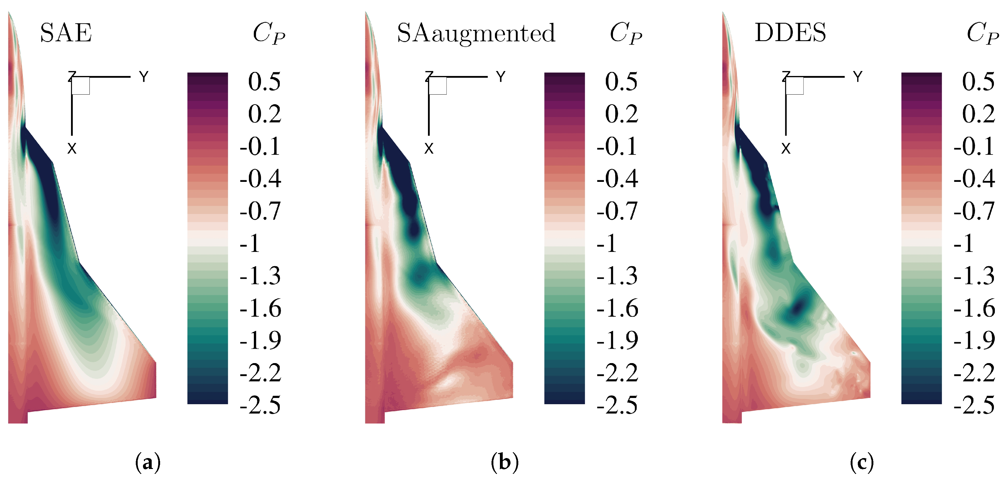
in
Figure 9 show more differences for the different RANS turbulence model than for
in
Figure 8. While the pressure distribution for the standard model in
Figure 9a is very homogenous, the results for the enhanced turbulence model in
Figure 9b display some irregular patterns, with several distinct suction peaks distributed over the whole wing surface. This behavior can also be seen in the high-fidelity DDES result in
Figure 9c. The pressure distribution over the strake section is similar for the enhanced model and the DDES results, where the enhanced turbulence model underestimates the pressure coefficient in the rear part of the strake section before the kink to the main wing section. The DDES result shows only a moderate suction peak in this area, whereas the enhanced turbulence model shows high negative
values. Comparing the main wing section between these two models, the enhanced turbulence model better represents the pressure distribution and the suction peak. While the suction peak is located slightly upstream of the main wing compared to the DDES result, strength, resolution, and distribution are quite similar between the RANS model and the high-fidelity simulation. The different pressure distributions show that the enhanced turbulence model results in a more detailed resolution than the original SA model. While the plots of
in
Figure 8 show slight differences, the plots in
Figure 9 for
show significant differences in pressure distribution over the wing surface. The improved results for the pitching moment coefficient introduced in
Section 7 (
Table 4) are rooted in the enhanced resolution of the adaptive turbulence model.
7.2. Total Pressure Loss
In this subsection, the vortical flow field is analyzed utilizing an isosurface of
total pressure loss
depicted in
Figure 10 for the angle of attack
and for
in
Figure 11. The isosurface is colored in the non-dimensional axial velocity profile
, and stagnating or reversed flow is highlighted by a black isosurface representing areas of
. As in
Section 7.1, results for the numerical results based on the standard SA turbulence model are shown in the left-hand subfigures, and high-fidelity DDES reference results are shown in the right-hand subfigures. The results of the augmented enhanced turbulence model are depicted in the middle subfigures of
Figure 10 and
Figure 11.
Comparing the RANS models in
Figure 10a,b, it can be seen that the adaptive turbulence model shows some vortical flow structure, whereas the standard turbulence model results in a straight smooth isosurface for the total pressure loss. The original turbulence model shows a slightly wider cross-section area of the isosurface over the rear part of the main wing, meaning more total pressure is dissipated by the turbulence model in the flow field compared to the other two models. Focusing on the red spots representing maxima of the non-dimensional axial velocity, it can also be seen that the enhanced turbulence model transports these maxima further downstream, sustaining more energy in the flow field. Although the DDES result in
Figure 10 contains a more detailed resolution, the enhanced turbulence model shows an almost similar distribution of the total pressure loss.
At
the results in
Figure 11 highlight the differences between original and enhanced turbulence models. Neglecting the resolution differences,
Figure 11b shows nearly the same total pressure loss distribution as the high-fidelity DDES result in
Figure 11c. The vortical flow structure and the distribution of the non-dimensional axial velocity are more or less identical, whereas the maxima of non-dimensional axial velocity depicted in red are dissipated approximately at the exact location downstream of the kink between the strake and main wing sections. Vortex breakdown and the irregular flow field are visible over the main wing section for the enhanced turbulence model. The original turbulence model shows a smooth, straight isosurface with no vortical flow structures present. Additionally, it can be seen that the maxima of the non-dimensional axial velocity is dissipated further upstream compared to the other two numerical model.
The results of total pressure loss highlight the different capabilities of vortical flow representation between the original turbulence model and the enhanced turbulence model with additional source terms.
7.3. Normalized Q-Criteria
Another possibility to visualize the rotational flow field is to plot the isosurface of the Q-criterion. A vortex can be defined as a connected fluid region with a positive second invariant of the velocity gradient [
22,
23]. Following Equation (5):
it defines the regions where the vorticity magnitude exceeds the strain-rate magnitude. In
Figure 12 and
Figure 13, the isosurface of the normalized Q-criterion
colorized by the means of total pressure ratio
is shown for the angles of attack
and
, respectively, where
is defined as the mean aerodynamic chord. Additionally, regions of stagnating or reversed flow are marked by a black isosurface representing
.
Comparison of the RANS turbulence models in
Figure 12a,b shows that the normalized Q-criterion for enhanced turbulence model resolves more vortical structures similar to the high-fidelity DDES results in
Figure 12c than the original model. The outboard region of the main wing section especially experiences no vortex flow with the standard turbulence model. Another sign of the improved turbulent diffusion of the enhanced turbulence model is the distribution of the inboard nose vortex. While the nose vortex of the original model is dissolved in the strake section, the nose vortex for the enhanced model extends further downstream and connects with the IBV over the main wing, which can also be seen in the high-fidelity data.
At
in
Figure 13, vortex breakdown is already present, and the standard SA turbulence model fails to resolve any vortical structure exceeding the break-up of the IBV over the strake section. Comparing the three subfigures, it is noticeable that the enhanced turbulence model in
Figure 13b is far more similar to the high-fidelity DDES result in
Figure 13c than to the result of the standard turbulence model. Although vortex breakdown is present, the additional source terms (especially
) enable the turbulence model to resolve the vortex structures in more detail. At this angle of attack, the leading-edge vortex’s strong formation can be seen through a spiral-type vortical structure. High energetic flow, which can be identified by
, is transported further downstream by the enhanced turbulence model. Downstream of vortex breakdown, the RANS model still shows more dissipation, and the vortical structures dissolve totally over the main wing. In contrast, the DDES suggests that the structures exceed the trailing edge.
7.4. Vortex Bursting
The accurate prediction of vortex breakdown and vortex breakdown positions is directly linked to the adverse pressure gradient handling of the turbulence model. Leading-edge vortices experience breakdown at high angles of attack due to the stagnation of the axial core flow caused by the adverse pressure gradient along the vortex core axis [
24]. In the following, the comparison of reversed flow profiles for the three different numerical methods is discussed. In
Figure 14, the results for the angle of attack
are presented, and in
Figure 15, the results for
, respectively. The reversed flow characteristic is analyzed using an isosurface representing regions, where the non-dimensional axial velocity
. The surface distribution for the total pressure ratio
is shown.
Compared to the isosurface of the high-fidelity numerical result in
Figure 14c, it is obvious that the standard SA turbulence model is unable to resolve reversed flow (
Figure 14a). On the other hand, the enhanced turbulence model shows similar reverse flow behavior like the DDES data. Especially the on-set position and downstream extent match the high-fidelity data nearly perfectly.
The same analyses can be carried out for the angle of attack
.
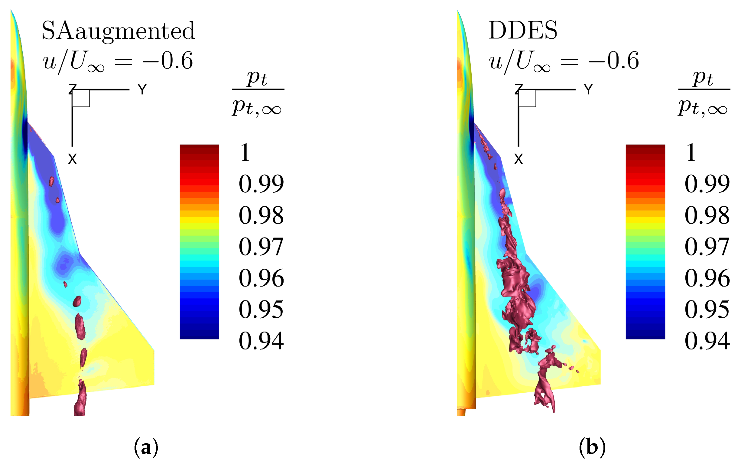
Figure 15 shows that the original turbulence model resolves no reversed flow, while the enhanced turbulence matches the flow characteristics of the high-fidelity results. Although the downstream variation of the isosurfaces cross-section varies differently between these two numerical models, the extent over the whole wing area is present for both models. To better understand the capabilities of the enhanced SA turbulence model, the isosurface of the non-dimensional axial velocity
is shown in
Figure 16 for the angle of attack
. Since in
Figure 15 it is already presented that the original SA model is not capable of resolving this flow characteristic, only the results for the enhanced model and the DDES simulation are presented.
represents regions with strong reversed flow. Comparing the two different numerical approaches, it can be seen that at this magnitude, the RANS model does not represent similar reverse flow structures like the DDES model. This means that the enhanced model shows better resolution capabilities when compared to the original turbulence model but still embodies a higher numerical dissipation than the high-fidelity simulation approach.
In summary, the enhanced turbulence model shows the improved capabilities of reversed flow prediction due to the additional source terms. The proper resolution of this flow feature is important to define the vortex breakdown position and thus properly predict pressure distributions and, as a result, the pitching moment coefficient.
8. Conclusions and Outlook
This study presented the preconditioning capabilities of an HNN framework concerning an adaptive turbulence model based on the standard SA turbulence model. The enhanced turbulence model includes additional source terms linked to a so-called vortex identifier quantity to affect vortex-dominated flow regions only. Model coefficients like those in the original SA model further control the additional source terms. An optimal set of these coefficients can be obtained through an automated optimization process, which needs corresponding computational effort due to the high number of necessary CFD simulations. This work describes the possibility of preconditioning this turbulence model via a machine learning framework rather than relying on the costly optimization procedure. The neural network itself is independent of the underlying input configuration. While the adaptive turbulence model was designed with special emphasis on leading-edge vortex flow systems of medium to low aspect ratio delta wings, the neural network can be fed with any configuration.
The results of the network tests show that the proposed architecture can predict a proper turbulence model coefficient set quite accurately. Most predicted turbulence coefficients are close to their true values, defined by an out-of-the-loop optimization run. The test run also showed that due to the currently available small dataset, the neural network sometimes off-predicts one of the three tested turbulence model coefficients. The reason for this selective misprediction has yet to be found and will be included in future works.
The assessment of improvement is presented employing a comparison of CFD simulation results based on the original SA model, the enhanced SA model, and a high-fidelity DDES simulation. The comparison shows that the enhanced turbulence model with augmented model coefficients improves the resolution of the flow field. Vortical structures, pressure distribution, and reversed flow characteristics are resolved in more detail than for the original turbulence model. The results for the aerodynamic coefficients show that especially the pitching moment coefficient is computed with higher precision due to the improved accuracy in the surface pressure distribution.
In future works, the accuracy of prediction and preconditioning shall be improved by increasing the available training dataset. The dataset and preconditioning framework shall also be tested for different Mach numbers and configurations outside of this work using a generic multiple-swept delta wing platform.
Author Contributions
Conceptualization, M.Z. and C.B.; Methodology, M.Z.; Software, M.Z.; Validation, M.Z.; Formal analysis, M.Z.; Investigation, M.Z.; Resources, M.Z.; Data curation, M.Z.; writing—original draft, M.Z.; writing—review and editing, M.Z. and C.B.; Visualization, M.Z.; Supervision, C.B.; Project administration, C.B.; Funding acquisition, C.B. All authors have read and agreed to the published version of the manuscript.
Funding
The funding of the presented work within the Luftfahrtforschungsprogramm VI-1 (LUFO VI-1) project DIGIfly (FKZ: 20X19091) by the German Federal Ministry for Economic Affairs and Climate Action (BMWK) is gratefully acknowledged.
Data Availability Statement
The data supporting the conclusions of this article will be made available by the authors on request.
Conflicts of Interest
The authors declare no conflict of interest.
References
- Shur, M.L.; Strelets, M.K.; Travin, A.K.; Spalart, P.R. Turbulence Modeling in Rotating and Curved Channels: Assessing the Spalart-Shur Correction. AIAA J. 2000, 38, 784–792. [Google Scholar] [CrossRef]
- Smirnov, P.E.; Menter, F.R. Sensitization of the SST Turbulence Model to Rotation and Curvature by Applying the Spalart–Shur Correction Term. J. Turbomach. 2009, 131, 041010. [Google Scholar] [CrossRef]
- Menter, F.R. Two-equation eddy-viscosity turbulence models for engineering applications. AIAA J. 1994, 32, 1598–1605. [Google Scholar] [CrossRef]
- Arolla, S.K.; Durbin, P.A. Modeling rotation and curvature effects within scalar eddy viscosity model framework. Int. J. Heat Fluid Flow 2013, 39, 78–89. [Google Scholar] [CrossRef]
- Moioli, M.; Breitsamter, C.; Sørensen, K.A. Parametric data-based turbulence modelling for vortex dominated flows. Int. J. Comput. Fluid Dyn. 2019, 33, 149–170. [Google Scholar] [CrossRef]
- Spalart, P.; Allmaras, S. A one-equation turbulence model for aerodynamic flows. In Proceedings of the 30th Aerospace Sciences Meeting and Exhibit, Reno, NV, USA, 6–9 January 1992. [Google Scholar] [CrossRef]
- Duraisamy, K.; Iaccarino, G.; Xiao, H. Turbulence Modeling in the Age of Data. Annu. Rev. Fluid Mech. 2018, 51, 357–377. [Google Scholar] [CrossRef]
- Bengio, Y. Learning Deep Architectures for AI. Found. Trends Mach. Learn. 2009, 2, 1–127. [Google Scholar] [CrossRef]
- Sabater, C.; Stürmer, P.; Bekemeyer, P. Fast Predictions of Aircraft Aerodynamics Using Deep-Learning Techniques. AIAA J. 2022, 60, 5249–5261. [Google Scholar] [CrossRef]
- Zahn, R.; Winter, M.; Zieher, M.; Breitsamter, C. Application of a long short-term memory neural network for modeling transonic buffet aerodynamics. Aerosp. Sci. Technol. 2021, 113, 106652. [Google Scholar] [CrossRef]
- Hitzel, S.M.; Winkler, A.; Hövelmann, A. Vortex Flow Aerodynamic Challenges in the Design Space for Future Fighter Aircraft. In Notes on Numerical Fluid Mechanics and Multidisciplinary Design; Springer: Berlin/Heidelberg, Germany, 2019; pp. 297–306. [Google Scholar] [CrossRef]
- Pfnür, S.; Pflüger, J.; Breitsamter, C. Analysis of Vortex Flow Phenomena on Generic Delta Wing Planforms at Subsonic Speeds. In Notes on Numerical Fluid Mechanics and Multidisciplinary Design; Springer: Berlin/Heidelberg, Germany, 2019; pp. 328–337. [Google Scholar] [CrossRef]
- Hövelmann, A.; Winkler, A.; Hitzel, S.M.; Richter, K.; Werner, M. Analysis of Vortex Flow Phenomena on Generic Delta Wing Planforms at Transonic Speeds. In Notes on Numerical Fluid Mechanics and Multidisciplinary Design; Springer: Berlin/Heidelberg, Germany, 2019; pp. 307–316. [Google Scholar] [CrossRef]
- Guilmineau, E.; Visonneau, M. Evaluation of turbulence modelling for subsonic vortex interaction on multi delta wing configuration. In Proceedings of the 56th 3AF International Conference on Applied Aerodynamics, Toulouse, France, 28–30 March 2022. [Google Scholar]
- Visonneau, M.; Guilmineau, E.; Wackers, J. Computational Analysis of Subsonic Vortex Interaction on Multi Swept Delta Wing Configurations. In Proceedings of the AIAA SCITECH 2022 Forum, San Diego, CA, USA, 3–7 January 2022. [Google Scholar] [CrossRef]
- Schwamborn, D.; Gerhold, T.; Heinrich, R. The DLR TAU-Code: Recent Applications in Research and Industry. In Proceedings of the European Conference on Computational Fluid Dynamics (ECCOMAS CFD 2006), Egmond aan Zee, The Netherlands, 5–8 September 2006; pp. 1–25. [Google Scholar]
- Truesdell, C. The physical components of vectors and tensors. J. Appl. Math. Mech. 1953, 33, 345–356. [Google Scholar] [CrossRef]
- Jeong, J.; Hussain, F. On the identification of a vortex. J. Fluid Mech. 1995, 285, 69–94. [Google Scholar] [CrossRef]
- Nelson, R.C.; Visser, K.D. Breaking Down the Delta Wing Vortex: The Role of Vorticity in the Breakdown Process. In Proceedings of the AGARD Symposium on Vortex Flow Aerodynamics, Scheveningen, The Netherlands, 1–4 October 1990. Ph.D. Thesis Final Report. [Google Scholar]
- Moioli, M.; Breitsamter, C.; Sørensen, K.A. Turbulence Modeling for Leading-Edge Vortices: An Enhancement based on Experimental Data. In Proceedings of the AIAA Scitech 2020 Forum, Orlando, FL, USA, 6–10 January 2020. [Google Scholar] [CrossRef]
- Akiba, T.; Sano, S.; Yanase, T.; Ohta, T.; Koyama, M. Optuna: A Next-generation Hyperparameter Optimization Framework. In Proceedings of the 25th ACM SIGKDD International Conference on Knowledge Discovery and Data Mining, Anchorage, AK, USA, 4–8 August 2019. [Google Scholar]
- Lee, M.J.; Hunt, J.C.R. The structure of sheared turbulence near a plane boundary. In Studying Turbulence Using Numerical Simulation Databases—Ⅱ, Proceedings of the 1988 Summer Program, Stanford, CA, USA, 27 June–22 July 1988; Ames Research Center, National Aeronautics and Space Administration (NASA): Mountain View, CA, USA; Center for Turbulence Research (CTR), Stanford University: Stanford, CA, USA. Available online: https://ntrs.nasa.gov/citations/19890015186 (accessed on 24 January 2024).
- Kolář, V. Vortex identification: New requirements and limitations. Int. J. Heat Fluid Flow 2007, 28, 638–652. [Google Scholar] [CrossRef]
- Mitchell, A.; Molton, P.; Barberis, D.; Delery, J. Characterization of vortex breakdown by flow field and surface measurements. In Proceedings of the 38th Aerospace Sciences Meeting and Exhibit, Reno, NV, USA, 10–13 January 2000. [Google Scholar] [CrossRef]
| Disclaimer/Publisher’s Note: The statements, opinions and data contained in all publications are solely those of the individual author(s) and contributor(s) and not of MDPI and/or the editor(s). MDPI and/or the editor(s) disclaim responsibility for any injury to people or property resulting from any ideas, methods, instructions or products referred to in the content. |
© 2024 by the authors. Licensee MDPI, Basel, Switzerland. This article is an open access article distributed under the terms and conditions of the Creative Commons Attribution (CC BY) license (https://creativecommons.org/licenses/by/4.0/).


