Article

Simultaneous Integration of D-STATCOMs and PV Sources in Distribution Networks to Reduce Annual Investment and Operating Costs

by
Adriana Rincón-Miranda
,
Giselle Viviana Gantiva-Mora
and
Oscar Danilo Montoya
*
Grupo de Compatibilidad e Interferencia Electromagnética (GCEM), Facultad de Ingeniería, Universidad Distrital Francisco José de Caldas, Bogota 110231, Colombia
*
Author to whom correspondence should be addressed.
Computation 2023, 11(7), 145; https://doi.org/10.3390/computation11070145
Submission received: 20 June 2023 / Revised: 11 July 2023 / Accepted: 18 July 2023 / Published: 20 July 2023
(This article belongs to the Special Issue Applications of Statistics and Machine Learning in Electronics)

Abstract

:
This research analyzes electrical distribution networks using renewable generation sources based on photovoltaic (PV) sources and distribution static compensators (D-STATCOMs) in order to minimize the expected annual grid operating costs for a planning period of 20 years. The separate and simultaneous placement of PVs and D-STATCOMs is evaluated through a mixed-integer nonlinear programming model (MINLP), whose binary part pertains to selecting the nodes where these devices must be located, and whose continuous part is associated with the power flow equations and device constraints. This optimization model is solved using the vortex search algorithm for the sake of comparison. Numerical results in the IEEE 33- and 69-bus grids demonstrate that combining PV sources and D-STATCOM devices entails the maximum reduction in the expected annual grid operating costs when compared to the solutions reached separately by each device, with expected reductions of about 35.50 % and 35.53 % in the final objective function value with respect to the benchmark case. All computational validations were carried out in the MATLAB programming environment (version 2021b) with our own scripts.

1. Introduction

1.1. General Context

Medium-voltage distribution networks are infrastructures that span tens or hundreds of kilometers in urban and rural areas in order to supply electricity to all end users while ensuring quality, reliability, efficiency, and security [1]. However, these grids are typically built considering a radial configuration (i.e., a tree structure) [2]. This configuration, although economical from an investment perspective, increases the operating costs, as a radial configuration entails the most significant power losses and low voltage profiles [3]. In terms of percentage, distribution networks typically report losses between 6 to 18%, whereas transmission networks are typically designed to have losses between 1 and 2% [4].
To deal with the higher level of energy losses in distribution networks, distribution companies have implemented different compensation strategies that include shunt reactive power compensation with fixed and step variable capacitor banks [5], static distribution compensators (D-STATCOMs) [6], flexible AC transmission systems (FACTS) [7], grid reconfiguration [8], and active power compensation via distributed generation sources [9], among others. All of these compensation strategies have proven to be effective in grid operation (i.e., in the reduction of energy losses and purchasing costs, as well as in voltage profile improvements). However, dispersed generation is an expensive solution to deal with energy losses when compared to reactive power compensation [6].

1.2. Motivation

Considering the alternatives available for improving the electrical performance of medium-voltage distribution networks, this research aims at the effective integration of PV generators and D-STATCOMs to minimize the expected energy purchasing costs at the terminals of the substation for a projected planning period [10]. The use of PV generation allows indirectly reducing CO 2 emissions by reducing the energy generated at the substation, which is equivalent to avoiding the use of conventional thermal sources to produce electricity [11]. In addition, using D-STACOMs in distribution networks helps to reduce the total grid power losses and improve voltage profiles, which generally makes distribution networks more efficient and reliable [12]. The main idea of this research is to explore the separate and simultaneous integration of both compensation devices. However, the mathematical formulation involved belongs to the family of mixed-integer nonlinear programming (MINLP) models, which implies that it is not possible to ensure a global optimum [13]. Therefore, this research is also motivated by the idea of proposing a leader-follower optimization methodology that allows dealing with the optimal sizes and locations of these devices in medium-voltage distribution networks that is efficient and has low computational complexity due to its sequential programming structure.

1.3. Literature Review

The problem regarding the optimal integration of PVs and D-STATCOMs in medium-voltage distribution networks has been widely explored in the specialized literature, mainly focusing on the separate integration of each device, i.e., the allocation and sizing of PVs or D-STATCOMs without simultaneous analysis. Some of the most recent advances in this research area are presented below.
The authors of [14] presented the application of the vortex search algorithm (VSA) to address the problem regarding the efficient integration of PV systems in electrical distribution networks, considering the possibility of operating with both AC and DC distribution technologies, which improved the results reported in [4], where only AC grids where analyzed. The main goal of PV integration was to minimize the network’s equivalent investment and operating costs. Numerical results in the IEEE 33- and 69-bus grids demonstrated the effectiveness of the proposed optimization approach when compared to the discrete-continuous version of the vortex search algorithm.
In [15], the authors presented a general literature review regarding the integration of renewable generation in electrical networks. They demonstrated that these technologies are the essential driver for improving the quality of the energy service, and they studied economic and atmospheric parameters. A complete review of the most common optimization methods based on metaheuristics was provided, where classical methods such as particle swarm optimization, genetic algorithms, and ant-lion optimizers were analyzed.
The work by [16] presented a heuristic analysis based on multiple simulations run in the DIgSILENT software to determine an adequate renewable energy penetration based on PV generation sources, with the aim to minimize the expected grid energy losses. Numerical results in the IEEE 13-, 33-, and 34-bus grids, among others, demonstrated that the proposed approach indeed allowed identifying the degree of PV penetration and the potential nodes for installation.
The authors of [17] presented a complete review of the state of the art on the efficient integration of PV systems in electrical distribution grids. The main contribution of this research was that it identified the most suitable programming models for integrating renewables in electrical grids while considering the constraints, possible objective functions, and applicable solution methodologies.
Additional solution methodologies applicable to the efficient integration/operation and control of PV systems in electrical networks include the particle swarm optimization algorithm [18,19], the tabu search algorithm [20], the krill heard optimizer [21], the bat optimization algorithm [22], and the wild horse optimization approach [23,24], among others.
As for the efficient integration of D-STATCOMs, some of the most recent approaches reported in the specialized literature are the following.
The authors of [6] applied the VSA approach to locate and size D-STATCOMs in distribution networks. Their objective function was the minimization of the annual operating costs of the network for a period of one year. These costs included the costs of energy losses and the investments made in D-STATCOMs. Numerical results demonstrated the effectiveness and robustness of this approach in comparison with the exact solution of the MINLP model reached by the GAMS software.
The work by [25] presented the application of the sine-cosine algorithm to define the location and size of D-STATCOMs in distribution networks with a radial topology. A multi-objective analysis showed that this approach minimizes the total grid power losses, improves the voltage grid profile, and increases the grid stability index. Numerical comparisons with the classical particle swarm optimization method demonstrated the effectiveness of the proposed optimization model.
In [26], the problem regarding the efficient integration and dispatch of D-STATCOMs in distribution networks was addressed via convex optimization while including a stochastic analysis. Numerical results in the IEEE 33- and 69-bus grids improved the numerical results reached by solving the exact MINLP model in the GAMS software.
The authors of [12] presented a complete review of the literature on the optimal placement and sizing of D-STATCOMs for distribution system applications. This document reviews the objective functions considered (technical or economic) and the classical solution methodologies, which include sensitive-based algorithms, combinatorial optimizers, and convex approaches.
Regarding the simultaneous integration of PVs and D-STATCOMs, the authors of [9] presented the combination of these devices in a new technology known as PV-STATCOMs, which consists of adding reactive power control capabilities to the voltage source inverters that interface the PV systems with the electrical network. Recently, the study by [27] applied the hunter-prey-based algorithm to locate and size PV-STATCOMs in medium-voltage distribution networks, in order to minimize the expected grid power losses and improve the average grid voltage profile. Numerical results in the IEEE 33-bus grid showed the efficiency and robustness of the proposed algorithm when compared to different combinatorial optimizers.
The above-presented literature review allows noting two main aspects: (i) the integration of PVs and D-STATCOMs is a research area of high interest for industry and academia, as these devices allow improving the technical, economic, and environmental aspects of distribution grids; and (ii) most optimization methodologies are based on combinatorial algorithms, which confirms that these are well-established methods which provide efficient solutions to complex MINLP formulations, as is the case of this research.

1.4. Contribution and Scope

Considering the above, the main contributions of this research article are the following:
  • A general MINLP formulation of the problem regarding the simultaneous integration of PVs and D-STATCOMs in medium-voltage distribution networks in order to minimize the expected annual grid investment and operating costs while considering variable active and reactive power demand curves. This formulation is based on the combinations existing in the literature for the efficient, independent integration of each device.
  • The application of a leader-follower optimization methodology based on hybridizing the VSA and the successive approximations power flow method. Based on the VSA approach, the leader stage uses a discrete continuous-codification vector to define the nodes where the PVs and D-STATCOMs must be placed (discrete part) and their optimal sizes (continuous part). On the other hand, the follower component of the optimization approach is associated with the technical evaluation of each solution provided by the leader, i.e., the calculation of voltages and powers, among other variables.
Numerical results in the IEEE 33- and IEEE 69-bus grids demonstrate that the simultaneous integration of PVs and D-STATCOMs is the best option to minimize the expected investment and operating costs of a network for a planning period of 20 years. This, in comparison with the separate integration of each device.
It is worth mentioning that, in the scope of this research, the following aspects are considered: (i) the daily active and reactive power demand curves, as well as the solar availability in the area of influence of the distribution networks, are considered exogenous inputs provided by the distribution company, which implies that these are regarded as constant data during the solution process of the MINLP model (i.e., they have no uncertainties); and (ii) the selection of the VSA combined with the successive approximation power flow method for the leader-follower optimization strategy was based on the excellent results reported in the specialized literature for separately integrating PVs [4,14] and D-STATCOMs [6].

1.5. Document Structure

The remainder of this research is structured as follows. Section 2 presents the mathematical model of the problem aimed at locating and sizing PV systems and D-STATCOMs (both separately and simultaneously). Section 3 shows the main characteristics of the leader-follower optimization technique, where the leader algorithm corresponds to the vortex search algorithm (VSA) with a discrete-continuous codification, and the follower algorithm is the classical successive approximations power flow method. Section 4 outlines the main details of the IEEE 33- and 69-bus grids, the active and reactive power curves, and the solar generation availability. Section 5 describes the main numerical results of the studied problem while considering four simulation scenarios, which include a benchmark case and the separate and simultaneous integration of PVs and D-STATCOMs. Finally, Section 6 presents the main concluding remarks of this research, as well as possible future works.

2. Mathematical Model

This section presents the mathematical formulation of the studied problem, which is presented in three parts: the problem regarding the optimal placement and sizing of PV sources, the same problem for D-STATCOMs, and the combination of both models, i.e., the simultaneous allocation of PV generators and D-STATCOMs.

2.1. Mathematical Model for Locating and Sizing PV Generation Units

2.1.1. Objective Function Formulation

The main idea when it comes to optimally integrating renewable energy resources based on PV systems in electrical distribution networks is to minimize the expected operating f 1 and investment f 2 costs during a project. This objective function is formulated in Equation (1) [17].
min A cost 1 = f 1 + f 2
where the components f 1 and f 2 are defined in Equations (2) and (3).
f 1 = C k W h T f a f c h ϵ H i N p i , h c g Δ h
f 2 = C p v f a i ϵ p v p i p v + T h ϵ H i ϵ p v C O & M p v p i , h p v Δ h
Here, f 1 is the function that allows finding the annual costs of the purchase or production of the energy produced by the conventional generators installed in the electrical network during the useful life of the distributed PV systems; C k W h is the average cost of energy purchasing at the substation bus; T is the number of days in a year (i.e., 365 days); p i , h c g represents the active power generation in the slack bus connected at node i at time h; Δ h is the division time used for representing data during a day of operation (typically 1 h, 0.5 h, or 0.25 h); f 2 is a function that allows calculating the annualized investment costs associated with the installation and maintenance of the PV generation units in the electrical grid; C p v denotes the installation costs of the PV plants per unit of capacity (USD/kWp); p i p v is the size of the PV generation installed; and C O & M p v represents the average maintenance and operation costs of the PV sources. Note that H , N , and T are the sets containing the daily periods, the number of nodes, and the number of years analyzed, respectively. In addition, the factors f a and f c are defined below.
f a = t a 1 ( 1 + t a ) N t ,
f c = t ϵ T 1 + t e 1 + t a t ,
where f a is the annualization cost factor; f c is the projection of the expected energy purchasing costs during the project; t a represents the fixed rate of return for the investments made by the owner or operator of the network during the planning horizon; N t is the number of years of the project; and t e represents the percentage increase regarding the costs of energy purchasing during the planning horizon, which corresponds to 20 years.

2.1.2. General Set of Constraints

The problem regarding the optimal location and sizing of PV plants in electrical distribution networks implies some typical constraints associated with the active and reactive power balance, voltage regulations, and device capabilities, among others. The complete set of constraints is presented below.
p i , h c g + p i , h p v P i , h d = v i , h j N Y i j v j , h c o s ( θ i , h θ j , h φ i j ) , i N & h H
q i , h c g Q i , h d = v i , h j N Y i j v i , h s i n ( θ i , h θ j , h φ i j ) , i N & h H
P i c g , min p i , h c g P i c g , max , i N & h H
Q i c g , min q i , h c g Q i c g , max , i N & h H
x i p v P i , h p v , min p i p v x i p v P i , h p v , max , i N
p i , h p v = G i , h p v p i p v , i N
v min v i , h v max , i N & h H
i N x i p v N p v a v a
Equation (6) defines the active power balance, where P i , h d represents the active power demanded at node i and time h; V i , h and V j , h correspond to the voltage magnitudes at nodes i and j at time h, whose angles are θ i , h and θ j , h , respectively; and Y i j and φ i j are the magnitude and angle of the components of the admittance matrix that relates nodes i and j, respectively. Equation (7) defines the reactive power balance per node and period, with Q i , h d being the power demanded at node i in period h, and q i , h c g the reactive power injection in the conventional generator connected at node i and time h. In (8), the parameters P i c g , min and P i c g , max define the lower and upper bounds for active power generation in the conventional source, while, in (9), Q i c g , min and Q i c g , max correspond to the upper and lower bounds for reactive power generation by the conventional generator connected at node i. Inequality constraint (10) defines the lower and upper bounds of active power generation at node i and time h, i.e., P i , h p v , min and P i , h p v , max , when the binary variable x i p v is activated. Equation (11) defined that the PV generation sources must operate with maximum power point tracking, which implies that each generator will follow the generation availability curve G i , h p v . Inequality constraint (12) defines the admissible voltage regulation bounds for the voltage profiles in all nodes and periods, with v min and v max being the minimum and maximum voltage limits. Finally, inequality constraint (13) defines the maximum number of PV generators available for installation (i.e., N p v a v a ) in the entire distribution grid.
The parameterization of the optimization model (1)–(13) is presented in Table 1.

2.2. Mathematical Model for Locating and Sizing D-STATCOMS

2.2.1. Objective Function Formulation

The problem regarding the optimal siting and sizing of D-STATCOMs in medium-voltage distribution networks can be modeled as a MINLP model, where the binary variables correspond to the nodes where the reactive power compensators must be installed and the continuous part is associated with the power flow variables, i.e., voltages and powers. The objective function of this problem is presented in (14).
min A cost 2 = f 1 + f 3
where f 3 is the component of the objective function associated with the annualized investment in D-STATCOMs.
f 3 = γ i N ω 1 ( q i c o m p ) 2 + ω 2 q i c o m p + ω 3 q i c o m p ,
where q i c o m p is the installed capacity of the D-STATCOM connected at node i; ω 1 ω 2 , and  ω 3 are the cubic, quadratic, and linear objective function coefficients [28], with γ being the annualization factor applied to the investment costs in D-STATCOMs while considering a useful life of 20 years [29].

2.2.2. General Set of Constraints

This problem implies some typical constraints associated with the active and reactive power balance, voltage regulations, and device capacities, among others. The complete set of constraints is presented below.
p i , h c g P i , h d = v i , h j N Y i j v j , h c o s ( θ i , h θ j , h φ i j ) , i N & h H
q i , h c g + q i , h c o m p Q i , h d = v i , h j N Y i j v i , h s i n ( θ i , h θ j , h φ i j ) , i N & h H
P i c g , min p i , h c g P i c g , max , i N & h H
Q i c g , min q i , h c g Q i c g , max , i N & h H
x i c o m p Q i c o m p , min q i c o m p , max x i c o m p Q i , h c o m p , max , i N
q i , h c o m p = q i c o m p , i N
v min v i , h v max , i N & h H
i N x i c o m p N c o m p a v a ,
Equation (16) defines the active power balance per node and period. Equation (17) presents the reactive power balance per node and period, with q i , h c o m p being the hourly reactive power injection at the D-STATCOM connected at node i. Inequality constraints (18) and (19) express the limitations regarding active and reactive power generation applied to the conventional source connected at node i. Inequality constraint (20) presents the maximum and minimum sizes applicable to the D-STATCOM that to be connected at node i, i.e., Q i c o m p , max and Q i c o m p , min , if the binary variable x i c o m p is activated. Equation (21) shows that the D-STATCOMs are designed to inject constant reactive power during all periods. Inequality constraint (22) presents the upper and lower bounds applicable to voltage operation along the distribution grid. Finally, inequality constraint (23) defines the maximum number of reactive power compensators available for installation (i.e., N c o m p a v a ).
The parameterization of the optimization model (14)–(23) is presented in Table 2.

2.3. Mathematical Model for Simultaneously Locating and Sizing PV Generation Units and D-STATCOMs

2.3.1. Objective Function Formulation

The objective function considered for this work corresponds is a combination of those presented in Section 2.1 and Section 2.2, with the aim to minimize the annual operating costs of the electrical grid over 20 years. This objective function is presented in Equation (24).
min A cost 3 = f 1 + f 2 + f 3
According to the explanations provided in the previous sections, f 1 is used to determine the annual production or acquisition costs of energy generated by conventional generators, and f 2 allows calculating the annual investment costs associated with installing and maintaining photovoltaic (PV) generation units. Finally, f 3 is related to the annualized investment costs of D-STATCOMS. The 20-year planning horizon has been previously considered in the values of the constants presented in Table 1 and Table 2, as well as in the annualization factors f a and f c .

2.3.2. General Set of Constraints

The problem regarding the simultaneous optimal location and sizing of PV units and D-STATCOM devices in distribution networks involves several constraints. The complete set of constraints is presented below:
p i , h c g + p i , h p v P i , h d = v i , h j N Y i j v j , h c o s ( θ i , h θ j , h φ i j ) , i N & h H
q i , h c g + q i , h c o m p Q i , h d = v i , h j N Y i j v i , h s i n ( θ i , h θ j , h φ i j ) , i N & h H
P i c g , min p i , h c g P i c g , max , i N & h H
Q i c g , min q i , h c g Q i c g , max , i N & h H
x i p v P i , h p v , min p i p v x i p v P i , h p v , max , i N
x i c o m p Q i c o m p , min q i c o m p , max x i c o m p Q i , h c o m p , max , i N
p i , h p v = G i , h p v p i p v , i N
q i , h c o m p = q i c o m p , i N
v min v i , h v max , i N & h H
i N x i p v N p v a v a ,
i N x i c o m p N c o m p a v a ,
For the simultaneous model, the equations for the active (25) and reactive power balance (26) should include the active power generated by the PV units and the reactive power delivered by the D-STATCOMS. The inequalities that relate to the upper and lower limits of active (27) and reactive power (28) for the conventional generators and the network voltage (33) generally depend on the network conditions. Therefore, they apply without changing the D-STATCOMS and the PV units. The inequalities associated with the limits of PV generation (29) and power injection of the D-STATCOMS (30), those relate production to h periods ((31) and (32)), and the available amount of devices for installation ((34) and (35)) all depend individually on the conditions of each PV system or D-STATCOM.
This mathematical model does not have a linear structure due to the trigonometric functions and voltage products that are implicitly present in the equations of active and reactive power balance. This implies a complex solution with conventional optimization methods. Therefore, convex optimization or combinatorial tools may be suitable. This research focuses on applying an efficient combinatorial optimization method with a classical power flow tool to solve the exact MINLP model via a leader-follower methodology.

3. Proposed Leader-Follower Optimization Approach

A leader-follower optimization methodology is proposed to deal with the problem under study. The leader strategy uses a discrete codification to determine the value of the binary variables x i c o m p and x i p v , in addition to a continuous codification part that defines the sizes of these systems. In the follower stage, a conventional multi-period power flow formulation is implemented to evaluate the system’s operating costs, i.e., the energy purchasing costs at the terminals of the substation. The main characteristics of the leader-follower optimization strategy are presented below.
  • In the leader stage, a combinatorial optimization method is implemented to evolve an initial set of individuals, i.e., a set of a potential solutions, where the discrete codification implemented allows evaluating the components f 2 and f 3 regarding the installation costs of the PV and D-STATCOM systems.
  • The follower stage determines the expected energy purchasing costs at the terminals of the substation (i.e., f 1 ) and the operating and maintenance costs of the PV systems.
The main characteristics of the leader and follower components of the proposed solution methodology are detailed below.

3.1. Follower Stage: Successive Approximations Power Flow Method

In optimization approaches involving electrical distribution networks and their technical characteristics, such as voltage and power calculations, a follower stage requires the recursive solution of the power flow problem for a single or multi-period analysis [30]. In the case of distribution networks, the most common power flow methodologies are based on graph-based methods, i.e., they exploit the grid topology, typically radial or weakly meshed, in order to propose efficient iterative formulas [31,32]. This research adopts one of the most efficient power flow methods for distribution networks, which was originally proposed by the authors of [33], known as the successive approximations power flow method.
The general power flow formula of the successive approximations power flow method in the complex variable domain is presented in (36). This iterative formula allows solving the active and reactive power flow equations defined by (28) and (29).
V d h m + 1 = Y d d 1 diag 1 V d h m , S d h S c o m p h S p v h + Y d g V g h , h H
where m corresponds to the iterative counter; V d h represents a complex vector that contains the voltage variables per period of analysis in all the nodes of the network; V g h is the vector associated with the fixed voltage output at the terminals of the substation; Y d d is an invertible matrix that contains the admittance relations between the demand nodes; Y d g represents a rectangular matrix associating the admittances between the substation bus and the demand nodes; S d h represents the vector that contains the constant power consumptions per period of analysis; and S c o m p h and S p v h represent vectors that contain the apparent power injection in the reactive power compensators and PV generation systems installed along the distribution grid. · corresponds to the conjugate operation associated with the complex variable inside the parenthesis.
Note that the initialization of the power flow Formula (36) requires defining the voltage values of the demand nodes at t = 0 (i.e., V d h 0 V g h ), which are assigned as equal to the substation voltage.
Remark 1.
The convergence of the recursive power flow formula defined in (36) can be demonstrated by applying the Banach fixed-point theorem, as demonstrated by the authors of [33]. In addition, the values associated with the apparent power injection in the D-STATCOM and PV systems (see vectors S c o m p h and S p v h ) are provided by the leader stage and define the intrinsic relation between the leader and the follower optimization layers. Therefore, the follower stage is considered to be the heart of leader-follower optimization algorithms [34].
The following stopping criterion is applied to ensure that the recursive power flow formula in (36) reaches the desired convergence.
max h H V d h m + 1 V d h m ϱ ,
where ϱ represents the maximum tolerance, typically defined as 1 × 10 10 [33].
Once the power flow formula in (36) has reached the desired convergence, the power generation at the substation source can be determined as presented in (38).
S g h = Y g g V g h + Y g d V d h
which allows calculating the component of the objective function f 1 , as presented in Equation (39).
f 1 = C k W h T f a f c h H real S g h ,

3.2. Master Stage: The Vortex Search Algorithm (VSA)

The VSA is a combinatorial methodology from the family of physics-inspired optimization algorithms, which was developed in 2015 by the authors of [35]. This algorithm aims to emulate the physical behavior of the vortical flow of stirred fluids using a Gaussian formulation structure [36]. The VSA is an optimization method developed for continuous optimization problems that balance the exploration and exploitation stages by considering hyper-ellipses with a variable radius that initially cover all of the solution space [37]. During the iterative process, the hyper-volume of this hyper-ellipse is reduced in order to explore specific, promising areas of the solution space. This exploration and exploitation is performed using a Gaussian distribution and incomplete gamma functions [35]. Even though the VSA was initially designed for continuous optimization problems, it can be adapted to discrete-continuous problems, as proposed in [14]. Thus, the VSA can deal with the simultaneous placement and sizing of PV and D-STATCOMs in distribution networks.

3.2.1. Generating the Initial Solution

To generate the initial solution as per the VSA approach, consider a multi-dimensional space with size d. In addition, the main characteristic of the VSA is that it generates a hyper-ellipse centered at the solution space in the first iteration (i.e., t = 0 ), whose radius r t is continuously reduced as the iterative process advances. The the initial center of the hyper-ellipse is defined in (39).
μ 0 = x min + x max 2 ,
where x min R d × 1 and x max R d × 1 are the lower and upper bounds of the decision variables.
Remark 2.
Considering that the VSA approach will determine the nodes for locating PV and D-STATCOM systems, the discrete component of μ 0 , i.e., its first d / 2 positions, must be rounded to ensure the feasibility of the solution space, given that the nodes of electrical distribution networks are typically represented as integer numbers.

3.2.2. Generating the Candidate Solutions

To obtain a set of candidate solutions C i t ( x ) = s i t = x 1 , x 2 , , x d , with i being a sub-index related to the ith potential solution individual contained in the population. As proposed by the authors of [35], the generation of candidate solutions is reached by implementing a Gaussian distribution with the structure presented in (41).
s i t = p ζ i t , μ t , v = 2 π d v 1 / 2 e 1 2 ζ i t μ t v 1 ζ i t μ t .
In this distribution probability, ζ i t R d × 1 corresponds to a vector containing random numbers with appropriate dimensions, μ t R d × 1 corresponds to the current center of the hyper-ellipse at iteration t, and v R d × d is known as the covariance matrix. The work by [36] recommends simplifying this matrix by considering equal variances in its diagonal and null covariances. This simplification can be formulated as follows:
σ 0 = max x max min x min 2 ,
where v is defined as σ 0 I d × d , considering that I is an identity matrix with dimensions d × d .
Remark 3.
At the beginning of the optimization process, the authors of [35] suggest that the initial radius r t of the hyper-ellipse be selected as equal to σ 0 when t = 0 . This selection is supported by the idea that, during the initial evolution of the VSA approach, the hyper-ellipse must cover the entirety of the hyper-volume of the solution space, which implies that its initial radius must be as large as possible. This radius will decrease as the iteration process advances, since the VSA will transition from the exploration to the exploitation stage, where promising regions of the solution space will be checked.
Note that the reduction of the radius will affect the generation of random values in the ζ i t vector, as ζ i t = r t rand d , where rand d defines a generation of values 0 and 1 with dimension d following a uniform distribution.

3.2.3. Correcting the Candidate Solutions

Given the random nature of the evolution process in all combinatorial optimization methods, including the VSA approach, each s i t may have values outside of the limits of the solution space, which makes them impossible to evaluate in the follower stage [14]. Therefore, in this kind of method, each and every candidate solution must be evaluated [17]. In this work, each potential solution s i t is checked as presented in (43).
s i , j t = s i , j t x j min x j x j max , j = 1 , 2 , , d x j min + x j max x j min rand ( 1 ) otherwise , j = 1 , 2 , , d
where rand ( 1 ) is a random number between 0 and 1, generated with a uniform distribution. Note that, once all solution individuals have been evaluated, the first d / 2 part is rounded to the nearest integer in order to ensure that the location of the PV and D-STATCOM systems is feasible.
To illustrate the general structure of a potential solution individual s i t , consider the vector defined below.
s i t = x k p v x l c o m p p k p v q l c o m p [ 12 , k , , 30 21 , 9 , , l 0.1897 , p k p v , , 1.3801 0.1624 , 0.5598 , , q l c o m p ]
which is a discrete-continuous codification, where the first d / 2 positions denote the nodes for locating PV units and D-STATCOMs and the second part is associated with their sizes.

3.2.4. Selecting the New Hyper-Ellipse Center

The evolution of the VSA through the solution space is governed by the location of the hyper-ellipse center, which corresponds to the best current individual contained in the set of candidate solutions C i t ( x ) , i.e., μ t + 1 = s i , best t [35]. It is worth mentioning that the best current solution will depend on the nature of the optimization problem, which, in this case, is the candidate with the lowest objective function value. Otherwise, it will correspond to the potential solution individual with the highest objective function value [4].

3.2.5. Radius Reduction Criterion

To transition from the exploration to the exploitation stage in the VSA, a reduction of the radius of the hyper-ellipse is performed in each iteration. In the specialized literature, there are two ways to implement this reduction. In the original version of the VSA approach, which was presented by [35], an incomplete inverse gamma function was reported. However, the study by [4] proposed an exponential rule. This work employed the latter since its computational implementation is simple and efficient. This reduction rule is defined in (44).
r t + 1 = σ 0 1 t t max e 6 t t max ,
with t max being the maximum number of iterations assigned to the optimization algorithm.

3.2.6. Stopping Criteria

The exploration and exploitation of the solution space using the VSA ends
if the maximum number of iterations t max is reached, or
if, after τ max consecutive iterations, the center of the hyper-ellipse has not been modified.

3.3. General Implementation of the Proposed Leader-Follower Optimization Algorithm

The application of the VSA approach to the problem regarding the simultaneous location and sizing of PV units and D-STATCOMs in distribution networks is presented in Algorithm 1 [4].
Algorithm 1: Application of the VSA approach for locating and sizing PVs and D-STATCOMs in distribution networks.
Data: Read data of the distribution network under analysis
Obtain the per-unit equivalent of the distribution network;
Define the initial center and radius of the hyper-ellipse μ t and r t ;
Generate the initial set of candidate solutions s i t using (41);
Check and correct each potential solution s i t using (43);
Evaluate each potential solution s i t in the follower stage, i.e., the power flow
  formula defined in (36);
Find the best current solution s i , best t ;
for  t = 1 : t max  do   
    Update the hyper-ellipse center making μ t + 1 = s i , b e s t t ;   
    Calculate the new radius of the hyper-ellipse r t + 1 as in (44);   
     Generate the new set of candidate solutions s i t using (41);   
      Check and correct each potential solution s i t using (43);   
     Evaluate each potential solution s i t in the follower stage, i.e., the power flow   
        formula defined in (36);   
      Find the best current solution s i , best t ;   
      if  τ τ max  then 
        Report the best current solution in μ t + 1
        break;
    end   
end
Result: Return the best solution found

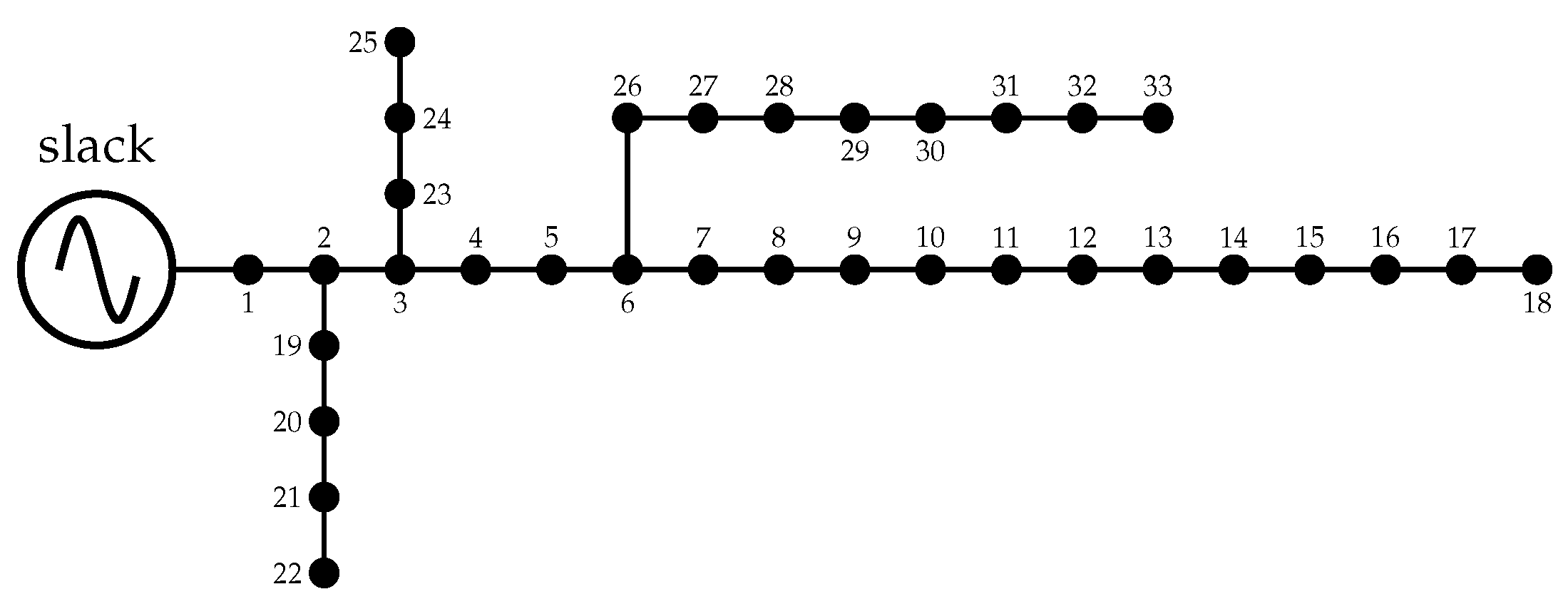
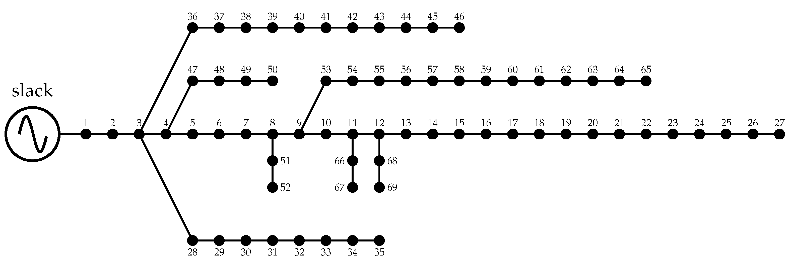
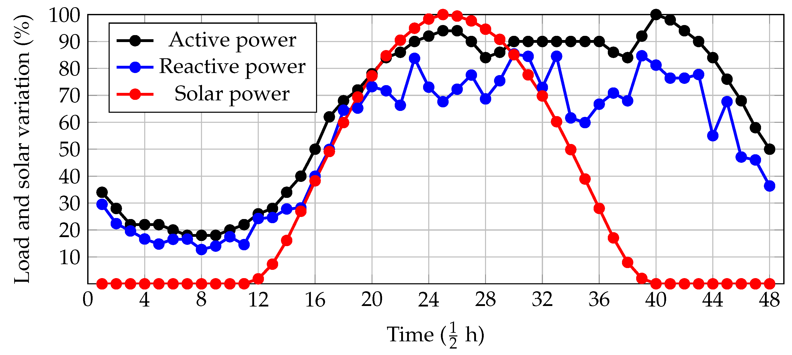
4. Test Feeder Characterization

To validate the effectiveness and robustness of the proposed leader-follower optimization methodology to locate and size PV units and D-STATCOMs in medium-voltage distribution networks, the IEEE 33- and 69-bus grids were used as test feeders. The schematic nodal connection of these feeders is presented in Figure 1 and Figure 2, and their electrical parameters regarding branches and peak load consumptions are listed in Table 3 and Table 4. Note that the main characteristics of these test feeders are their radial structure and their voltage profile, which is equal to 12.66 kV at the terminals of the substations located at node 1 in both cases. In addition, the voltage regulation bounds were assigned as ± 10 % .
To define the expected behavior of the electrical distribution network for the planning period, the solar availability and the active and reactive power consumptions in the area of influence of the studied distribution network are presented in Figure 3.

5. Numerical Results

For the computational implementation of the proposed leader-follower optimization approach, the MATLAB software (version 2021b) was employed on a PC with an AMD Ryzen 7 3700 2.3 GHz processor and 16.0 GB RAM running a 64-bit version of Microsoft Windows 10 Single Language. The VSA and the successive approximations power flow method were executed with our own scripts. The following simulation scenarios were evaluated for each test feeder.
S1.
The evaluation of a benchmark case, i.e., the original conditions of the test feeder without including PVs and D-STATCOMs.
S2.
The solution of the optimization model (14)–(23), which corresponds to the optimal location of D-STATCOMs in distribution networks.
S3.
The solution of the optimization model (1)–(13), which corresponds to the optimal location of PV plants in distribution networks.
S4.
The solution of the optimization model (24)–(35), i.e., the simultaneous location of PV units and D-STATCOM systems in distribution networks.
It is worth mentioning that, in the parameterization of the VSA approach, 10 solution individuals in the population were considered, as well as 1000 iterations and 100 evaluations of the whole optimization strategy. In addition, for the successive approximations power flow method, 100 iterations and a tolerance equivalent to 1 × 10 10 were assigned.

5.1. Numerical Results for the IEEE 33-Bus Grid

Table 5 reports the numerical solutions reached with the proposed leader-follower optimization algorithm in the IEEE 33-node system.
These results show that:
  • In S2, three D-STATCOMs with sizes of about 186.4, 121.1, and 528.6 kvar were placed at nodes 14, 25, and 30. With these devices, a reduction of about USD 22,602.85 in the expected grid operating costs corresponds to 0.64 % . However, this is an expected result, as the D-STATCOMs provide reactive power and the energy purchasing costs at the terminals of the substation are associated with active power. This implies that the utility company must purchase less energy to support all the end users since the D-STATCOMs improve the grid efficiency.
  • As expected, in S3, a reduction of about USD 1,252,832.78 (i.e., 35.26 % with respect to the benchmark case) in the total grid costs was achieved by installing three PV generators at nodes 10, 16, and 32, with sizes of about 833.7, 918.5, and 1668.4 kW. This significant reduction in the objective function calue can be attributed to the fact that the PV generators provide active power to all the energy sources during the part of the day that has adequate solar radiation, which means that the substation bus reduces its active power injection, i.e., less energy must be purchased in the spot market to supply the end users, which is directly related to the final value of the objective function.
  • The combination of D-STATCOMs and PV sources in S4 shows different locations and sizes when compared to the individual solutions in S2 and S3. Nevertheless, the joint use of these devices allowed for a reduction of about USD 1,261,534.76 (i.e., 35.50 ) in the objective function with respect to the benchmark case. This was achieved by installing 3375.8 kW in PV sources and 798.4 kvar in D-STATCOMs, which confirms that, with the simultaneous integration of these devices, the best objective function value is reached, with reduced sizes in the D-STATCOMs and PV sources, when S4 is compared against S2 and S3, i.e., 836.1 kvar and 3420.6 kW.
As for the processing times required to reach the solutions in Table 5, it was observed that, after 100 consecutive evaluations, S2 took 61.71 s, S3 about 61.81 s, and S4 79.88 s, which demonstrates that an efficient solution for integrating PV units and D-STATCOMs in medium-voltage grids can be reached in less than two minutes. This time can be considered to be low, taking into account that the dimension of the solution space is infinite due to the presence of continuous variables in the optimization model, with thousands of binary combinations in each case of nodal selection.

5.2. Numerical Results for the IEEE 69-Bus Grid

Table 6 reports the numerical solutions reached with the proposed leader-follower optimization algorithm in the IEEE 69-bus system.
These results show that:
  • The installation of D-STATCOMs in S2 allowed for an effective reduction of about USD 25,629.68 in the objective function value, i.e., 0.69 % with respect to the benchmark case. This result confirms (as happened with the IEEE 33-bus grid) that the D-STATCOMs contribute to minimizing the expected grid power losses, which in turn reduces the energy purchased at the terminals of the substation and therefore the total operating costs.
  • In S3, the use of PV systems showed an effective reduction of about 35.36 % in the total grid operating and investment costs with respect to the benchmark case, which confirms that PV plants indeed allow distribution companies to reduce the expected energy purchasing costs (by about USD 1,316,577.62 ).
  • The combination of PV units and D-STATCOMs in S4 showed the most efficient reduction in the total grid operational cost, with a reduction of about USD 1,323,038.87 , i.e., a 35.53 % improvement with respect to the benchmark case. This demonstrates that, for utility companies, this approach constitutes an efficient option to reduce their operating costs and improve their grid efficiency in the form of reduced total grid energy losses, which indirectly improves the grid voltage profile.
Regarding processing times, it is worth mentioning that, in S1, the average processing time for defining the location and sizing of D-STATCOMs was about 269.14 s, in S3, this time was about 271.41 s, whereas, in S4, the average time was about 336.01 s. Thus, the solution to the studied problems in the IEEE 69-bus grid took less than 6 min, which is a very low value considering that the dimension of the solution space is infinite for each combination of binary variables (i.e., the nodes where the D-STATCOMs and PV units must be placed).

6. Conclusions and Future Work

The problem regarding the efficient integration of PV plants and D-STATCOMs in electrical networks was addressed in this research by applying a leader-follower optimization strategy. In the leader stage, using a discrete-continuous codification, the VSA approach was implemented to determine the optimal location of PV systems and D-STATCOMs both individually and simultaneously. In the follower stage, a multi-period power flow approach based on the successive approximations method was implemented in order to determine the expected grid operating costs for each combination of PV and D-STACOM systems provided by the VSA approach in the leader stage. Numerical results in the IEEE 33- and 69-bus grids showed that:
  • The use of D-STATCOMs in distribution networks has a significant effect on minimizing the expected grid power losses, which influences the operating efficiency of electrical networks. In both test feeders, the use of D-STATCOMs allowed for reductions between 22,000 and 25,000 dollars with regard to the total energy purchasing costs.
  • As expected, the use of PV systems also influences the total grid operating costs, as more than one and a quarter million dollars were saved by the distribution company when three PV plants were installed in the IEEE 33- and IEEE 69-bus grids. These results were expected since renewable generation from PV sources provides active power, which reduces the energy required from the terminals of the substation.
  • The combination of PV units and D-STATCOMs showed the best results regarding the objective function, since, in the IEEE 33-bus grids, the expected reduction was about 35.50 % . In the IEEE 69-bus grids, this reduction was about 35.53 % , confirming that the simultaneous integration of these distributed energy resources in distribution networks is the best option to improve their technical and economic performance.
Regarding the processing times reported for the simulations in the IEEE 33- and 69-bus grids, in the first case, less than two minutes were required to solve the MINLP model, while, in the second test feeder, about six minutes were required. These are minimal processing times, considering the complexity of the optimization model and the enormous size of the solution space.
As future work, the following studies can be conducted: (i) proposing a convex formulation to determine the day-ahead economic dispatch of PV systems and D-STATCOMs in distribution networks while considering technical, economic, and environmental objective functions; (ii) applying new combinatorial optimization algorithms to validate/improve the numerical results presented in this contribution; (ii) extending the proposed formulation to include battery energy storage systems; and (iv) including regarding weather conditions in the PV generation and the active and reactive power demand curves in order to address the studied problem from a stochastic point of view.

Author Contributions

Conceptualization, methodology, software, and writing (review and editing): A.R.-M., G.V.G.-M. and O.D.M. All authors have read and agreed to the published version of the manuscript.

Funding

This research received support from the Ibero-American Science and Technology Development Program (CYTED) through thematic network 723RT0150, Red para la integración a gran escala de energías renovables en sistemas eléctricos (RIBIERSE-CYTED).

Institutional Review Board Statement

Not applicable.

Informed Consent Statement

Not applicable.

Data Availability Statement

No new data were created or analyzed in this study. Data sharing does not apply to this article.

Acknowledgments

To God, who opens the doors of scientific knowledge and enlightens us to achieve our goals.

Conflicts of Interest

The authors declare no conflict of interest.

References

  1. Ridzuan, M.I.M.; Fauzi, N.F.M.; Roslan, N.N.R.; Saad, N.M. Urban and rural medium voltage networks reliability assessment. SN Appl. Sci. 2020, 2, 1–9. [Google Scholar] [CrossRef] [Green Version]
  2. Lavorato, M.; Franco, J.F.; Rider, M.J.; Romero, R. Imposing Radiality Constraints in Distribution System Optimization Problems. IEEE Trans. Power Syst. 2012, 27, 172–180. [Google Scholar] [CrossRef]
  3. Celli, G.; Pilo, F.; Pisano, G.; Cicoria, R.; Iaria, A. Meshed vs. radial MV distribution network in presence of large amount of DG. In Proceedings of the IEEE PES Power Systems Conference and Exposition, New York, NY, USA, 10–13 October 2004. [Google Scholar] [CrossRef]
  4. Paz-Rodríguez, A.; Castro-Ordoñez, J.F.; Montoya, O.D.; Giral-Ramírez, D.A. Optimal Integration of Photovoltaic Sources in Distribution Networks for Daily Energy Losses Minimization Using the Vortex Search Algorithm. Appl. Sci. 2021, 11, 4418. [Google Scholar] [CrossRef]
  5. Gnanasekaran, N.; Chandramohan, S.; Kumar, P.S.; Imran, A.M. Optimal placement of capacitors in radial distribution system using shark smell optimization algorithm. Ain Shams Eng. J. 2016, 7, 907–916. [Google Scholar] [CrossRef] [Green Version]
  6. Montoya, O.D.; Gil-González, W.; Hernández, J.C. Efficient Operative Cost Reduction in Distribution Grids Considering the Optimal Placement and Sizing of D-STATCOMs Using a Discrete-Continuous VSA. Appl. Sci. 2021, 11, 2175. [Google Scholar] [CrossRef]
  7. Sulaiman, M.H.; Mustaffa, Z. Optimal placement and sizing of FACTS devices for optimal power flow using metaheuristic optimizers. Results Control. Optim. 2022, 8, 100145. [Google Scholar] [CrossRef]
  8. Vai, V.; Suk, S.; Lorm, R.; Chhlonh, C.; Eng, S.; Bun, L. Optimal Reconfiguration in Distribution Systems with Distributed Generations Based on Modified Sequential Switch Opening and Exchange. Appl. Sci. 2021, 11, 2146. [Google Scholar] [CrossRef]
  9. Varma, R.K.; Siavashi, E.M. PV-STATCOM: A New Smart Inverter for Voltage Control in Distribution Systems. IEEE Trans. Sustain. Energy 2018, 9, 1681–1691. [Google Scholar] [CrossRef]
  10. Mahmoud, K.; Abdel-Nasser, M.; Lehtonen, M.; Hussein, M.M. Optimal Voltage Regulation Scheme for PV-Rich Distribution Systems Interconnected with D-STATCOM. Electr. Power Components Syst. 2020, 48, 2130–2143. [Google Scholar] [CrossRef]
  11. Chen, Q.; Kuang, Z.; Liu, X.; Zhang, T. The tradeoff between electricity cost and CO2 emission in the optimization of photovoltaic-battery systems for buildings. J. Clean. Prod. 2023, 386, 135761. [Google Scholar] [CrossRef]
  12. Sirjani, R.; Jordehi, A.R. Optimal placement and sizing of distribution static compensator (D-STATCOM) in electric distribution networks: A review. Renew. Sustain. Energy Rev. 2017, 77, 688–694. [Google Scholar] [CrossRef]
  13. Jiménez, J.; Cardona, J.E.; Carvajal, S.X. Location and optimal sizing of photovoltaic sources in an isolated mini-grid. Tecnológicas 2019, 22, 61–80. [Google Scholar] [CrossRef]
  14. Cortés-Caicedo, B.; Molina-Martin, F.; Grisales-Noreña, L.F.; Montoya, O.D.; Hernández, J.C. Optimal Design of PV Systems in Electrical Distribution Networks by Minimizing the Annual Equivalent Operative Costs through the Discrete-Continuous Vortex Search Algorithm. Sensors 2022, 22, 851. [Google Scholar] [CrossRef] [PubMed]
  15. Saxena, V.; Kumar, N.; Nangia, U. Recent Trends in the Optimization of Renewable Distributed Generation: A Review. Ing. Investig. 2022, 42, e97702. [Google Scholar] [CrossRef]
  16. Setiawan, A.; Qashtalani, H.; Pranadi, A.D.; Ali, C.F.; Setiawan, E.A. Determination of Optimal PV Locations and Capacity in Radial Distribution System To Reduce Power Losses. Energy Procedia 2019, 156, 384–390. [Google Scholar] [CrossRef]
  17. Grisales-Noreña, L.; Restrepo-Cuestas, B.; Cortés-Caicedo, B.; Montano, J.; Rosales-Muñoz, A.; Rivera, M. Optimal Location and Sizing of Distributed Generators and Energy Storage Systems in Microgrids: A Review. Energies 2022, 16, 106. [Google Scholar] [CrossRef]
  18. Bhumkittipich, K.; Phuangpornpitak, W. Optimal Placement and Sizing of Distributed Generation for Power Loss Reduction Using Particle Swarm Optimization. Energy Procedia 2013, 34, 307–317. [Google Scholar] [CrossRef] [Green Version]
  19. Roslan, M.F.; Al-Shetwi, A.Q.; Hannan, M.A.; Ker, P.J.; Zuhdi, A.W.M. Particle swarm optimization algorithm-based PI inverter controller for a grid-connected PV system. PLoS ONE 2020, 15, e0243581. [Google Scholar] [CrossRef] [PubMed]
  20. Koutsoukis, N.C.; Georgilakis, P.S.; Hatziargyriou, N.D. A Tabu search method for distribution network planning considering distributed generation and uncertainties. In Proceedings of the 2014 International Conference on Probabilistic Methods Applied to Power Systems (PMAPS), Durham, UK, 7–10 July 2014. [Google Scholar] [CrossRef]
  21. Ngo, V.Q.B.; Latifi, M.; Abbassi, R.; Jerbi, H.; Ohshima, K.; khaksar, M. Improved krill herd algorithm based sliding mode MPPT controller for variable step size P&O method in PV system under simultaneous change of irradiance and temperature. J. Frankl. Inst. 2021, 358, 3491–3511. [Google Scholar] [CrossRef]
  22. Kaced, K.; Larbes, C.; Ramzan, N.; Bounabi, M.; elabadine Dahmane, Z. Bat algorithm based maximum power point tracking for photovoltaic system under partial shading conditions. Sol. Energy 2017, 158, 490–503. [Google Scholar] [CrossRef] [Green Version]
  23. Ali, M.H.; Kamel, S.; Hassan, M.H.; Tostado-Véliz, M.; Zawbaa, H.M. An improved wild horse optimization algorithm for reliability based optimal DG planning of radial distribution networks. Energy Rep. 2022, 8, 582–604. [Google Scholar] [CrossRef]
  24. Sarwar, S.; Hafeez, M.A.; Javed, M.Y.; Asghar, A.B.; Ejsmont, K. A Horse Herd Optimization Algorithm (HOA)-Based MPPT Technique under Partial and Complex Partial Shading Conditions. Energies 2022, 15, 1880. [Google Scholar] [CrossRef]
  25. Ebeed, M.; Kamel, S.; Youssef, A.R. Optimal Integration of D-STATCOM in RDS by a Novel Optimization Technique. In Proceedings of the 2018 Twentieth International Middle East Power Systems Conference (MEPCON), Cairo, Egypt, 18–20 December 2018. [Google Scholar] [CrossRef]
  26. Gil-González, W. Optimal Placement and Sizing of D-STATCOMs in Electrical Distribution Networks Using a Stochastic Mixed-Integer Convex Model. Electronics 2023, 12, 1565. [Google Scholar] [CrossRef]
  27. Shaheen, A.M.; El-Sehiemy, R.A.; Ginidi, A.; Elsayed, A.M.; Al-Gahtani, S.F. Optimal Allocation of PV-STATCOM Devices in Distribution Systems for Energy Losses Minimization and Voltage Profile Improvement via Hunter-Prey-Based Algorithm. Energies 2023, 16, 2790. [Google Scholar] [CrossRef]
  28. Santamaria-Henao, N.; Montoya, O.D.; Trujillo-Rodríguez, C.L. Optimal Siting and Sizing of FACTS in Distribution Networks Using the Black Widow Algorithm. Algorithms 2023, 16, 225. [Google Scholar] [CrossRef]
  29. Cai, L.; Erlich, I.; Stamtsis, G. Optimal choice and allocation of FACTS devices in deregulated electricity market using genetic algorithms. In Proceedings of the IEEE PES Power Systems Conference and Exposition, New York, NY, USA, 10–13 October 2004; pp. 1–7. [Google Scholar] [CrossRef]
  30. Balamurugan, K.; Srinivasan, D. Review of power flow studies on distribution network with distributed generation. In Proceedings of the 2011 IEEE Ninth International Conference on Power Electronics and Drive Systems, Singapore, 5–8 December 2011. [Google Scholar] [CrossRef]
  31. Shen, T.; Li, Y.; Xiang, J. A Graph-Based Power Flow Method for Balanced Distribution Systems. Energies 2018, 11, 511. [Google Scholar] [CrossRef] [Green Version]
  32. Marini, A.; Mortazavi, S.; Piegari, L.; Ghazizadeh, M.S. An efficient graph-based power flow algorithm for electrical distribution systems with a comprehensive modeling of distributed generations. Electr. Power Syst. Res. 2019, 170, 229–243. [Google Scholar] [CrossRef]
  33. Montoya, O.D.; Gil-González, W. On the numerical analysis based on successive approximations for power flow problems in AC distribution systems. Electr. Power Syst. Res. 2020, 187, 106454. [Google Scholar] [CrossRef]
  34. Cavraro, G.; Caldognetto, T.; Carli, R.; Tenti, P. A Master/Slave Approach to Power Flow and Overvoltage Control in Low-Voltage Microgrids. Energies 2019, 12, 2760. [Google Scholar] [CrossRef] [Green Version]
  35. Doğan, B.; Ölmez, T. A new metaheuristic for numerical function optimization: Vortex Search algorithm. Inf. Sci. 2015, 293, 125–145. [Google Scholar] [CrossRef]
  36. Doğan, B. A Modified Vortex Search Algorithm for Numerical Function Optimization. arXiv 2016, arXiv:1606.02710. [Google Scholar] [CrossRef]
  37. Doğan, B.; Ölmez, T. Modified Off-lattice AB Model for Protein Folding Problem Using the Vortex Search Algorithm. Int. J. Mach. Learn. Comput. 2015, 5, 329–333. [Google Scholar] [CrossRef] [Green Version]
Figure 1. Electrical configuration of the IEEE 33-bus test system.
Computation 11 00145 g001
Figure 2. Electrical configuration of the IEEE 69-bus test system.
Computation 11 00145 g002
Figure 3. Active and reactive power curves and solar availability curve.
Computation 11 00145 g003
Table 1. Model parameters associated with the optimal placement and sizing of PVs in distribution grids.
ParameterValueUnitParameterValueUnit
C k W h 0.1390USD/kWhT365days
t a 10% N t 20years
Δ h 1h t e 2%
C p v 1036.49USD/kWp C 0 a n d M 0.0019USD/kWh
N p v a v a 3- p i p v , max 2400kW
P k p v , min 0kW
Table 2. Parametrization of the objective function f 3 .
ParameterValueUnitParameterValueUnit
ω 1 0.30USD/Mvar 3 ω 2 −305.10USD/Mvar 2
ω 3 127,380USD/Mvar γ 1/20
Q i c o m p , min 0Mvar Q i , h c o m p , max 2000kvar
P i c g , min 0W P i c g , max 5000kW
Q i c g , min 0var Q i c g , max 5000kvar
Table 3. Electrical parameters of the IEEE 33-bus grid.
Node iNode j R ij ( Ω ) X ij ( Ω ) P j (kW) Q j (kvar)Node iNode j R ij ( Ω ) X ij ( Ω ) P j (kW) Q j (kvar)
120.09220.04771006017180.73200.57409040
230.49300.251190402190.16400.15659040
340.36600.18641208019201.50421.35549040
450.38110.1941603020210.40950.47849040
560.81900.7070602021220.70890.93739040
670.18720.61882001003230.45120.30839050
781.71141.235120010023240.89800.7091420200
891.03000.7400602024250.89600.7011420200
9101.04000.740060206260.20300.10346025
10110.19660.0650453026270.28420.14476025
11120.37440.1238603527281.05900.93376020
12131.46801.1550603528290.80420.700612070
13140.54160.71291208029300.50750.2585200600
14150.59100.5260601030310.97440.963015070
15160.74630.5450602031320.31050.3619210100
16171.28601.7210602032330.34100.53026040
Table 4. Electrical parameters of the IEEE 69-bus grid.
Node iNode j R ij ( Ω ) X ij ( Ω ) P j (kW) Q j (kvar)Node iNode j R ij ( Ω ) X ij ( Ω ) P j (kW) Q j (kvar)
120.00050000120.000.003360.00440.010826.0018.55
230.00050.00120.000.0036370.06400.156526.0018.55
340.00150.00360.000.0037380.10530.12300.000.00
450.02510.02940.000.0038390.03040.035524.0017.00
560.36600.18642.602.2039400.00180.002124.0017.00
670.38100.194140.4030.0040410.72830.85091.201.00
780.09220.047075.0054.0041420.31000.36230.000.00
890.04930.025130.0022.0042430.04100.04786.004.30
9100.81900.270728.0019.0043440.00920.01160.000.00
10110.18720.0619145.00104.0044450.10890.137339.2226.30
11120.71140.2351145.00104.0045460.00090.001229.2226.30
12131.03000.34008.005.004470.00340.00840.000.00
13141.04400.34508.005.5047480.08510.208379.0056.40
14151.05800.34960.000.0048490.28980.7091384.70274.50
15160.19660.065045.5030.0049500.08220.2011384.70274.50
16170.37440.123860.0035.008510.09280.047340.5028.30
17180.00470.001660.0035.0051520.33190.11143.602.70
18190.32760.10830.000.009530.17400.08864.353.50
19200.21060.06901.000.6053540.20300.103426.4019.00
20210.34160.1129114.0081.0054550.28420.144724.0017.20
21220.01400.00465.003.5055560.28130.14330.000.00
22230.15910.05260.000.0056571.59000.53370.000.00
23240.34630.114528.0020.0057580.78370.26300.000.00
24250.74880.24750.000.0058590.30420.1006100.0072.00
25260.30890.102114.0010.0059600.38610.11720.000.00
26270.17320.057214.0010.0060610.50750.25851244.00888.00
3280.00440.010826.0018.6061620.09740.049632.0023.00
28290.06400.156526.0018.6062630.14500.07380.000.00
29300.39780.13150.000.0063640.71050.3619227.00162.00
30310.07020.02320.000.0064651.04100.530259.0042.00
31320.35100.11600.000.0011660.20120.061118.0013.00
32330.83900.281614.0010.0066670.04700.014018.0013.00
33341.70800.564619.5014.0012680.73940.244428.0020.00
34351.47400.48736.004.0068690.00470.001628.0020.00
Table 5. Numerical results in the IEEE 33-bus grid.
Scen. x i c o m p (Node) q i c o m p (Mvar) x i p v (Node) p i p v (MW) A cost 3 (USD)
S13,553,557.38
S2 [ 14 , 25 , 30 ] [ 0.1864 , 0.1211 , 0.5286 ] 3,530,954.52
S3 [ 10 , 16 , 32 ] [ 0.8337 , 0.9185 , 1.6684 ] 2,300,724.60
S4 [ 6 , 15 , 31 ] [ 0.3801 , 0.0640 , 0.3543 ] [ 9 , 14 , 31 ] [ 0.9844 , 0.6312 , 1.7602 ] 2,292,022.62
Table 6. Numerical results in the IEEE 69-bus grid.
Scen. x i c o m p (Node) q i c o m p (Mvar) x i p v (Node) p i p v (MW) A cost 3 (USD)
S13,723,529.52
S2 [ 18 , 61 , 64 ] [ 0.1470 , 0.5287 , 0.1145 ] 3,697,899.84
S3 [ 24 , 61 , 63 ] [ 0.3688 , 1.8879 , 1.3167 ] 2,406,951.90
S4 [ 19 , 53 , 63 ] [ 0.0871 , 0.0075 , 0.4555 ] [ 15 , 33 , 62 ] [ 0.8753 , 0.5941 , 2.0184 ] 2,400,490.65
Disclaimer/Publisher’s Note: The statements, opinions and data contained in all publications are solely those of the individual author(s) and contributor(s) and not of MDPI and/or the editor(s). MDPI and/or the editor(s) disclaim responsibility for any injury to people or property resulting from any ideas, methods, instructions or products referred to in the content.

