

Analysis of the Dynamics of Tuberculosis in Algeria Using a Compartmental VSEIT Model with Evaluation of the Vaccination and Treatment Effects


Abstract
:1. Introduction
2. Mathematical Model and Dynamic Analysis
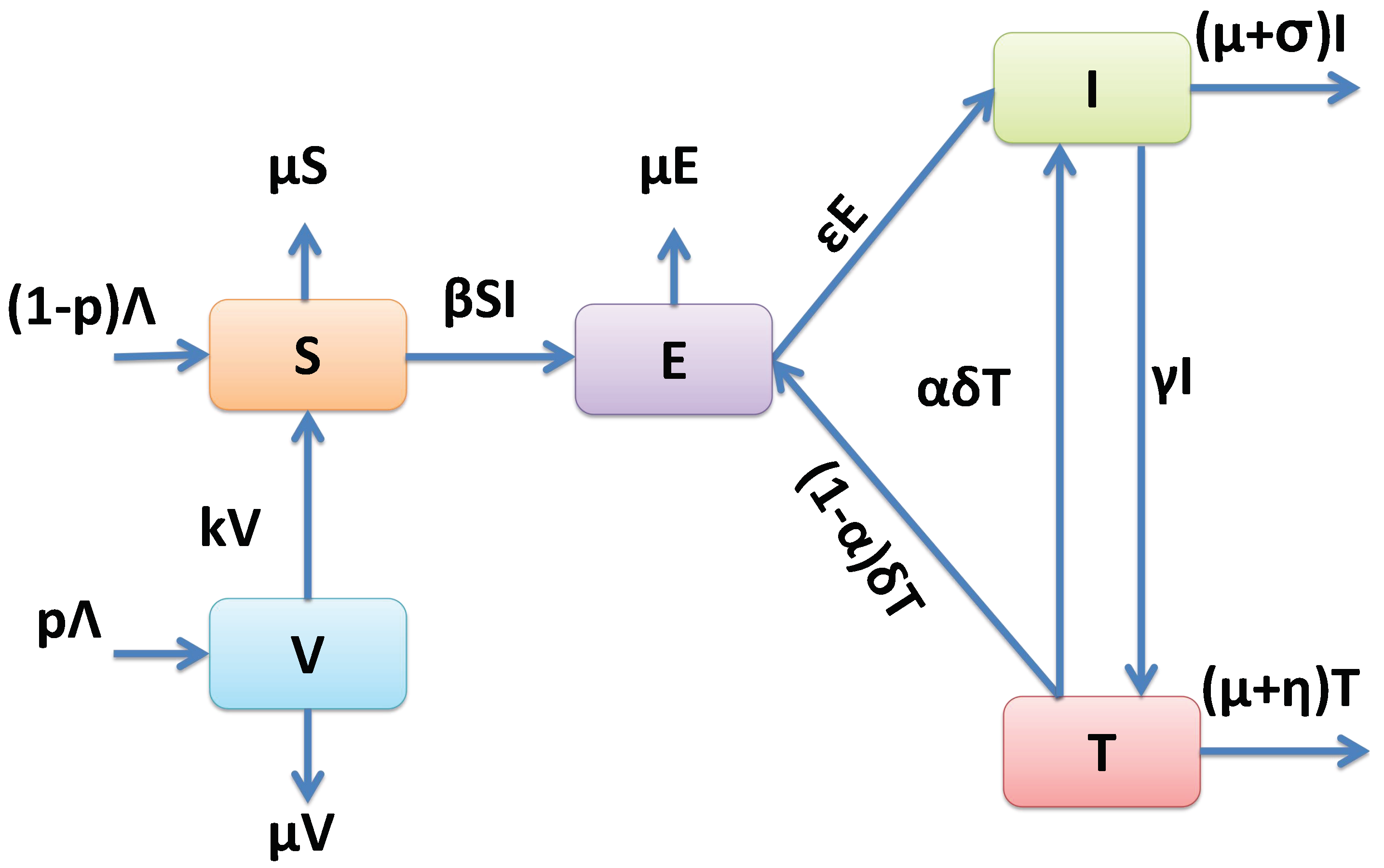
2.1. Model Formulation
2.2. Model Analysis
2.2.1. Invariance of the Feasible Region
- Thus, for , we obtain for all .
2.2.2. Equilibrium Points and Their Stability
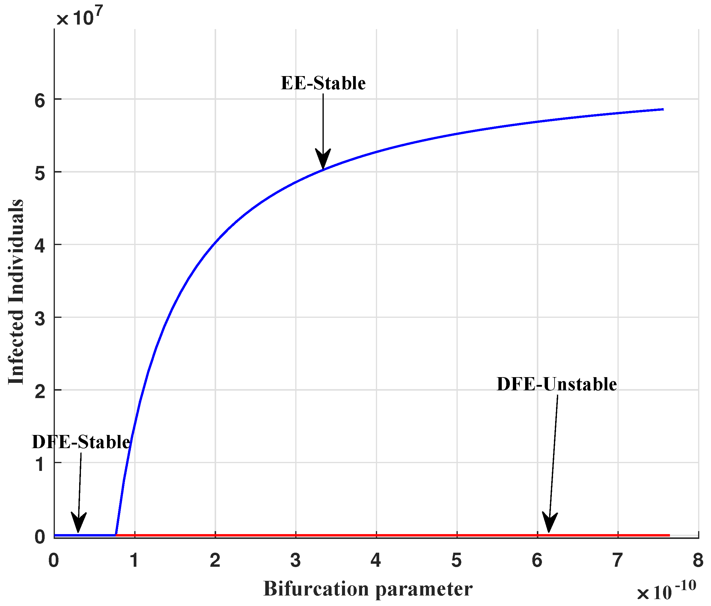
- One gets two equilibrium points:
- The disease-free equilibrium point “DFE”and the endemic equilibrium point “EE”
2.2.3. The Basic Reproduction Number
2.2.4. Local Stability Analysis of DFE
2.2.5. Global Stability Analysis of DFE
2.2.6. Local Stability Analysis of EE
2.2.7. Global Stability Analysis of EE
2.2.8. Transcritical Bifurcation Analysis
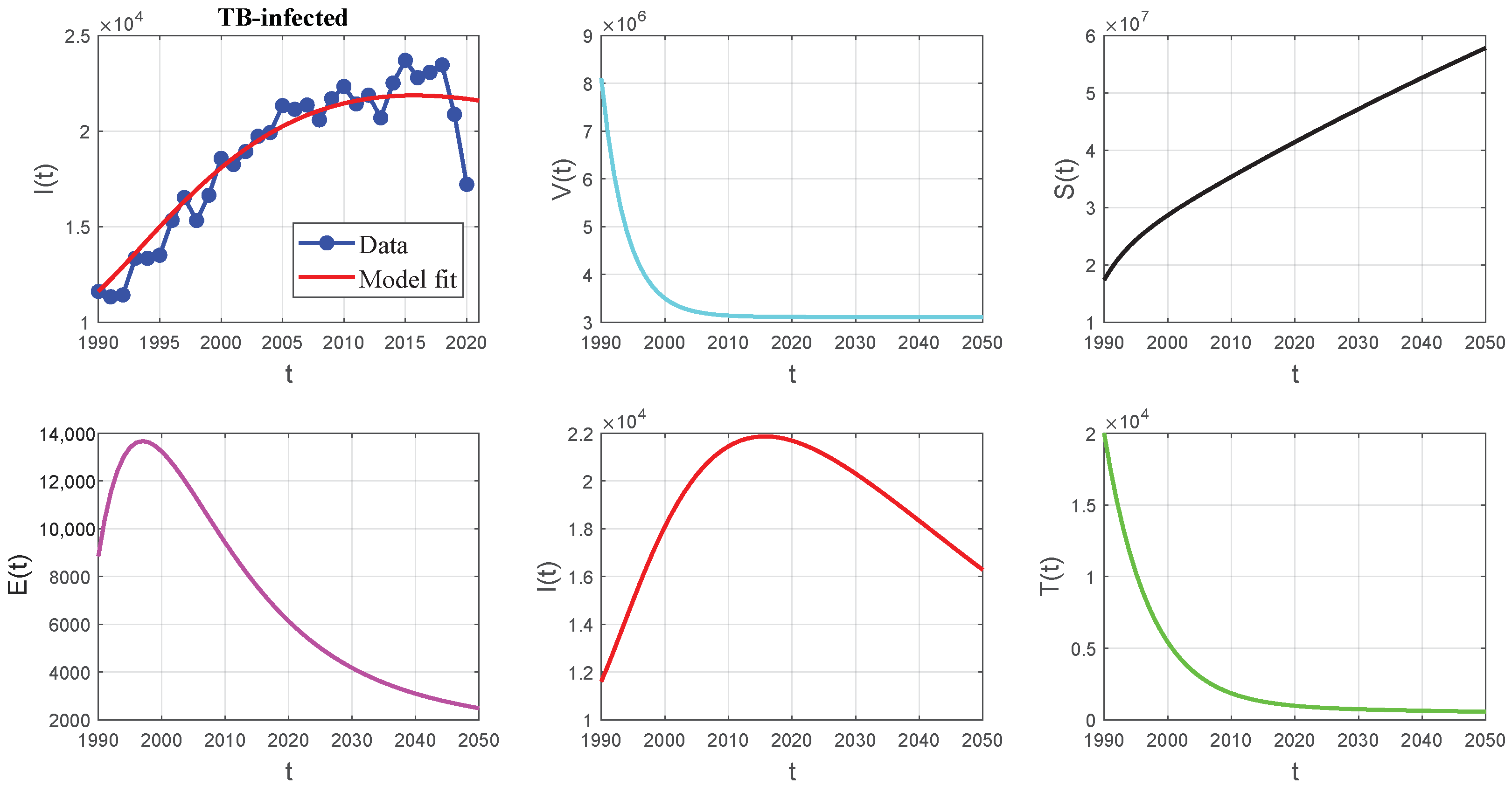
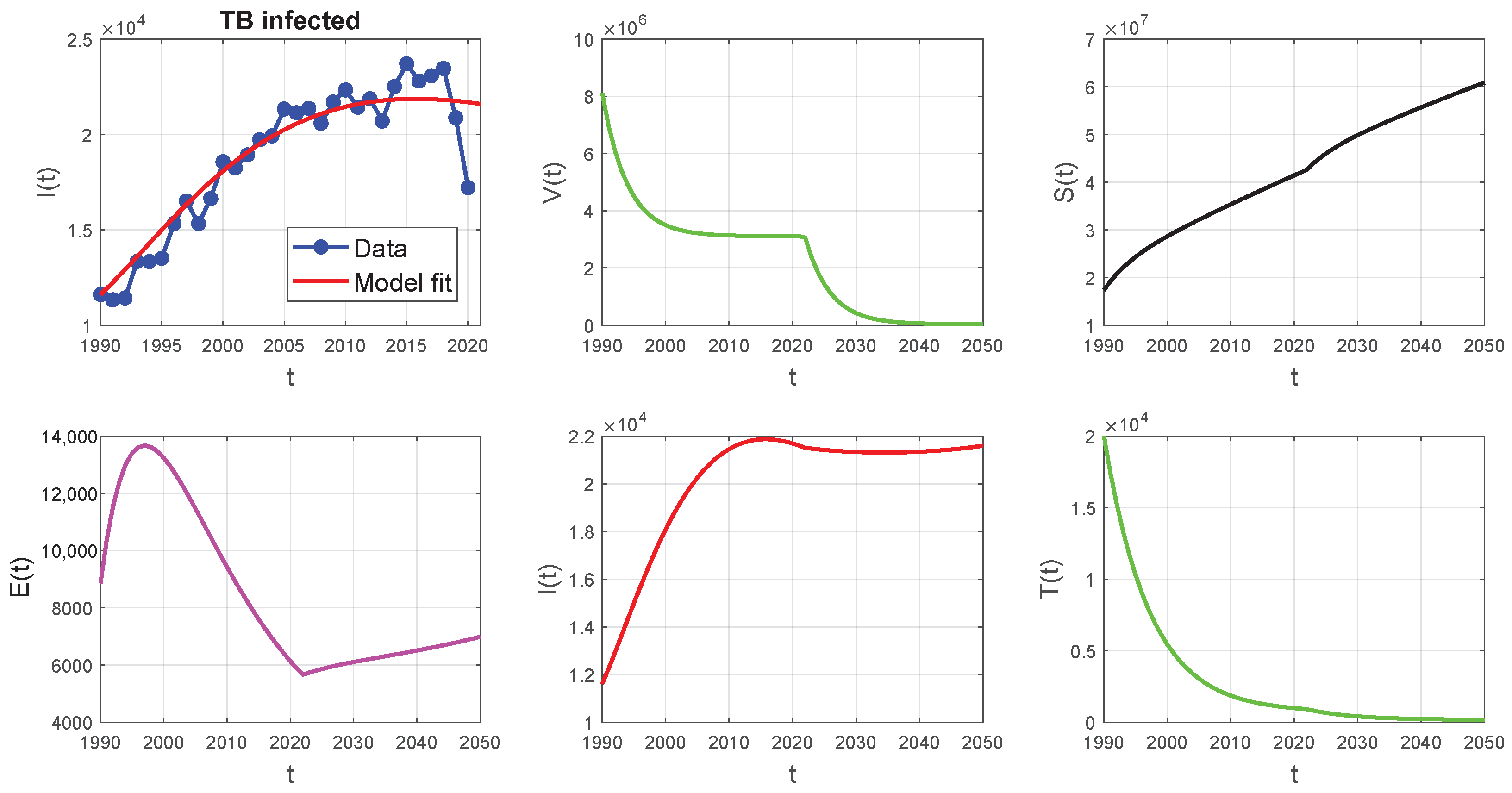
3. Parameters Estimation and Numerical Simulation
3.1. Parameters Estimation

| Parameters | Description | Algeria’s Parameters | References |
|---|---|---|---|
| Initial number of vaccinated | 8,109,389 | Assumed | |
| Initial number of susceptible | 17,368,226 | Calculated | |
| Initial number of exposed | 8852 | Assumed | |
| Initial number of infected | 11,607 | [1] | |
| Initial number of treated | 20,000 | Assumed | |
| Recruitment rate | 811,085 | [18] | |
| Natural death rate | 0.00498 | [18] | |
| k | Rate of moving from V to S | 0.25 | [19] |
| Transmission rate | Fitted | ||
| Treatment rate | 0.0043 | Fitted | |
| Progression rate | 0.0656 | Fitted | |
| Treatment failure rate | 0.1095 | [21] | |
| Rate at which the treated | 0.1325 | Fitted | |
| population leaves the class T | |||
| Disease death rate in I | 0.0136 | Fitted | |
| Disease death rate in T | Fitted | ||
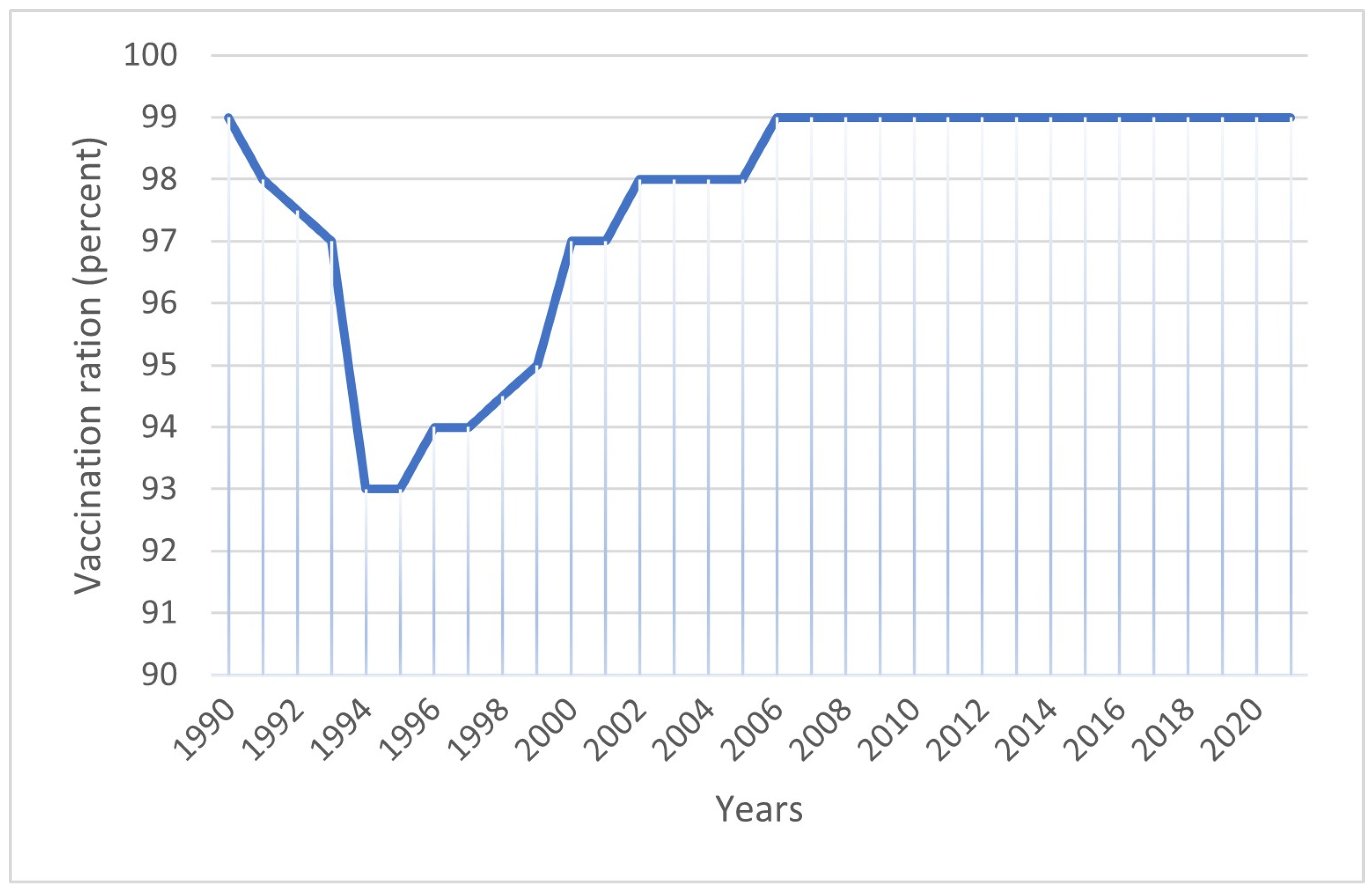
| p | Vaccination rate | 0.977 | [19] |
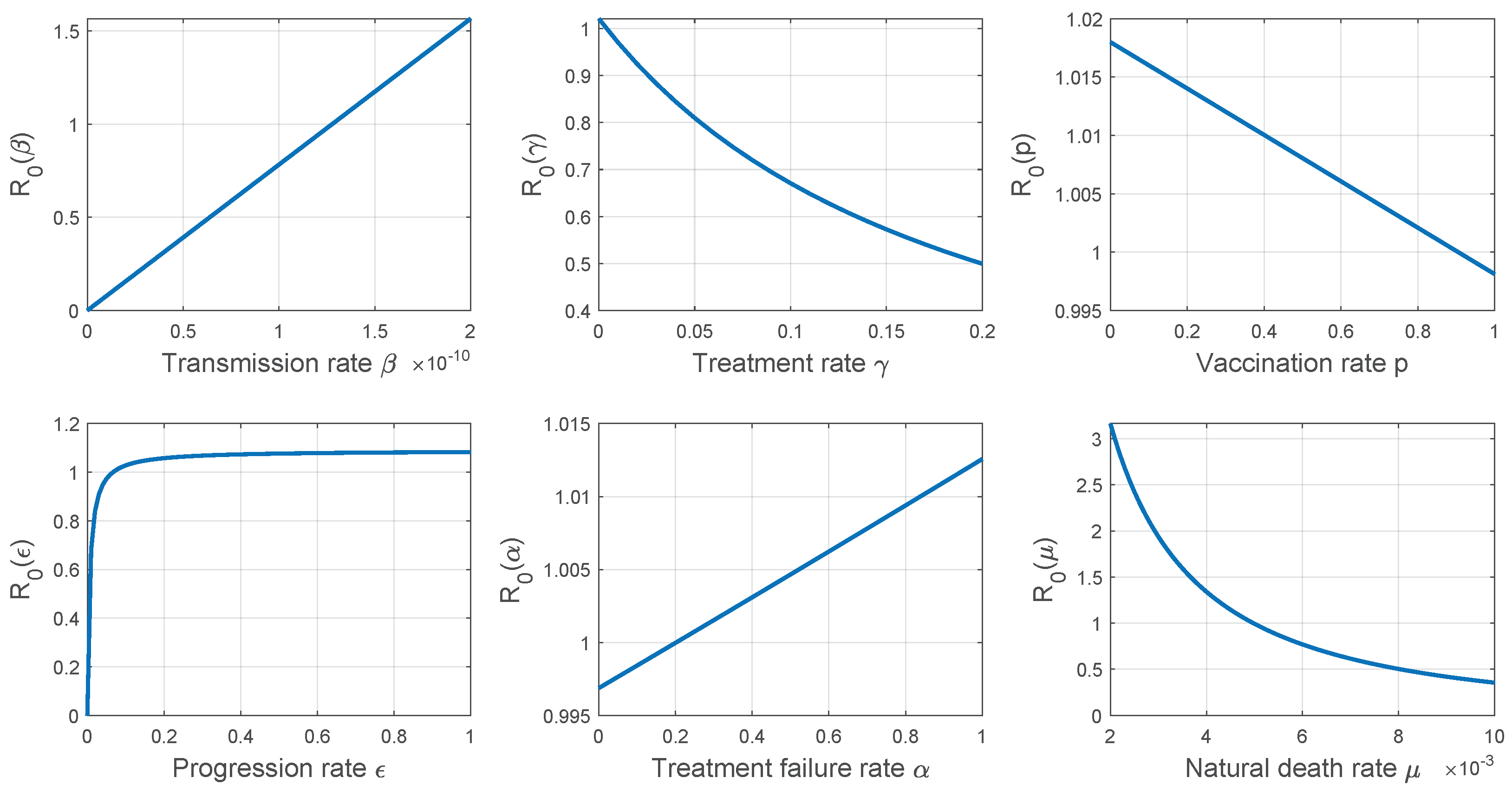
3.2. Sensitivity Analysis
4. Results and Discussion
- Enhancing the precision and quality of TB diagnosis to facilitate appropriate actions towards affected individuals.
- Imposing isolation measures on infected individuals and monitoring their families medically to minimize contact with contagious patients.
- Sustaining a high rate of vaccination for children to provide immunity.
- Increasing the treatment rate by training specialized doctors, acquiring the most potent medicines, and establishing dedicated facilities to combat this disease.
5. Conclusions
Author Contributions
Funding
Data Availability Statement
Conflicts of Interest
Appendix A. The Basic Reproduction Number
Appendix B. (LaSalle’s Invariance Principle)
- Consider the autonomous systemwhere f is of class The LaSalle’s invariance principle [23] is stated in the following theorem.
References
- WHO. Global Tuberculosis Report; World Health Organization: Geneva, Switzerland, 2023; Available online: https://extranet.who.int/tme/generateCSV.asp?ds=notifications (accessed on 1 January 2023).
- Bernoulli, D. Essai d’une Nouvelle Analyse de la Mortalité Causée par la Petite Vérole, et des Avantages de l’inoculation Pour la Prévenir. Histoire de l’Acad. Roy. Sci. (Paris) avec Mem. 1760, pp. 1–45. Available online: https://gallica.bnf.fr/ark:/12148/bpt6k3558n/f223.item.r=daniel%20bernoulli (accessed on 1 January 2023).
- Ross, R. The Prevention of Malaria. Nature 1910, 85, 263–264. [Google Scholar] [CrossRef]
- Hamer, W.H. The Milroy Lectures on Epidemic Diseases in England: The Evidence of Variability and of Persistency of Type; The Bedford Press: London, UK, 1906; pp. 733–739. [Google Scholar]
- Martini, E. Berechnungen und Beobachtungen zur Epidemiologie und Bekampfung der Malaria; W. Gente: Hamburg, Germany, 1921. [Google Scholar]
- Lotka, A.J. Elements of Physical Biology; Williams and Wilkens: Philadelphia, PA, USA, 1925. [Google Scholar]
- Yang, Y.; Tang, S.; Ren, X.; Zhao, H.; Guo, C. Global stability and optimal control for a tuberculosis model with vaccination and treatment. Discret. Contin. Dyn. Syst. Ser. B 2016, 21, 1009–1022. [Google Scholar] [CrossRef] [Green Version]
- Kermack, W.O.; McKendrick, A.G. A contribution to the mathematical theory of epidemics. Proc. R. Soc. Lond. Ser. A Contain. Pap. Math. Phys. Character 1927, 115, 700–721. [Google Scholar]
- Waaler, H.; Geser, A.; Andersen, S. The use of mathematical models in the study of the epidemiology of tuberculosis. Am. J. Public Health Nation’s Health 1962, 52, 1002–1013. [Google Scholar] [CrossRef] [PubMed]
- Ullah, S.; Khan, M.A.; Farooq, M.; Gul, T. Modeling and analysis of Tuberculosis (TB) in Khyber Pakhtunkhwa, Pakistan. Math. Comput. Simul. 2019, 165, 182–184. [Google Scholar] [CrossRef]
- Abdelouahab, M.S.; Arama, A.; Lozi, R. Bifurcation analysis of a model of tuberculosis epidemic with treatment of wider population suggesting a possible role in the seasonality of this disease. Chaos Interdiscip. J. Nonlinear Sci. 2021, 31, 123125. [Google Scholar] [CrossRef] [PubMed]
- Andersen, P.; Doherty, T.M. The success and failure of BCG-implications for novel tuberculosis vaccine. Nature 2005, 3, 656–662. [Google Scholar] [CrossRef] [PubMed]
- Ucakan, Y.; Gulen, S.; Koklu, K. Analysing of Tuberculosis in Turkey through SIR, SEIR and BSEIR Mathematical Models. Math. Comput. Model. Dyn. Syst. 2021, 27, 179–202. [Google Scholar] [CrossRef]
- Egonmwan, A.O.; Okuonghae, D. Mathematical analysis of a tuberculosis model with imperfect vaccine. Int. J. Biomath. 2019, 12, 1950073. [Google Scholar] [CrossRef]
- Revelle, C.S.; Lynn, W.R.; Feldmann, F. Mathematical models for the economic allocation of tuberculosis control activities in developing nations. Am. Rev. Respir. Dis. 1967, 96, 893–909. [Google Scholar]
- Diekmann, O.; Heesterbeek, J.A.P.; Metz, J.A. On the definition and the computation of the basic reproduction ratio R0 in models for infectious diseases in heterogeneous populations. J. Math. Biol. 1990, 28, 365–382. [Google Scholar] [CrossRef] [Green Version]
- Wang, Y.; Cao, J. Global stability of general cholera models with nonlinear incidence and removal rates. J. Frankl. Inst. 2015, 352, 2464–2485. [Google Scholar] [CrossRef]
- Population Growth in Algeria. Available online: https://www.donneesmondiales.com/afrique/algerie/croissance-population.php (accessed on 10 January 2022).
- Trading Economics. Immunization, BCG (% of One-Year-Old Children) Algeria. Available online: https://www.tradingeconomics.com/algeria/immunization-bcg-percent-of-one-year-old-children-wb-data.html/ (accessed on 20 January 2022).
- Katelaris, A.L.; Jackson, C.; Southern, J.; Gupta, R.K.; Drobniewski, F.; Lalvani, A.; Lipman, M.; Mangtani, P.; Abubakar, I. Effectiveness of BCG Vaccination Against Mycobacterium tuberculosis Infection in Adults: A Cross-sectional Analysis of a UK-Based Cohort. J. Infect. Dis. 2020, 221, 146–155. [Google Scholar] [CrossRef]
- The World Bank Group. Tuberculosis Treatment Success Rate (% of New Cases)—Algeria. Available online: https://data.worldbank.org/indicator/SH.TBS.CURE.ZS?locations=DZ (accessed on 5 January 2022).
- Van den Driessche, P.; Watmough, J. Reproduction numbers and sub-threshold endemic equilibria for compartmental models of disease transmission. Math. Biosci. 2002, 180, 29–48. [Google Scholar] [CrossRef]
- LaSalle, J.P. Some extensions of Liapunov’s second method. IRE Trans. Circuit Theory 1960, 7, 520–527. [Google Scholar] [CrossRef] [Green Version]


| Variable | Description |
|---|---|
| The vaccinated population at time t. | |
| The susceptible population which is able to be infected at any time t. | |
| The exposed population which is not yet infectious. | |
| The infected population at time t. | |
| The treated population at time t. |
| Model Parameter | Description | Unit |
|---|---|---|
| Recruitment rate | ||
| Natural death rate | ||
| k | Rate of moving from V to S | |
| Transmission rate | ||
| Treatment rate | ||
| Progression rate | ||
| Treatment failure rate | ||
| Rate at which the treated population leave the class T | ||
| Disease death rate in I | ||
| Disease death rate in T | ||
| p | Vaccination rate |
| Year | Reported Data | Numerical Value | Year | Reported Data | Numerical Value |
|---|---|---|---|---|---|
| 1990 | 11,607 | 11,607 | 2006 | 21,143 | 20,613 |
| 1991 | 11,332 | 12,162 | 2007 | 21,369 | 20,884 |
| 1992 | 11,428 | 12,793 | 2008 | 20,588 | 21,116 |
| 1993 | 13,345 | 13,471 | 2009 | 21,701 | 21,313 |
| 1994 | 13,345 | 14,137 | 2010 | 22,336 | 21,474 |
| 1995 | 13,507 | 14,880 | 2011 | 21,429 | 21,604 |
| 1996 | 15,329 | 15,578 | 2012 | 21,880 | 21,705 |
| 1997 | 16,522 | 16,255 | 2013 | 20,701 | 21,778 |
| 1998 | 15,324 | 16,255 | 2014 | 22,517 | 21,825 |
| 1999 | 16,647 | 17,517 | 2015 | 23,705 | 21,850 |
| 2000 | 18,572 | 18,090 | 2016 | 22,801 | 21,854 |
| 2001 | 18,250 | 18,621 | 2017 | 23,077 | 21,838 |
| 2002 | 18,934 | 19,108 | 2018 | 23,465 | 21,805 |
| 2003 | 19,730 | 19,550 | 2019 | 20,879 | 21,757 |
| 2004 | 19,929 | 19,947 | 2020 | 17,212 | 21,694 |
| 2005 | 21,336 | 20,301 | 2021 | - | 21,619 |
| Parameter | Sensitivity Index |
|---|---|
| k | +0.0012 |
| p |
Disclaimer/Publisher’s Note: The statements, opinions and data contained in all publications are solely those of the individual author(s) and contributor(s) and not of MDPI and/or the editor(s). MDPI and/or the editor(s) disclaim responsibility for any injury to people or property resulting from any ideas, methods, instructions or products referred to in the content. |
© 2023 by the authors. Licensee MDPI, Basel, Switzerland. This article is an open access article distributed under the terms and conditions of the Creative Commons Attribution (CC BY) license (https://creativecommons.org/licenses/by/4.0/).
Share and Cite
Chennaf, B.; Abdelouahab, M.S.; Lozi, R. Analysis of the Dynamics of Tuberculosis in Algeria Using a Compartmental VSEIT Model with Evaluation of the Vaccination and Treatment Effects. Computation 2023, 11, 146. https://doi.org/10.3390/computation11070146
Chennaf B, Abdelouahab MS, Lozi R. Analysis of the Dynamics of Tuberculosis in Algeria Using a Compartmental VSEIT Model with Evaluation of the Vaccination and Treatment Effects. Computation. 2023; 11(7):146. https://doi.org/10.3390/computation11070146
Chicago/Turabian StyleChennaf, Bouchra, Mohammed Salah Abdelouahab, and René Lozi. 2023. "Analysis of the Dynamics of Tuberculosis in Algeria Using a Compartmental VSEIT Model with Evaluation of the Vaccination and Treatment Effects" Computation 11, no. 7: 146. https://doi.org/10.3390/computation11070146