
Extended Online DMD and Weighted Modifications for Streaming Data Analysis


Faculty of Mathematics and Informatics, Shumen University, 9700 Shumen, Bulgaria
Computation 2023, 11(6), 114; https://doi.org/10.3390/computation11060114
Submission received: 5 May 2023
/
Revised: 1 June 2023
/
Accepted: 6 June 2023
/
Published: 9 June 2023
(This article belongs to the Special Issue Mathematical Modeling and Study of Nonlinear Dynamic Processes)
Abstract
:We present novel methods for computing the online dynamic mode decomposition (online DMD) for streaming datasets. We propose a framework that allows incremental updates to the DMD operator as data become available. Due to its ability to work on datasets with lower ranks, the proposed method is more advantageous than existing ones. A noteworthy feature of the method is that it is entirely data-driven and does not require knowledge of any underlying governing equations. Additionally, we present a modified version of our proposed approach that utilizes a weighted alternative to online DMD. The suggested techniques are demonstrated using several numerical examples.
1. Introduction
Dynamic mode decomposition (DMD) has become increasingly popular in studying complex dynamical systems. Since it was introduced for the first time by Schmid [1], it has been successfully applied to a wide range of problems, such as video processing [2], epidemiology [3], neuroscience [4], financial trading [5,6,7], robotics [8], cavity flows [9,10], and various jets [11,12]. For a review of the DMD literature, we refer the reader to [13,14,15,16,17]. For some recent modifications of DMD for non-uniformly sampled data, the higher-order DMD method, parallel implementations of DMD, and some derivative DMD techniques, we recommend [18,19,20,21,22,23,24,25,26,27,28,29].
In this work, we are interested in a recently developed modification of the DMD method called online dynamic mode decomposition (online DMD) [30] (see also [31,32]). We introduce an alternative online DMD method that is applicable for both overconstrained and underconstrained datasets.
The outline of this paper is as follows. In the rest of this section, we give a brief summary of the online DMD and alternative online DMD methods. In Section 2, we introduce and discuss the new approach of the online DMD method. In Section 3, we present examples demonstrating the new algorithm. The conclusion is in Section 4.
1.1. Online Dynamic Mode Decomposition (Online DMD)
In this subsection, the Algorithm 1 of so-called online dynamic mode decomposition (online DMD) is introduced, following the description in [30].
It requires a dataset of snapshot pairs
spaced a fixed time interval apart. Then, the snapshots are stacked into the following pair of matrices:
The following assumptions are made:
- The number of snapshots k is large compared with the state dimension n (i.e., we consider the overconstrained case of the dataset, where ).
- The matrix has full row rank (i.e., ).
The objective of the online DMD method is to provide an alternative way of computing the DMD operator such that it can be updated incrementally as new snapshots become available. The algorithm of online DMD proceeds as follows [30]:
| Algorithm 1 Online DMD Method [30] |
|
1.2. Alternative Online DMD
A novel approach was introduced in [33] to overcome the main shortcomings of online DMD. The new scheme is designed to work with low-rank data, and the condition has been relaxed.
Consider a time series of data with snapshots organized into the following two data matrices:
Then, the truncated SVD is performed, where , , , and is the truncation value. The low-dimensional DMD operator is calculated using the formula .
A single iteration of the modified algorithm can be summarized as follows [33].
In this study, we aim to improve the alternative online DMD method (Algorithm 2) from a computational perspective. The next section shows how matrix can be expressed by using a diagonal-plus-rank-one matrix (DPR1 matrix) instead of matrix (or ) in Step 1 of Algorithm 2. As a result, the eigendecomposition of a DPR1 matrix can be used instead of the SVD of a matrix of the same dimension.
| Algorithm 2 Alternative Online DMD Method |
| Input: Matrices , scalar , last 3 snapshots . Compute and proceed: If :
Else If :
|
2. Improved Online DMD
Through analogy with the online DMD, let us consider the k snapshot pairs for as in Equation (1). We form matrices
which both have dimensions of . Then, the truncated SVD
is performed, where , , and . The truncation value r is such that , and it is a predefined value. From the pseudoinverse , we express the DMD operator
The projected DMD operator has the form
which is of dimension . We can perform the leading eigendecomposition of by using the eigendecomposition of .
Suppose now that we have already computed (or ) for a given dataset. Whenever a new pair of snapshots becomes available , we would like to compute matrix more efficiently than how it is usually carried out (Equation (6)).
Let us denote the augmented matrices
Suppose that the singular value decomposition of has the form
From Equation (8), we express as
Then, the updated DMD operator has the form
By substituting Equation (7) into the last expression, we obtain
Using the SVD of , we obtain
By applying Equation (5), the last expression yields
Equation (13) gives a rule for computing given , and the new snapshot pair .
In what follows, we will show that matrices and can be expressed from matrices and . For this purpose, we consider the covariance matrix
which has the following presentation:
by using Equation (7) and the SVD of . It is well known that the leading left singular vectors and singular values of can be computed by the eigendecomposition of . We will consider two scenarios in order to obtain an alternative representation of the SVD of , depending on whether :
(1) If , then the expression
is valid, and the covariance matrix can be presented as
where we define
as a diagonal-plus-rank-one (DPR1) matrix of a dimension . In this case, the eigendecomposition of can be reduced to that of a DPR1 matrix plus two matrix multiplications. Assume that the eigendecomposition of the matrix has the form
where is unitary and is diagonal. Then, for the left singular vectors and singular values of , we obtain
Now, from Equation (13), we can express the matrix as
(2) If , then let us define
and
We denote the matrix
It is straightforward that
By applying the last two expressions in Equation (15), the formula for becomes
which is an hermitian matrix. From Equation (24) and the definition of follows the identity
where is a zero vector and is the identity matrix.
By substituting Equation (26) into Equation (25), we obtain
where
is a diagonal-plus-rank-one (DPR1) matrix of the dimensions . Assume that the eigendecomposition of is
where is unitary and is diagonal. Then, for the left singular vectors of (or the eigenvectors of ) and singular values of , we obtain
Furthermore, we can compute the reduced-order approximation of :
which is an matrix. An equivalent representation of using the expression in Equation (26) and the definition of is
where the following expression holds:
In the particular case of for , from the orthogonality of and , it follows that
Therefore, we have
where is the last row of matrix . From the SVD of , it follows that
which yields the last column of :
The next paragraph summarizes the obtained results as an improved variant of Algorithm 2.
Algorithm for Improved Alternative Online DMD
Let us consider a time series of data with snapshots organized into the following two data matrices:
Then, we compute the truncated SVD of as in Equation (4), where is the truncation value, and compute the matrix as in Equation (6).
For each new data point , the first task is to determine whether the basis contained in should be expanded. To accomplish this, the residual is computed, and if is greater than some pre-specified tolerance , then we expand by appending .
A single iteration of the updated algorithm can be summarized as follows.
The main advantages of the presented algorithm over Algorithm 2 are in Step 1 and Step 2. Algorithm 3 uses a matrix with a simpler structure in Step 1 (in both parts), namely the DPR1 matrix (or , respectively). In addition, at Step 2 in Algorithm 3, spectral decomposition of a DPR1 matrix is used instead of SVD of a regular matrix.
| Algorithm 3 Improved Online DMD Method |
| Input: Matrices , scalar , last 3 snapshots . Output: Matrices . Compute and proceed: If :
Else If :
|
The main advantages of Algorithm 3 (as well as Algorithm 2) over Algorithm 1 are that it does not require full rank data matrix, and unlike Algorithm 1, Algorithm 3 (and Algorithm 2) does not require the number of snapshots to be greater than the state dimension.
In the next section, we present the framework with which Algorithm 3 (and Algorithm 2) can be modified to a weighted alternative.
3. Weighted Modifications to Online DMD
The algorithms described above are suitable for time-varying systems. They allow the DMD matrix to be updated in real time. In such cases, we may want to give more weight to recent snapshots and less weight to older snapshots. This can be achieved by using a modified cost function. As is known in the standard DMD method, for the given data matrices and in Equation (3), the DMD operator is found by minimizing the following cost function:
where denotes the Euclidean norm on the vectors and denotes the Frobenius norm on the matrices.
In cases where the system changes over time to give more weight to newer snapshots than older snapshots, we can use the modified cost function
for some constant where . In fact, for , the two formulas match, and for , errors in past snapshots are discounted.
We will show below that Algorithm 3 can easily be modified to use this weighting scheme (i.e., to minimize a cost function of the form in Equation (36) instead of the original cost function in Equation (35)). For convenience, let us denote , where , and write the cost function (2) as
Let us define the matrices based on scaled versions of the snapshots as
Then, the cost function in Equation (37) can be written as
The DMD operator , which is a unique solution that minimizes this cost function, is given by
where the truncated SVD is used. Then, the reduced-order DMD operator will have the form
On the next (th) step, we want to compute . Let us denote
and
By analogy with Section 2, we can repeat the expressions from Equation (8) to Equation (12) to obtain
for the updated DMD matrix, where and are the singular vectors and value matrices of , respectively.
In a similar way to that in Equations (14) and (15), we can extract the singular vectors and singular values of through the eigendecomposition of
Matrix differs from in Equation (15) only by a factor of . Again, we will have two scenarios, depending on whether . At each step, we have to factorize one of the following two matrices:
or
where , , and . The matrices and differ only by a factor of from the corresponding matrices and in Equations (18) and (28), respectively. Then, the singular vectors and values of are given by
where and are from the eigendecomposition of or .
The reduced order DMD matrix is then given by
or
for the two considered scenarios. Observe that the updates in Equations (45) and (46) for the reduced order approximation are similar to the updates in Equations (31) and (32). The only difference is the factor of .
Therefore, the algorithm for weighted alternative online DMD follows the same steps as in Algorithm 3. The only difference is the calculation of matrices (or ) and , where Equations (42), (43) and (45), (46) are used, respectively. We have to note that the choice of the weighting factor matters. Therefore, for example, choosing will ensure that snapshots have a half-life of m samples [30]. In practice, the choice of depends on the rate of change of the dynamics. Choosing a smaller value will result in faster tracking while making the model more sensitive to noise in the data.
4. Numerical Illustrations
The new algorithm (Algorithm 3), introduced in Section 2, offers the advantage of being more cost-effective than the alternative algorithm (Algorithm 2). Considering that Algorithms 2 and 3 produce identical results, in this part, we will mainly present the results of the application of Algorithm 3 and its comparison with standard methods.
Example 1.
An illustrative example of a toy.
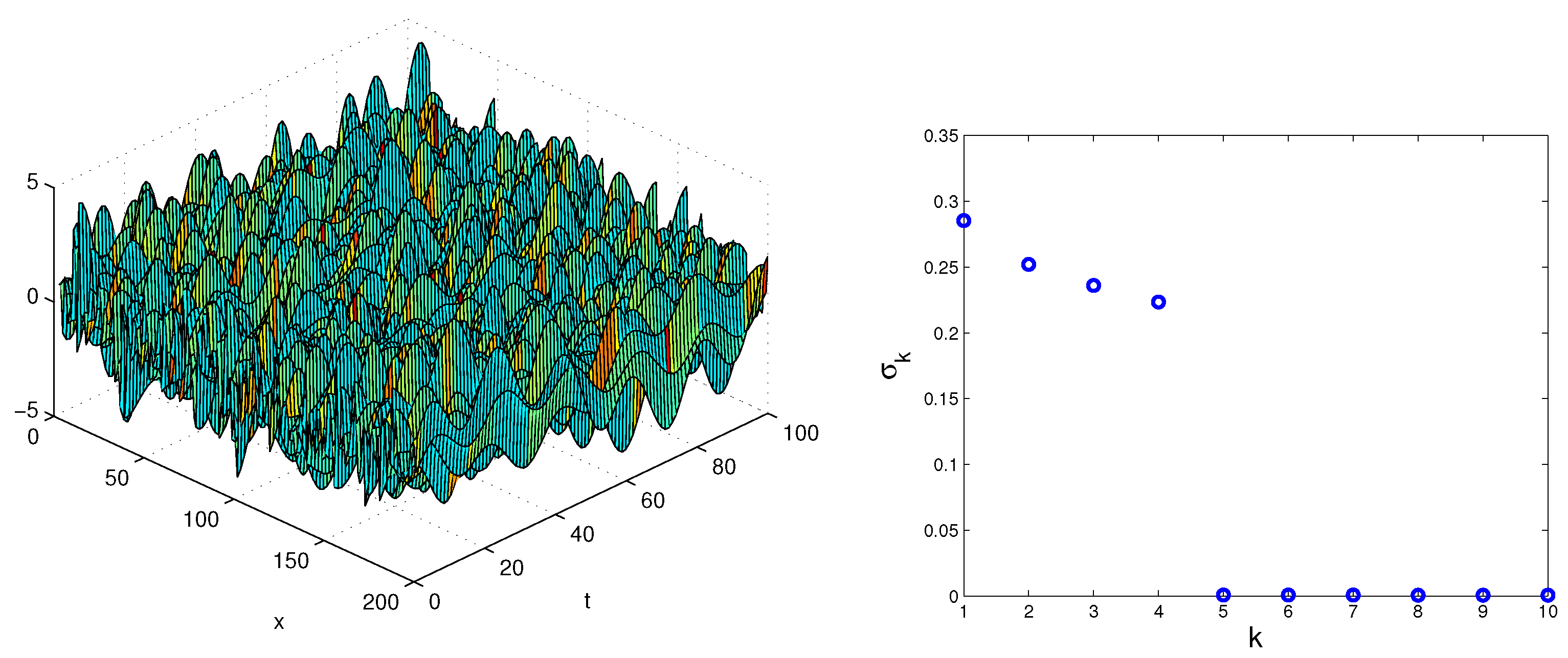
We consider a simple example of incrementally updated DMD in a toy problem. In this example, we have an arbitrary n-dimensional dynamical system with two characteristic frequencies. A total of m snapshot pairs are measured sequentially and are subject to additive zero-mean Gaussian noise with covariance:
where are random state directions, are the characteristic frequencies, is the time sampling, and is the independent identically distributed zero-mean Gaussian noise with covariance .
For the simulation, we set the parameters as follows: , , , , , and . By using the built-in function in Matlab, we defined the vectors and via the following syntax:
The 3D visualization of the dynamics is illustrated in Figure 1. The singular values of data matrix X, illustrated in Figure 1, show that the data can be adequately represented by the rank-four () approximation.
The standard online DMD method (Algorithm 1) is not applicable in this case because . Therefore, here we will compare the standard DMD method and improved online DMD method (Algorithm 3). We initialized the improved online DMD algorithm with the first three snapshots () (i.e., the initial matrices and have the form and , respectively).
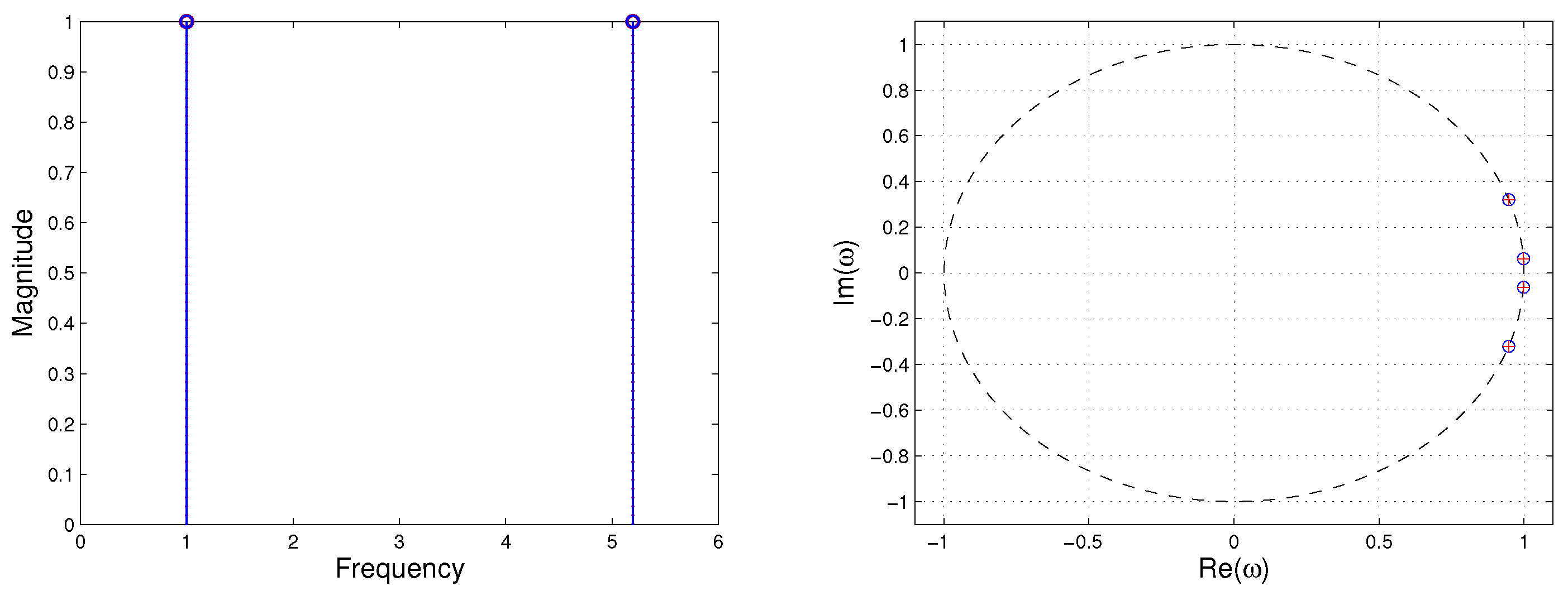
We performed both methods with rank reduction of . The two algorithms, standard DMD and Algorithm 3, were applied to different numbers of snapshots in the interval from 50 to 100. All runs of both algorithms yielded the same DMD eigenvalues shown in Figure 2.
To make quantitative comparisons among alternative online DMD and standard DMD, we computed the norm of the difference between the spatial modes extracted by the two algorithms. We computed the residual errors as follows:
for , where and denote the DMD modes computed by both algorithms. The error values for two cases at 50 and 100 snapshots are shown in Table 1.
Example 2.
Flow around a cylinder wake ().
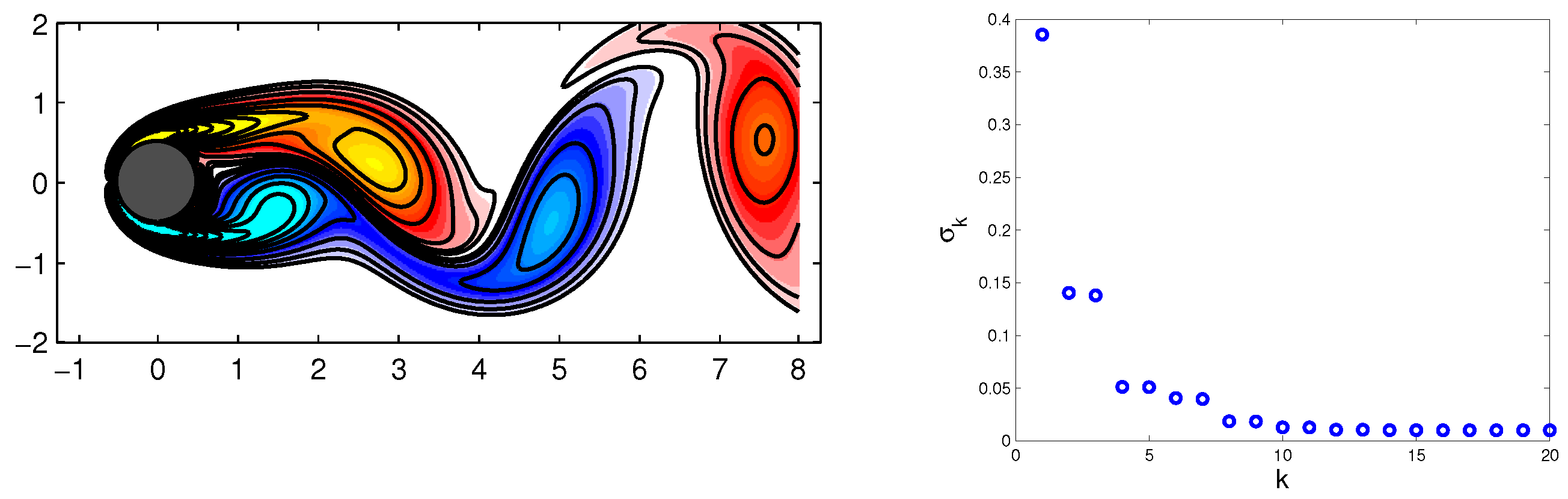
In this example, we consider a dataset representing a time series of fluid vorticity fields for the wake behind a circular cylinder at Reynolds number . The data for this example are publicly available at www.siam.org/books/ot149/flowdata (see [15]). The collected data consisted of snapshots at regular intervals in time , where , sampling five periods of vortex shedding.
Each vorticity field snapshot from the finest computational domain was reshaped into a large vector , and these vectors comprised columns of matrices X and Y, as described in Equation (34). A snapshot example of the cylinder wake data is shown in Figure 3.
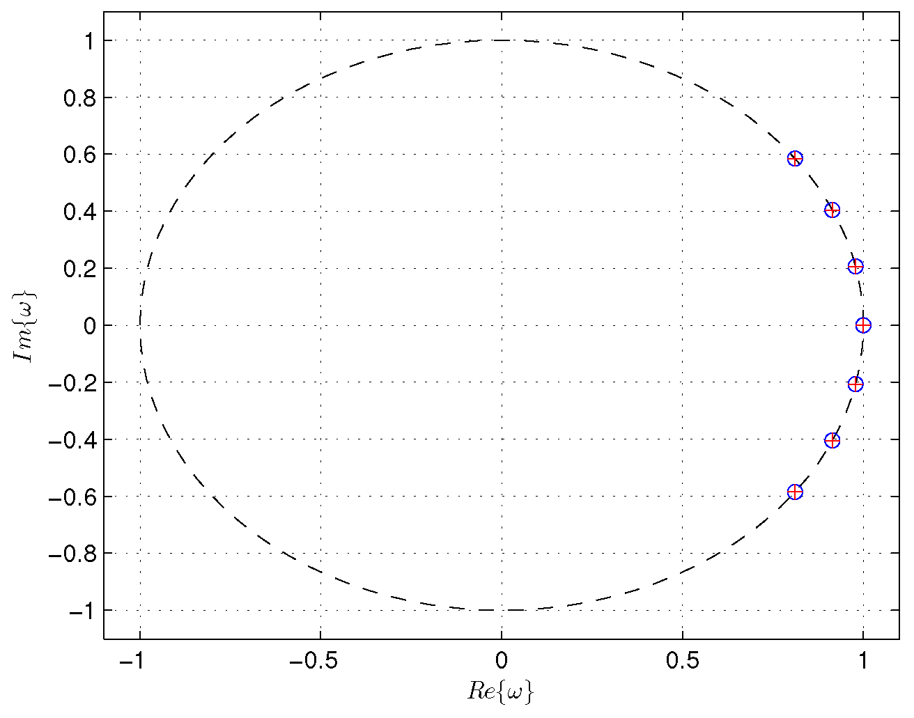
Here, we compare the standard DMD method and the improved online DMD method, since online DMD (Algorithm 1) is not applicable. In order to capture the low-dimensional dynamic, we performed rank-seven truncation. We used Algorithm 3 to obtain the DMD reconstruction of the data. The two algorithms reproduced the same DMD eigenvalues and modes. We compared the results with the standard DMD algorithm for the same rank-seven truncation. The DMD eigenvalues computed by the improved alternative online DMD and standard DMD algorithms are shown in Figure 4.
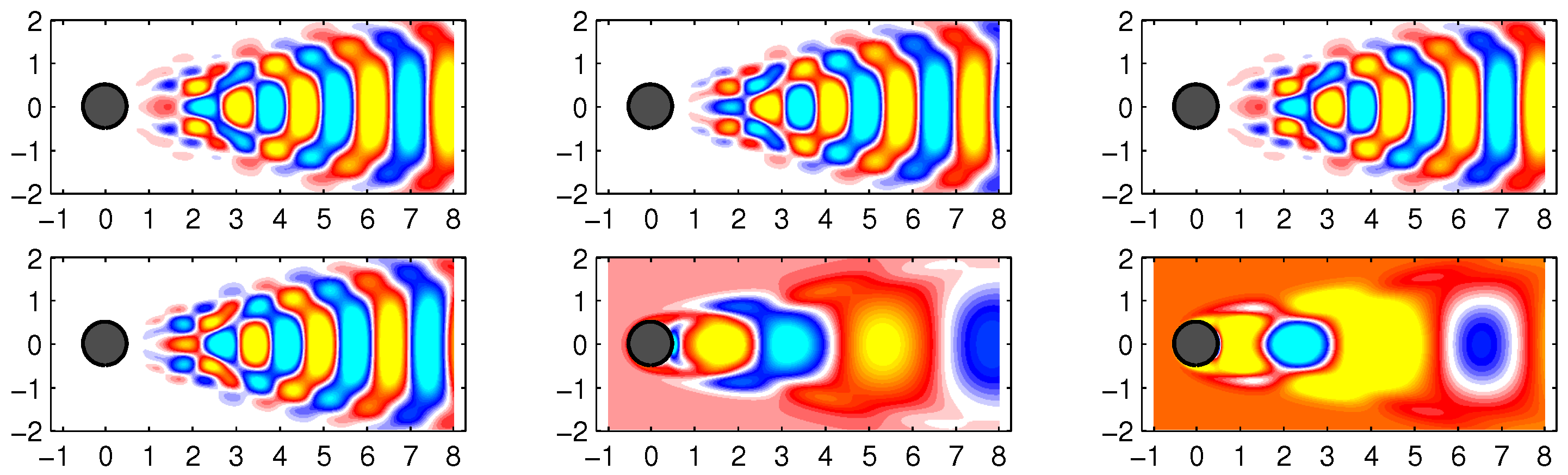
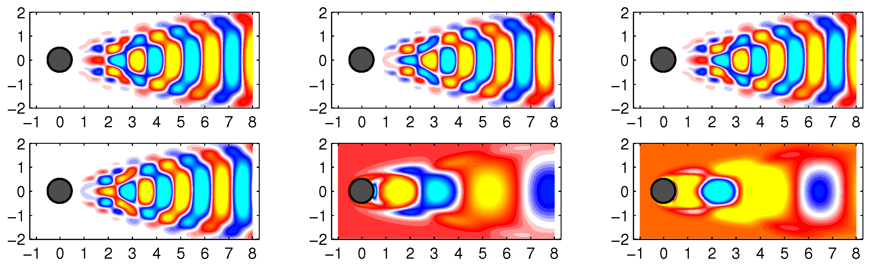
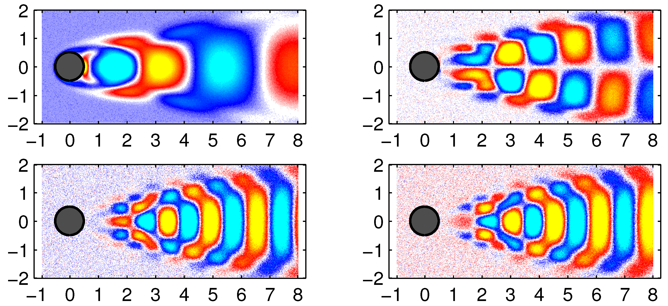
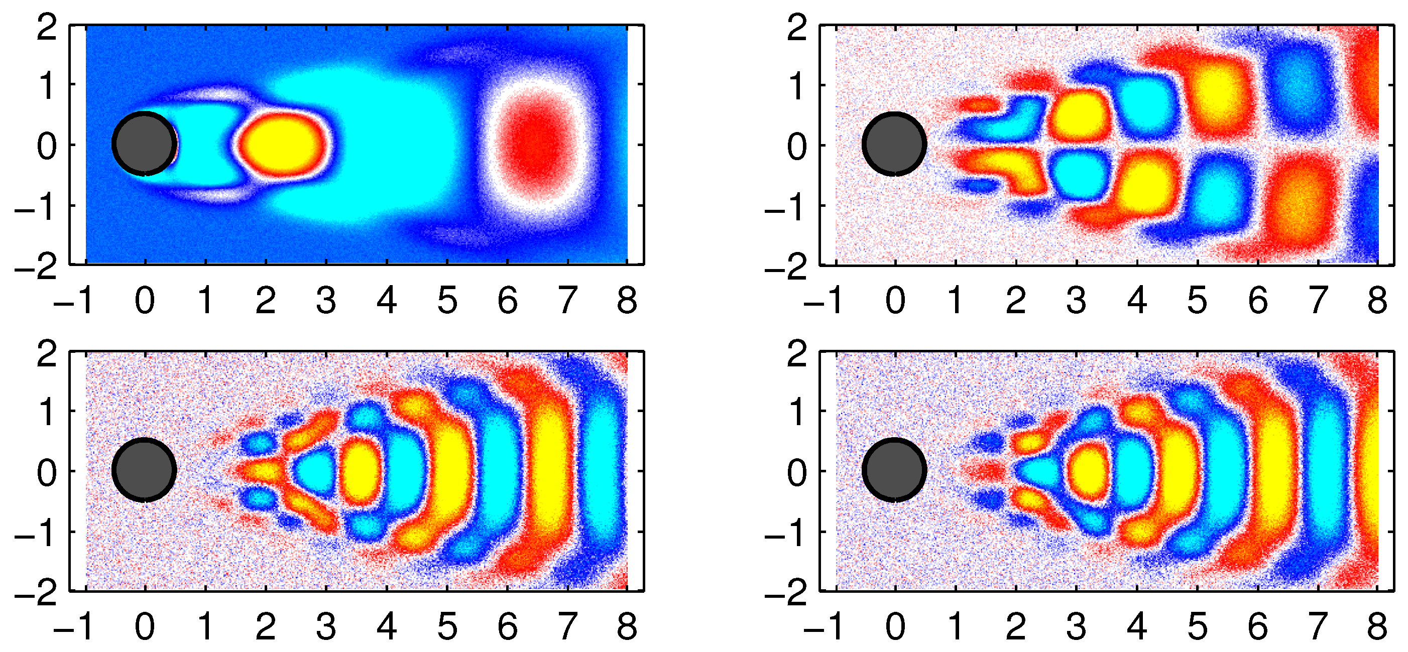
The first 6 DMD modes computed by the improved online DMD and standard DMD algorithms are shown in Figure 5 and Figure 6, respectively.
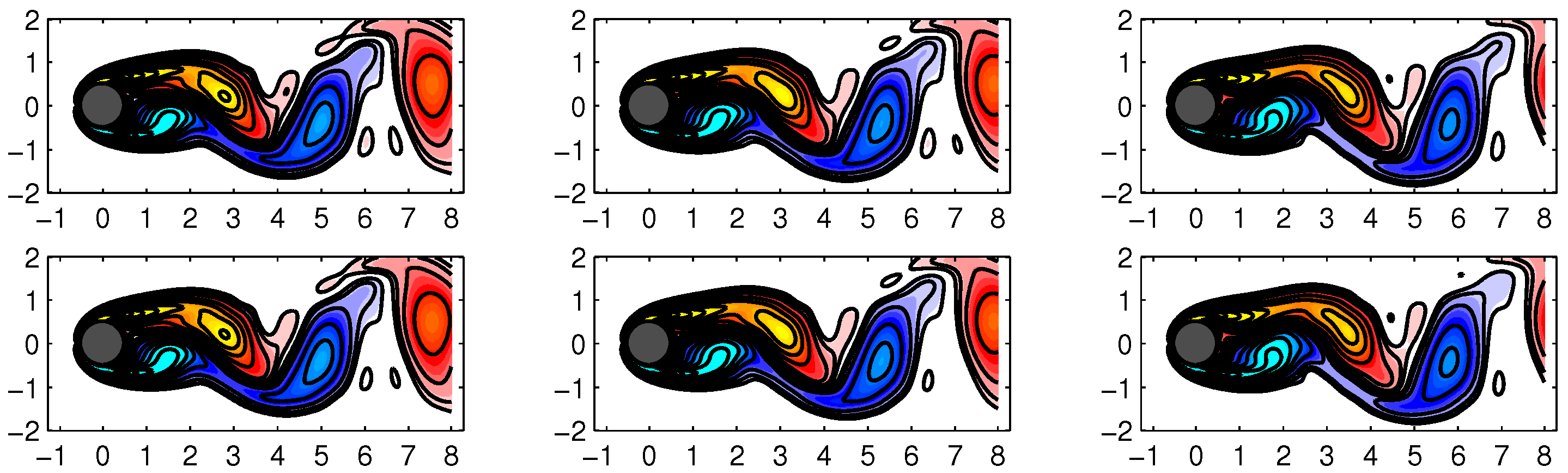
In Figure 7, some examples of data reconstruction by the standard DMD and improved online DMD methods are shown.
There was no distinction between the DMD modes and eigenvalues generated by the standard DMD algorithm (Algorithm 1) and Algorithm 3.
Example 3.
Flow around a cylinder wake with added noise.
It is well known that the DMD method’s performance depends on the cleanliness of the data collected. The noise in the collected data can affect the discovered model’s accuracy. In this example, we consider the same fluid vorticity fields for the wake behind a circular cylinder at Reynolds number , as in Example 2. Measurement noise was generated by adding Gaussian white noise to the data matrix.
As in Example 2, the data-set consisted of snapshots , where each snapshot had coordinates (i.e., the data matrix ).
The updated snapshots were generated by
where is a zero-mean Gaussian white noise process with unit standard deviation. In this example, we kept the noise variance fixed at .
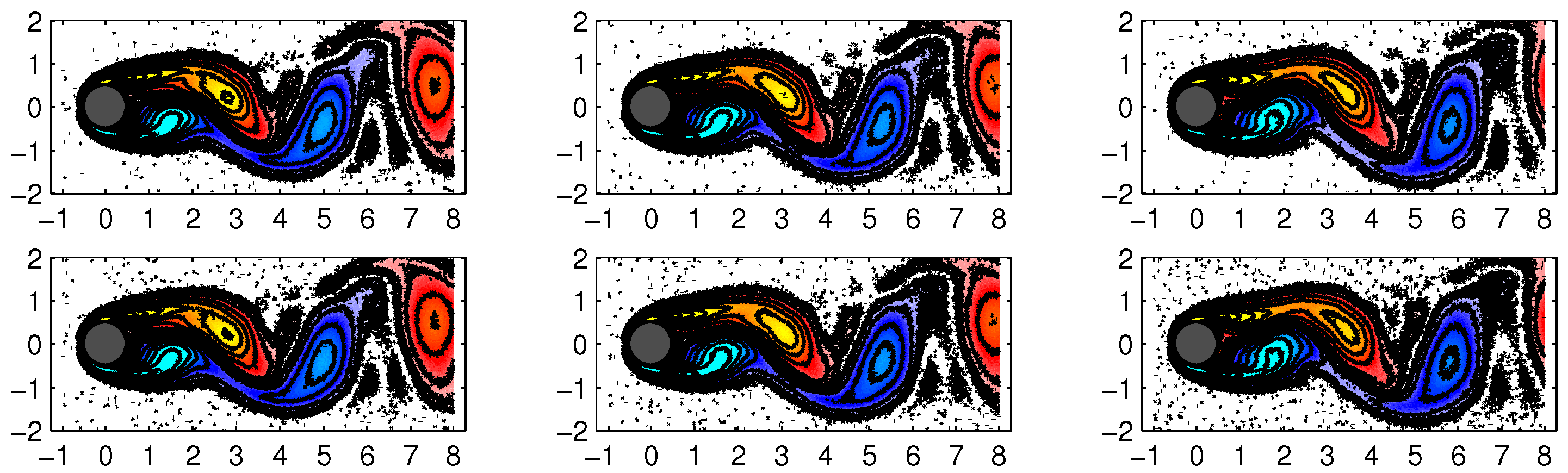
Here, we compare the standard DMD method and the improved online DMD method. As in Example 2, we performed rank-seven truncation. We used Algorithm 3 to obtain the DMD reconstruction of the data. The two algorithms reproduced the same DMD eigenvalues and modes. Figure 8 shows some examples of data reconstruction by the standard DMD and improved online DMD methods for the noisy flow data.
The first four DMD modes computed by the improved online DMD and standard DMD algorithms are shown in Figure 9 and Figure 10, respectively.
Note again that there was no distinction between the modes generated by the standard DMD algorithm and Algorithm 3. The visualizations of the DMD eigenvalues calculated by the improved alternative online DMD method and the standard DMD method were omitted as they matched those shown in Figure 4.
Example 4.
Linear time-varying system.
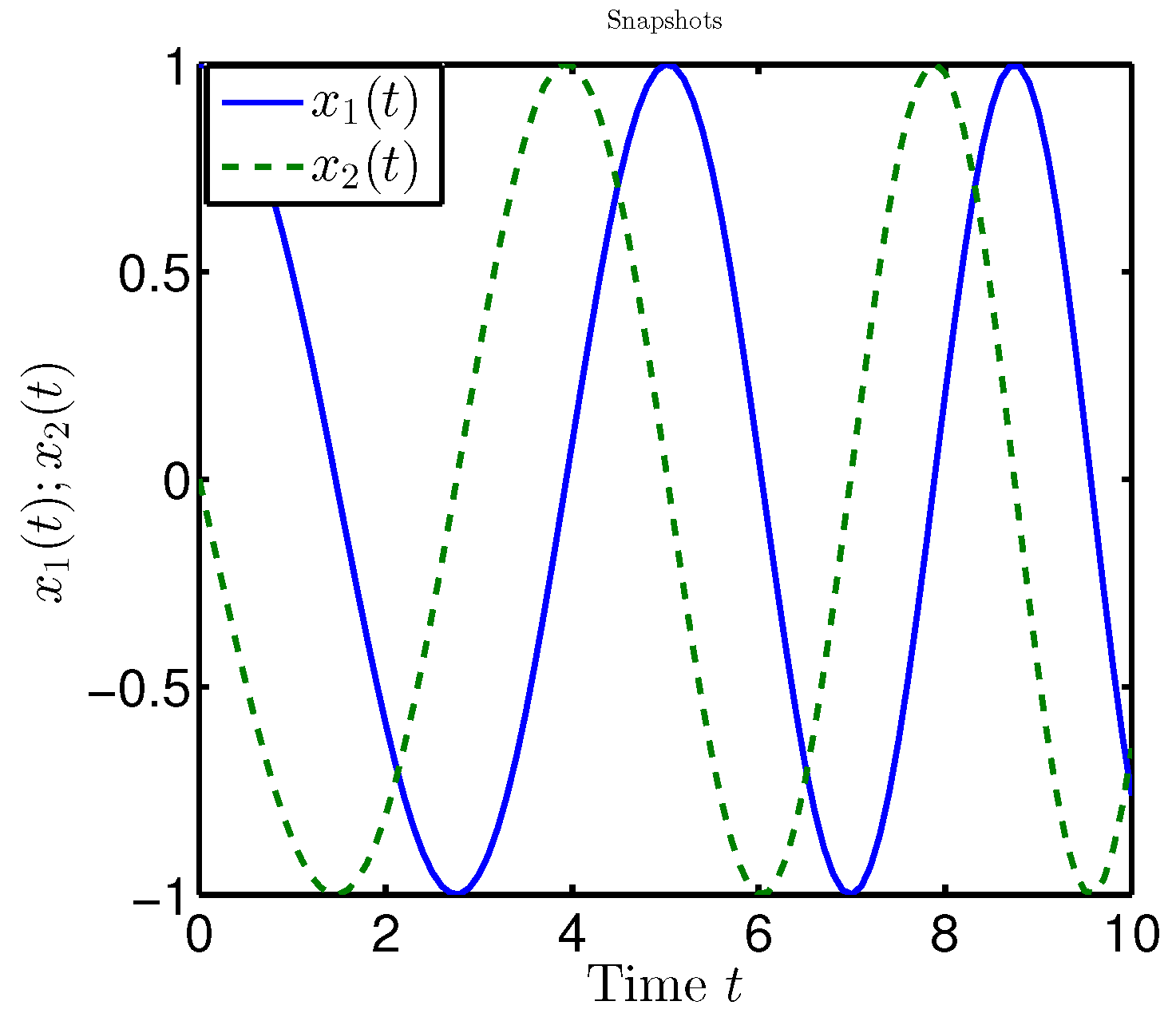
We now illustrate the improved alternative online DMD algorithm in a simple linear system that slowly varies over time:
where , and the time-varying matrix A(t) is given by
where (see [30]). The eigenvalues of are , and is constant in t. We simulated the system for from the initial condition , and the snapshots were taken with a time step of , as shown in Figure 11.
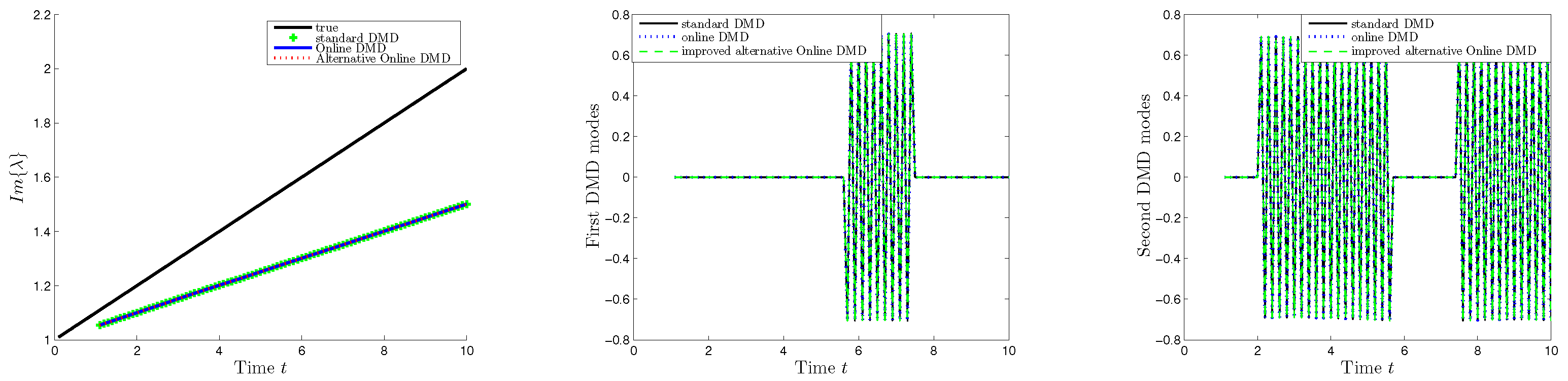
With the snapshots as input, we applied standard DMD, online DMD (Algorithm 1), and improved alternative online DMD (Algorithm 3) and compared the results. The three methods used the first snapshot pairs to initialize and start iterating from time . The discrete-time eigenvalues computed by the algorithms were converted to continuous-time DMD eigenvalues by the formula
where is the time spacing between snapshot pairs. Observe from Figure 12 that the eigenvalues computed by the alternative online DMD algorithm agreed with those identified by the standard DMD and online DMD algorithms. The true eigenvalues are also shown for comparison. The DMD modes calculated by the three algorithms were also identical, as can be seen from Figure 12.
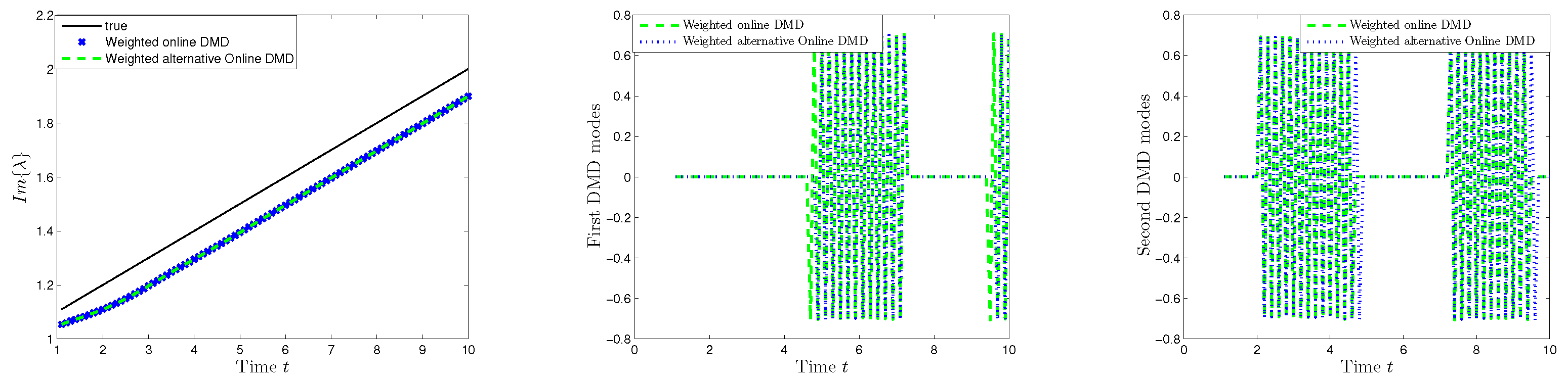
The alternative weighted online DMD algorithm was applied under the same conditions. A comparison was made between the results of the weighted variant of Algorithm 3 and the weighted online DMD algorithm introduced in [30].
As before, the results show identical DMD modes and DMD eigenvalues for both algorithms. Figure 13 shows the eigenvalues and modes computed by the weighted online DMD and alternative weighted online DMD methods with a factor .
5. Discussion
The introduced variants of online dynamic mode decomposition approximate the Koopman operator as well as its eigenvalues and modes by processing continuous data streams. Online DMD has applications in various fields, including control systems, sensor networks, weather forecasting, and monitoring dynamic systems in real time. By providing up-to-date decomposition of the data, it allows for the identification of evolving patterns, prediction of future behavior, and monitoring system health in real time.
Online DMD offers several advantages over the standard DMD method when analyzing streaming or real-time data:
- Computational efficiency and reduced memory requirements: By processing data incrementally, online DMD avoids redundant computations of previously analyzed data, which results in improved efficiency. It only requires storage for the most recent data rather than the entire dataset, which reduces the memory requirements.
- Continuous monitoring and prediction: Online DMD allows for continuous monitoring of evolving systems and the ability to make predictions based on the estimated modes. This is valuable for applications where forecasting or early detection of anomalies is essential, such as in weather forecasting or fault detection.
- Flexibility in data input: Online DMD can handle data streams with missing or irregularly spaced samples, accommodating the challenges often encountered in real-time data acquisition and processing.
- Adaptability to changing dynamics: Streaming data often exhibit time-varying or non-stationary behavior. Online DMD and the weighted online DMD modifications continuously update the decomposition using the most recent data, allowing them to capture and adapt to changes in the underlying dynamics.
In this paper, we introduced extended modifications of the standard online DMD method introduced by Zhang et al. in [30]. The main advantages of the proposed modifications over the standard online DMD scheme are that they are applicable regardless of whether the data system is full-rank or not. In addition, the requirement that the number of snapshots be larger than the state dimension is dropped.
The ability of the introduced techniques to handle streaming data and provide real-time insights make them valuable in various scientific domains where continuous monitoring, prediction, and analysis of dynamic systems are essential. Such areas of application include structural health monitoring, biomedical research, weather forecasting, and robotics and control systems. Additionally, these techniques can be useful in scenarios where there are large snapshots and real-time analysis is required. Such areas of application include image and video processing, computational biology and genomics, financial markets, and social media and web analytics. Some related papers include [34,35,36,37].
We believe that there is a scope for further research and applications of the presented methods for online DMD. Potential directions for further research and development include adaptive and data-driven parameter selection, online DMD for multi-modal and heterogeneous data, and integration of online DMD with machine learning techniques. Some related papers include [38,39,40,41].
6. Conclusions
This study presents efficient alternative algorithms for computing online DMD and weighted online DMD. In contrast to conventional DMD algorithms, the algorithms under consideration use much less memory. They are helpful for engineering applications requiring a large amount of data, as they can be run with a small amount of memory and without storing the flow field data on a storage device. Both of the proposed algorithms work for either over-constrained or under-constrained problems (i.e., regardless of the ratio between the snapshots and state dimensions). The proposed techniques are also applicable to low-rank systems, unlike standard online DMD or weighted online DMD methods. The algorithms were also demonstrated on a variety of examples, such as a linear time-varying system and wake flow data. The obtained results indicate that the proposed approach produces identical results to those obtained by the online DMD method as well as the alternative online DMD method. As a result, we can conclude that the algorithms introduced can capture dynamics that are time-varying effectively.
Funding
This research received no external funding.
Data Availability Statement
No publicly archived data.
Conflicts of Interest
The author declares no conflict of interest.
References
- Schmid, P.J.; Sesterhenn, J. Dynamic mode decomposition of numerical and experimental data. In Proceedings of the 61st Annual Meeting of the APS Division of Fluid Dynamics, San Antonio, CA, USA, 23–25 November 2008. [Google Scholar]
- Grosek, J.; Nathan Kutz, J. Dynamic Mode Decomposition for Real-Time Background/Foreground Separation in Video. arXiv 2014, arXiv:1404.7592. [Google Scholar]
- Proctor, J.L.; Eckhoff, P.A. Discovering dynamic patterns from infectious disease data using dynamic mode decomposition. Int. Health 2015, 7, 139–145. [Google Scholar] [CrossRef] [PubMed]
- Brunton, B.W.; Johnson, L.A.; Ojemann, J.G.; Kutz, J.N. Extracting spatial–temporal coherent patterns in large-scale neural recordings using dynamic mode decomposition. J. Neurosci. Methods 2016, 258, 1–15. [Google Scholar] [CrossRef] [PubMed] [Green Version]
- Mann, J.; Kutz, J.N. Dynamic mode decomposition for financial trading strategies. Quant. Financ. 2016, 16, 1643–1655. [Google Scholar] [CrossRef] [Green Version]
- Cui, L.-X.; Long, W. Trading strategy based on dynamic mode decomposition: Tested in Chinese stock market. Phys. Stat. Mech. Its Appl. 2016, 461, 498–508. [Google Scholar] [CrossRef]
- Kuttichira, D.P.; Gopalakrishnan, E.A.; Menon, V.K.; Soman, K.P. Stock price prediction using dynamic mode decomposition. In Proceedings of the 2017 International Conference on Advances in Computing, Communications and Informatics (ICACCI), Udupi, India, 13–16 September 2017; pp. 55–60. [Google Scholar] [CrossRef]
- Berger, E.; Sastuba, M.; Vogt, D.; Jung, B.; Amor, H.B. Estimation of perturbations in robotic behavior using dynamic mode decomposition. J. Adv. Robot. 2015, 29, 331–343. [Google Scholar] [CrossRef]
- Schmid, P.J. Dynamic mode decomposition of numerical and experimental data. J. Fluid Mech. 2010, 656, 5–28. [Google Scholar] [CrossRef] [Green Version]
- Seena, A.; Sung, H.J. Dynamic mode decomposition of turbulent cavity ows for selfsustained oscillations. Int. J. Heat Fluid Fl. 2011, 32, 1098–1110. [Google Scholar] [CrossRef]
- Schmid, P.J. Application of the dynamic mode decomposition to experimental data. Exp. Fluids 2011, 50, 1123–1130. [Google Scholar] [CrossRef]
- Rowley, C.W.; Mezić, I.; Bagheri, S.; Schlatter, P.; Henningson, D.S. Spectral analysis of nonlinear flows. J. Fluid Mech. 2009, 641, 115–127. [Google Scholar] [CrossRef] [Green Version]
- Mezić, I. Spectral properties of dynamical systems, model reduction and decompositions. Nonlin. Dynam. 2005, 41, 309–325. [Google Scholar] [CrossRef]
- Tu, J.H.; Rowley, C.W.; Luchtenburg, D.M.; Brunton, S.L.; Kutz, J.N. On dynamic mode decomposition: Theory and applications. J. Comput. Dyn. 2014, 1, 391–421. [Google Scholar] [CrossRef] [Green Version]
- Kutz, J.N.; Brunton, S.L.; Brunton, B.W.; Proctor, J. Dynamic Mode Decomposition: Data-Driven Modeling of Complex Systems; SIAM: Philadelphia, PA, USA, 2016; pp. 1–234. ISBN 978-1-611-97449-2. [Google Scholar]
- Bai, Z.; Kaiser, E.; Proctor, J.L.; Kutz, J.N.; Brunton, S.L. Dynamic Mode Decomposition for CompressiveSystem Identification. AIAA J. 2020, 58, 561–574. [Google Scholar] [CrossRef]
- Brunton, S.L.; Budišić, M.; Kaiser, E.; Kutz, J.N. Modern Koopman Theory for Dynamical Systems. SIAM Rev. 2020, 64, 229–340. [Google Scholar] [CrossRef]
- Proctor, J.L.; Brunton, S.L.; Kutz, N. Dynamic mode decomposition with control. SIAM J. Appl. Dyn. Syst. 2016, 15, 142–161. [Google Scholar] [CrossRef] [Green Version]
- Proctor, J.L.; Brunton, S.L.; Kutz, J.N. Generalizing Koopman theory to allow for inputs and control. SIAM J. Appl. Dyn. Syst. 2018, 17, 909–930. [Google Scholar] [CrossRef] [PubMed] [Green Version]
- Brunton, S.L.; Brunton, B.W.; Proctor, J.L.; Kutz, J.N. Koopman invariant subspaces and finite linear representations of nonlinear dynamical systems for control. PLoS ONE 2016, 11, e0150171. [Google Scholar] [CrossRef] [Green Version]
- Proctor, J.L.; Brunton, S.L.; Kutz, J.N. Including inputs and control within equation-free architectures for complex systems. Eur. Phys. J. Spec. Top. 2016, 225, 2413–2434. [Google Scholar] [CrossRef] [Green Version]
- Le Clainche, S.; Vega, J.M.; Soria, J. Higher order dynamic mode decomposition of noisy experimental data: The flow structure of a zero-net-mass-flux jet. Exp. Therm. Fluid Sci. 2017, 88, 336–353. [Google Scholar] [CrossRef]
- Anantharamu, S.; Mahesh, K. A parallel and streaming Dynamic Mode Decomposition algorithm with finite precision error analysis for large data. J. Comput. Physics 2019, 380, 355–377. [Google Scholar] [CrossRef] [Green Version]
- Sayadi, T.; Schmid, P.J. Parallel data-driven decomposition algorithm for large-scale datasets: With application to transitional boundary layers. Theor. Comput. Fluid Dyn. 2016, 30, 415–428. [Google Scholar] [CrossRef] [Green Version]
- Maryada, K.R.; Norris, S.E. Reduced-communication parallel dynamic mode decomposition. J. Comput. Sci. 2022, 61, 101599. [Google Scholar] [CrossRef]
- Li, B.; Garicano-Menaab, J.; Valero, E. A dynamic mode decomposition technique for the analysis of non–uniformly sampled flow data. J. Comput. Phys. 2022, 468, 111495. [Google Scholar] [CrossRef]
- Smith, E.; Variansyah, I.; McClarren, R. Variable Dynamic Mode Decomposition for Estimating Time Eigenvalues in Nuclear Systems. arXiv 2022, arXiv:2208.10942v1. [Google Scholar]
- Jovanovic, M.R.; Schmid, P.J.; Nichols, J.W. Sparsity-promoting dynamic mode decomposition. Phys. Fluids 2014, 26, 024103. [Google Scholar] [CrossRef] [Green Version]
- Guéniat, F.; Mathelin, L.; Pastur, L.R. A dynamic mode decomposition approach for large and arbitrarily sampled systems. Phys. Fluids 2014, 27, 025113. [Google Scholar] [CrossRef] [Green Version]
- Zhang, H.; Rowley, C.W.; Deem, E.A.; Cattafesta, L.N. Online Dynamic Mode Decomposition for Time-Varying Systems. SIAM J. Appl. Dyn. Syst. 2019, 18, 1586–1609. [Google Scholar] [CrossRef]
- Hemati, M.S.; Williams, M.O.; Rowley, C.W. Dynamic mode decomposition for large and streaming datasets. Phy. Fluids 2014, 26, 111701. [Google Scholar] [CrossRef] [Green Version]
- Matsumoto, D.; Indinger, T. On-the-Fly Algorithm for Dynamic Mode Decomposition Using Incremental Singular Value Decomposition and Total Least Squares. arXiv 2017, arXiv:1703.11004. [Google Scholar]
- Nedzhibov, G. Online Dynamic Mode Decomposition: An alternative approach for low rank datasets. Ann. Acad. Rom. Sci. Ser. Math. Appl. 2023, in press. [Google Scholar]
- Cao, J.; Jiang, Z.; Gao, L.; Liu, Y.; Bao, C. Continuous crack detection using the combination of dynamic mode decomposition and connected component-based filtering method. Structures 2023, 49, 640–654. [Google Scholar] [CrossRef]
- Barbulescu, R.; Mestre, G.; Oliveira, A.L. Learning the dynamics of realistic models of C. elegans nervous system with recurrent neural networks. Sci. Rep. 2023, 13, 467. [Google Scholar] [CrossRef] [PubMed]
- Semlitsch, B.; Cuppoletti, D.R.; Gutmark, E.J.; Mihaescu, M. Transforming the Shock Pattern of Supersonic Jets Using Fluidic Injection. AIAA J. 2019, 57, 1851–1861. [Google Scholar] [CrossRef] [Green Version]
- Liu, T.; Ma, X.; Li, S.; Li, X.; Zhang, C. A stock price prediction method based on meta-learning and variational mode decomposition. Knowl.-Based Syst. 2022, 252, 109324. [Google Scholar] [CrossRef]
- Holmes, P.; Lumley, J.L.; Berkooz, G.; Rowley, C.W. Turbulence, Coherent Structures, Dynamical Systems and Symmetry, 2nd ed.; Cambridge Monographs on Mechanics; Cambridge University Press: Cambridge, UK, 2012. [Google Scholar]
- Chen, K.; Brunton, S.L. Data-driven selection of dynamic mode decomposition parameters. J. Fluid Mech. 2020, 892, A24. [Google Scholar]
- Kutz, J.; Fu, X.; Brunton, S. Multiresolution dynamic mode decomposition. SIAM J. Appl. Dyn. Syst. 2016, 15, 713–735. [Google Scholar] [CrossRef] [Green Version]
- Chakraborty, S.; Rowley, C.; Koumoutsakos, P. Dynamic mode decomposition for machine learning in fluids. J. Fluid Mech. 2021, 907, A15. [Google Scholar]
Figure 1.
Spatiotemporal dynamics of signal defined by Equation (47) (left panel) and first 10 singular values of the generated data (right panel).
Figure 1.
Spatiotemporal dynamics of signal defined by Equation (47) (left panel) and first 10 singular values of the generated data (right panel).

Figure 2.
The two characteristic frequencies computed by Algorithms 1 and 3 (left panel). The DMD eigenvalues computed by online DMD (‘o’) and improved online DMD (‘+’) (right panel).
Figure 2.
The two characteristic frequencies computed by Algorithms 1 and 3 (left panel). The DMD eigenvalues computed by online DMD (‘o’) and improved online DMD (‘+’) (right panel).

Figure 3.
An example of a vorticity field (left panel) and first 20 singular values of data matrix X (right panel).
Figure 3.
An example of a vorticity field (left panel) and first 20 singular values of data matrix X (right panel).

Figure 4.
DMD eigenvalues computed by standard DMD (‘o’) and improved online DMD (‘+’).

Figure 5.
First 6 DMD modes computed by the improved online DMD algorithm (Algorithm 3).

Figure 6.
First 6 DMD modes computed by the standard DMD algorithm.

Figure 7.
Reconstructed data (three example snapshots) computed by improved online DMD in the top row and by standard DMD in the bottom row.
Figure 7.
Reconstructed data (three example snapshots) computed by improved online DMD in the top row and by standard DMD in the bottom row.

Figure 8.
Reconstructed data (three example snapshots) computed by improved online DMD in the top row and by standard DMD in the bottom row for the noisy flow data.
Figure 8.
Reconstructed data (three example snapshots) computed by improved online DMD in the top row and by standard DMD in the bottom row for the noisy flow data.

Figure 9.
Four consecutive DMD modes computed by the improved online DMD algorithm (Algorithm 3) for the noisy flow data.
Figure 9.
Four consecutive DMD modes computed by the improved online DMD algorithm (Algorithm 3) for the noisy flow data.

Figure 10.
Four consecutive DMD modes computed by the standard DMD algorithm for the noisy flow data.
Figure 10.
Four consecutive DMD modes computed by the standard DMD algorithm for the noisy flow data.

Figure 11.
Linear time-varying system defined by Equation (49).
Figure 11.
Linear time-varying system defined by Equation (49).

Figure 12.
DMD eigenvalues (left panel) and DMD modes (right two panels) computed by standard DMD, online DMD and improved online DMD.
Figure 12.
DMD eigenvalues (left panel) and DMD modes (right two panels) computed by standard DMD, online DMD and improved online DMD.

Figure 13.
DMD eigenvalues (left panel) and modes (right two panels) computed by weighted online DMD and alternative weighted online DMD with .
Figure 13.
DMD eigenvalues (left panel) and modes (right two panels) computed by weighted online DMD and alternative weighted online DMD with .


Table 1.
Residual errors .
| Snapshots | ||||
|---|---|---|---|---|
| 0.0052 | 0.0052 | 0.0042 | 0.0042 | |
| 0.0024 | 0.0024 | 0.0010 | 0.0010 |
Disclaimer/Publisher’s Note: The statements, opinions and data contained in all publications are solely those of the individual author(s) and contributor(s) and not of MDPI and/or the editor(s). MDPI and/or the editor(s) disclaim responsibility for any injury to people or property resulting from any ideas, methods, instructions or products referred to in the content. |
© 2023 by the author. Licensee MDPI, Basel, Switzerland. This article is an open access article distributed under the terms and conditions of the Creative Commons Attribution (CC BY) license (https://creativecommons.org/licenses/by/4.0/).
Share and Cite
MDPI and ACS Style
Nedzhibov, G. Extended Online DMD and Weighted Modifications for Streaming Data Analysis. Computation 2023, 11, 114. https://doi.org/10.3390/computation11060114
AMA Style
Nedzhibov G. Extended Online DMD and Weighted Modifications for Streaming Data Analysis. Computation. 2023; 11(6):114. https://doi.org/10.3390/computation11060114
Chicago/Turabian StyleNedzhibov, Gyurhan. 2023. "Extended Online DMD and Weighted Modifications for Streaming Data Analysis" Computation 11, no. 6: 114. https://doi.org/10.3390/computation11060114
Note that from the first issue of 2016, this journal uses article numbers instead of page numbers. See further details here.