Learning Trajectory Tracking for an Autonomous Surface Vehicle in Urban Waterways

Abstract

Roboat is an autonomous surface vessel (ASV) for urban waterways, developed as a research project by the AMS Institute and MIT. The platform can provide numerous functions to a city, such as transport, dynamic infrastructure, and an autonomous waste management system. This paper presents the development of a learning-based controller for the Roboat platform with the goal of achieving robustness and generalization properties. Specifically, when subject to uncertainty in the model or external disturbances, the proposed controller should be able to track set trajectories with less tracking error than the current nonlinear model predictive controller (NMPC) used on the ASV. To achieve this, a simulation of the system dynamics was developed as part of this work, based on the research presented in the literature and on the previous research performed on the Roboat platform. The simulation process also included the modeling of the necessary uncertainties and disturbances. In this simulation, a trajectory tracking agent was trained using the proximal policy optimization (PPO) algorithm. The trajectory tracking of the trained agent was then validated and compared to the current control strategy both in simulations and in the real world.

1. Introduction

Autonomous surface vessels (ASVs) provide a versatile platform for problems such as marine exploration, search and rescue, environmental monitoring, and hydrology surveying [1,2,3,4,5]. Moreover, in cities with waterways, like Amsterdam or Venice, ASVs could be used to reduce road congestion by shifting transportation tasks from roads to waterways. Roboat is an example of an ASV system, developed as a research project by the AMS Institute and MIT [6,7,8]. The platform can provide numerous functions to a city, such as dynamic infrastructure, and an autonomous waste management system. A common control strategy applied to ASVs is a nonlinear model predictive controller (NMPC), which is currently implemented on the Roboat platform [9]. Nevertheless, traditional control approaches like NMPC require accurate information about both static parameters (e.g., the system’s own weight) and dynamic parameters (e.g., the system’s position) to calculate appropriate actuation values. When faced with significant uncertainties and disturbances, these parameters can vastly differ from the base values, changing the dynamics of the system and causing unexpected behavior from the controllers. To avoid this, traditional approaches need to be informed with reliable measurements of the model parameters in real time. As this is infeasible without data from proper sensors, the planned actuation does not always yield the expected motion for Roboat.

Recent advancements in applying reinforcement learning methods on real-world systems by training on their digital twins [10], give hope that applying such an approach could inherently learn robustness.

Generally, the problem of task automation for ASVs has been a popular topic in the literature for years. Tasks for an ASV range from dynamic positioning [11], path following [12], line of sight algorithms [13], and many more. To automate the said tasks, traditional control algorithms such as PID, LQG, NMPC, etc., have been broadly used [14,15].

Furthermore, the application of novel reinforcement learning approaches to vessel control has also been tested extensively [16,17,18,19,20,21,22,23,24,25,26,27]. For example, in [17], the problem of path following for an unmanned surface vehicle (USV) is considered using the actor–critic-based deep deterministic policy gradient (DDPG) algorithm. A Markov decision process model of the real-world system was developed to allow training, and the resulting policy was validated both in simulation as well as on the full-scale USV. The same algorithm was used in [18,19] to solve the path-following problem for ASVs using a combination of adaptive control and deep reinforcement learning algorithms. The authors used deep reinforcement learning to predict the desired heading command, the output was then fed into the adaptive control, which drove the heading and surge speed. The simulation performance showed that the deep reinforcement learning algorithm can learn the dynamics of the vessel and the system outperformed traditional line-of-sight-based guidance laws. In [22], the problem of course tracking was considered with the DDPG algorithm. The authors found they could avoid requiring a large number of samples for training by performing online learning and parameter adjustment after the fact while still achieving satisfactory results. In [25], an adaptive algorithm called reinforcement learning optimal tracking control (RLOTC) was developed for an underactuated surface vessel, subject to modeling uncertainties and time-varying external disturbances. By combining a backstepping technique (integrated with optimized control design) and a neural network dynamic parameter approximator, the presented RLOTC algorithm can compensate for uncertain vessel dynamics and unknown disturbances, and obtain the optimized control performance. In [26], the authors again presented a reinforcement-learning-based optimal trajectory tracking control scheme for surface vessels with unknown dynamics. By using optimal control theory, adaptive neural networks, and the RL framework, they were able to guarantee the boundedness of all signals in the system. In [27], once again a reinforcement-learning-based model predictive controller was presented. The authors use the RL framework and system identification to tune the parameters of the model predictive controller. The results were demonstrated in simulations and sea trials. And lastly, in [24], the proximal policy optimization algorithm [28] was used to learn dynamic positioning for a marine surface vessel. Crucially, the reward function was carefully crafted using multivariate Gaussian terms and rewarding small actuator output. The algorithm was trained on a digital twin of the system with no prior knowledge of the system’s dynamics, proving successful both in simulations and real-world tests.

The goal of this work is to develop a similar learning-based controller for trajectory tracking of an ASV. Faced with uncertainties or disturbances, the proposed controller should track trajectories with less tracking error than that of NMPC. The contributions and innovations of the paper are:

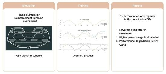
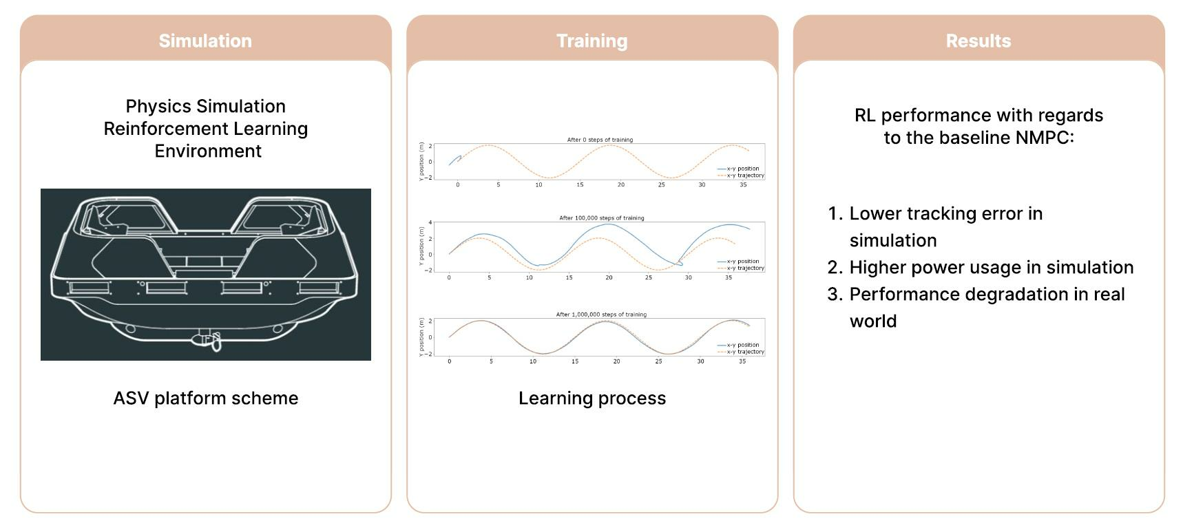
• Development of a comprehensive physical simulation for an ASV in urban waterways, including the modeling of the various disturbances and uncertainties affecting the platform based on a review of the relevant literature.
• Development of a deep reinforcement learning wrapper of the physical simulation in a standard learning environment and an end-to-end learning procedure modeled specifically with the task of trajectory tracking in urban waterways in mind.
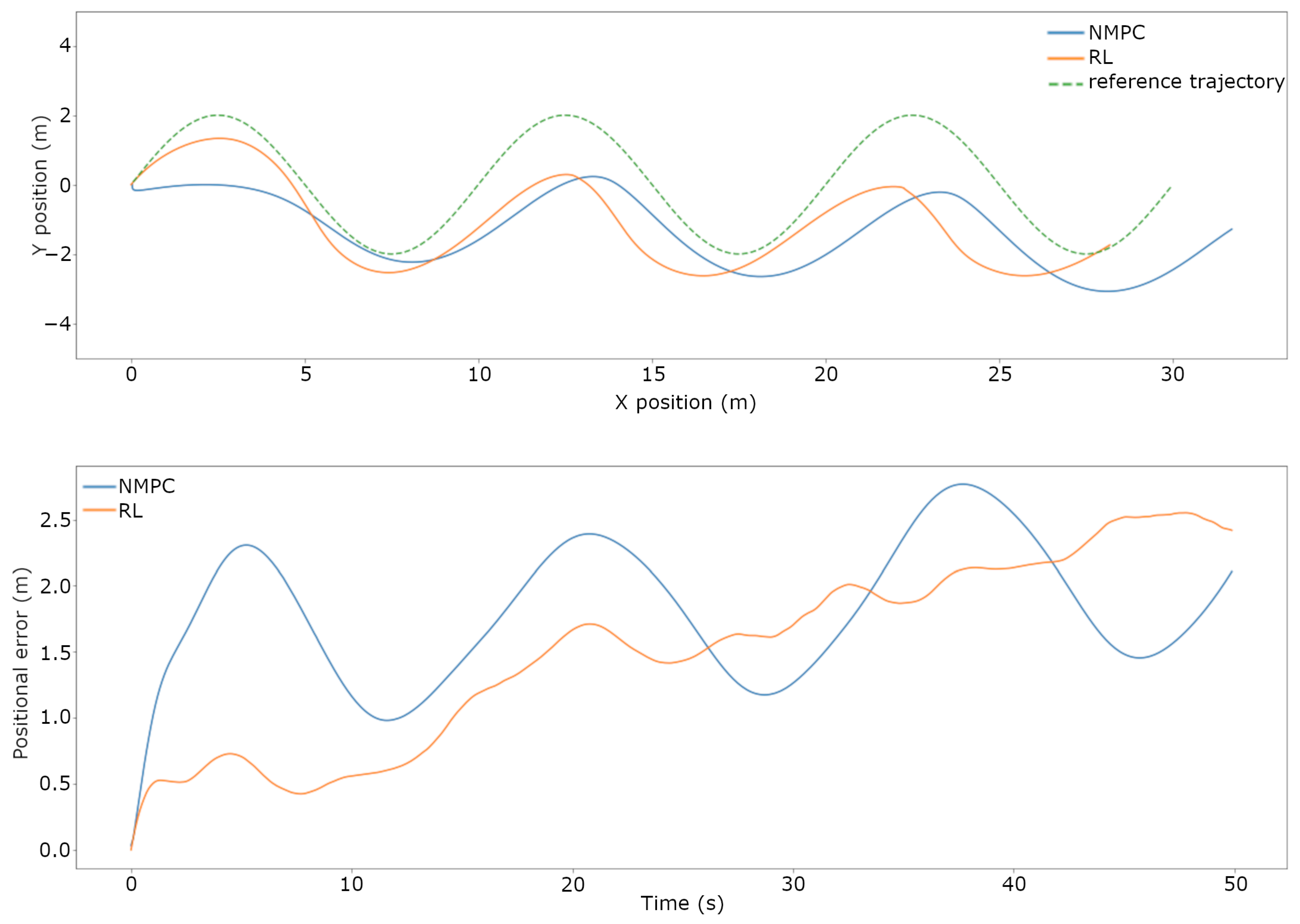
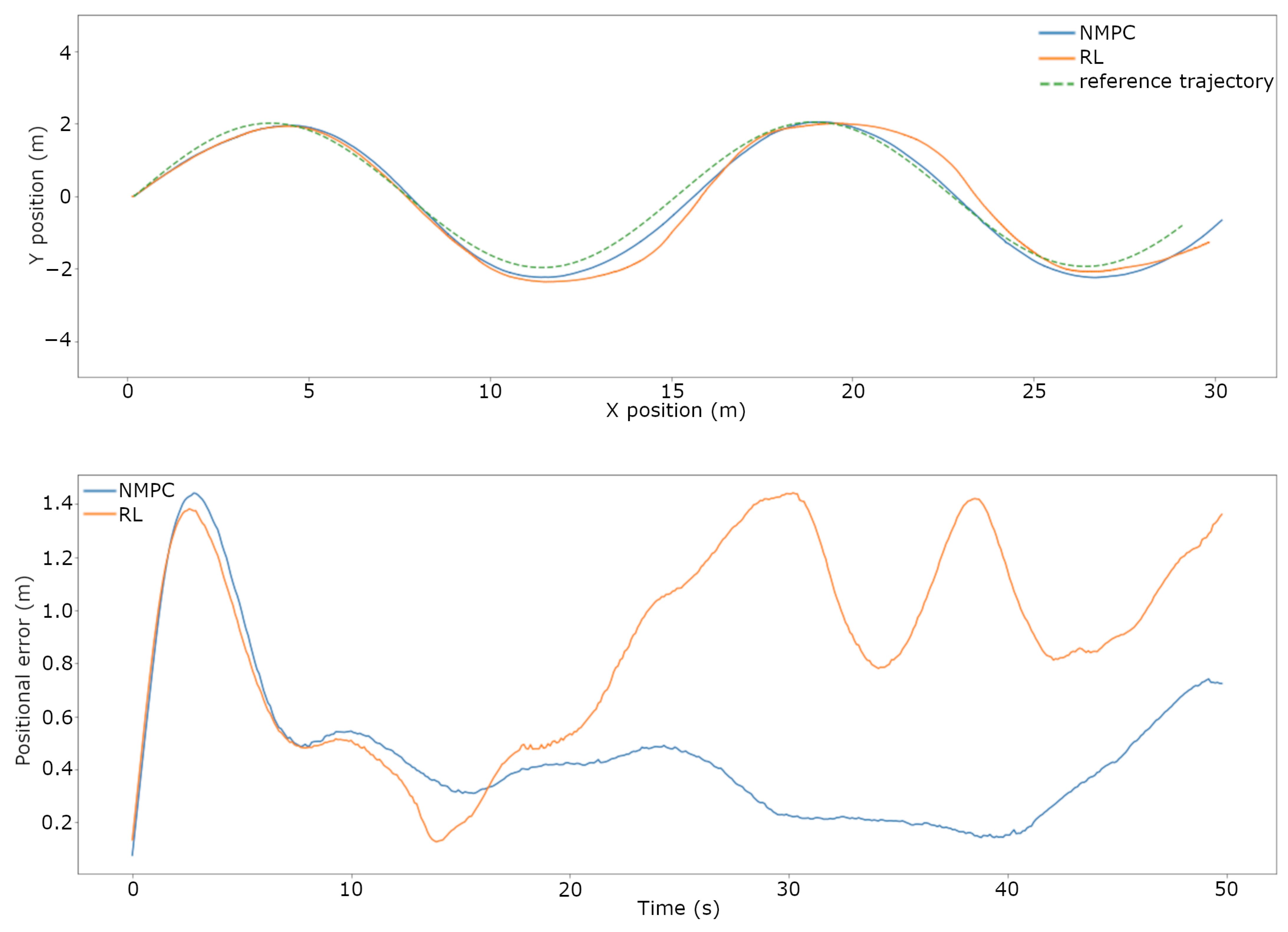
• A presentation of the rigorous testing procedure and the comparison between the current NMPC and the trained RL-based controller’s performance both in simulation and real-world scenarios. When subjected to disturbances and uncertainties, the RL-based controller was capable of performing trajectory tracking with a lower error than the current NMPC in a simulation, falling short in the real-world scenario.

The document is divided into the following parts. Firstly, an introduction of the problem at hand is given, as well as the literature focusing on related topics. Secondly, an overview of the theory behind the kinematics and dynamics of ASVs and reinforcement learning is provided. Furthermore, a description of the process of simulating the problem setting and designing an RL-based controller is given. Thirdly, the results of the comparison between the developed controller and the current control strategy are presented. And finally, the document ends in a discussion of the results and a conclusion of the study.

2. Materials and Methods

In this section, the theoretical background behind the key ideas of this study will be provided. Firstly, the fundamental concepts behind vessel kinematics and dynamics will be presented. Secondly, a short introduction of the reinforcement learning (RL) methods related to this work will be given. And thirdly, the interface between the ASV dynamics and the RL algorithm will be explained.

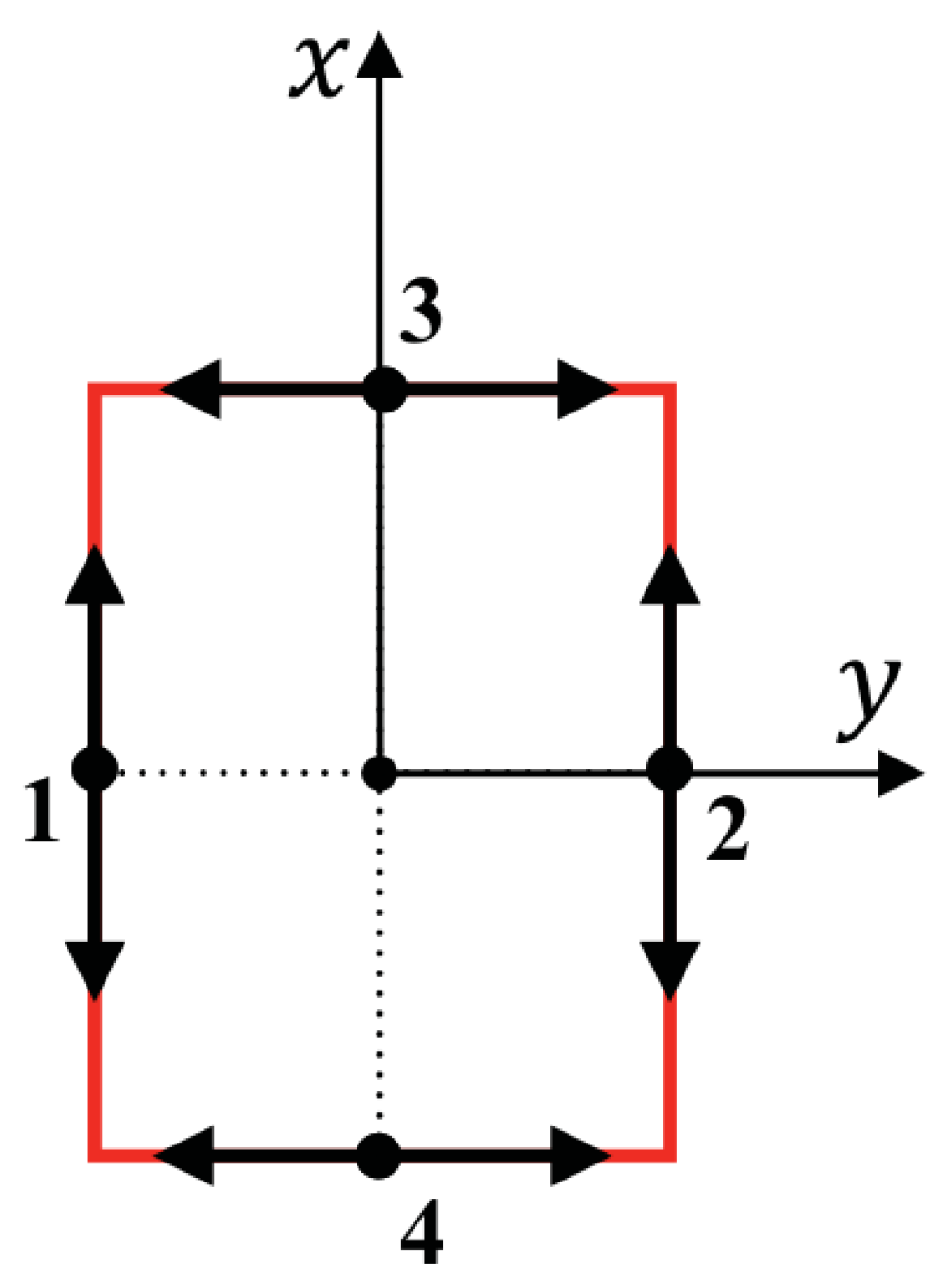
2.1. ASV Kinematics and Dynamics

The movement of an ASV can be expressed using two reference frames: the inertial and the vessel’s own reference frame. In the inertial reference frame, it can be condensed in a three-degrees-of-freedom (DOFs) vector $\mathit{\eta }$, presenting the vessel’s position (x and y) and orientation ($\psi$) [14]:

$$\mathit{\eta }=[x,y,\psi ]$$

(1)

Likewise, the linear (u in x and v in y direction) and angular velocities (r) of the vessel’s movement can be expressed in the vessel’s reference frame as a vector $\mathit{\nu }$:

$$\mathit{\nu }=[u,v,r]$$

(2)

The two vectors are related through the following equation:

$$\dot{\mathit{\eta }}=\mathit{R}\left(\psi \right)·\mathit{\nu }$$

(3)

where $\mathit{R}\left(\psi \right)$ is the transformation matrix from the vessel’s own to the inertial frame.

A popular form of propulsion for ASVs is propellers, which produce thrust $\mathsf{\tau }$ relative to the vessel’s advance speed and the propeller RPM with the following equations [14]:

$$\mathsf{\tau }=\rho D^4{K}_T\left(J_0\right)\left|u\right|u$$

(4)

$$J_0=\frac{(1-\omega )\mathit{\nu }}{uD}$$

(5)

where $\rho$ is the density of the fluid, D the propeller diameter, $K_T$ the thrust coefficient estimated for a hull–propeller pairing, $J_0$ the advance number, defined with Equation (5), and $\omega$ the wake fraction number.

The Roboat platform is actuated through a set of four thrusters in the “+” thruster configuration, with the main thrusters on the port and starboard side of the center of mass and two sideways thrusters on the bow and stern, as can be seen in Figure 1. This type of configuration makes the system overactuated and the resulting force allocation matrix of the system is defined as

$$\mathsf{\tau }=\mathit{Bu}=\left[\begin{array}{cccc}1& 1& 0& 0\\ 0& 0& 1& 1\\ \frac{a}{2}& -\frac{a}{2}& \frac{b}{2}& -\frac{b}{2}\end{array}\right]\left[\begin{array}{c}{f}_1\\ f_2\\ f_3\\ f_4\end{array}\right]$$

(6)

where a and b are the vessel’s width and length, while $f_i$ (i = 1,2,3,4) are the thruster forces.

Among other things, ASVs in urban waterways are affected by the following uncertainties and disturbances: varying payload, wind, and current. These can be modeled in the following manner.

Firstly, if the magnitude of the payload is significant with regard to the vessel’s own weight, a varying payload induces a high trajectory tracking error. The effect of the distribution and magnitude of the payload is reflected in a proportional change in the vessel’s mass and damping matrices and the wake fraction number $\omega$ [14].

Secondly, the effect of wind can be approximated with a force and torque combination ${\mathsf{\tau }}_{\mathit{w}}$ acting on the vessel with

$${\mathsf{\tau }}_{\mathit{w}}=\frac{1}{2}{\rho }_a{V}_{rw}^2\left[\begin{array}{c}-c_x{A}_{FW}cos\left({\gamma }_{rw}\right)\\ c_y{A}_{LW}sin\left({\gamma }_{rw}\right)\\ c_z{A}_{LW}{L}_{OA}sin\left(2{\gamma }_{rw}\right)\end{array}\right]$$

(7)

where ${\gamma }_{rw}$ is the apparent wind angle, ${\rho }_a$ the density of air, $V_{rw}$ the apparent wind speed, $A_{FW}$ the frontal projected windage area, $A_{LW}$ the lateral projected windage area, and $L_{OA}$ the vessel’s overall length. $c_x$, $c_y$, and $c_z$ are the wind coefficients estimated for the vessel at hand.

Thirdly, the current acts as a constant translation of the vessel’s moving frame with a certain velocity [14]:

$$u_c=V_{c}cos(\beta -\psi )$$

(8)

$$v_c=V_{c}cos(\beta -\psi )$$

(9)

where $u_c$ and $v_c$ present the current’s velocity in the vessel’s surge and sway directions, respectively, $V_c$ the speed of the current, and $\beta -\psi$ the current’s angle of attack on the vessel.

Finally, the equations of motion for the entire system can be written as

$$\mathit{M}\dot{\mathit{\nu }}+\mathit{C}\left(\mathit{\nu }\right)\mathit{\nu }+{\mathit{D}}_{\mathit{L}}\left(\mathit{\nu }\right)\mathit{\nu }+\mathit{\nu }{\mathit{D}}_{\mathit{Q}}\left(\mathit{\nu }\right)\mathit{\nu }+\mathit{g}\left(\mathit{\eta }\right)=\mathsf{\tau }$$

(10)

$$\mathit{M}={\mathit{M}}_{\mathit{RB}}+{\mathit{M}}_{\mathit{A}}$$

(11)

$$\mathsf{\tau }={\mathsf{\tau }}_{\mathit{u}}+{\mathsf{\tau }}_{\mathit{E}}$$

(12)

where ${\mathit{M}}_{\mathbf{RB}}+{\mathit{M}}_{\mathit{A}}$ are the rigid body and added mass terms, ${\mathit{D}}_{\mathit{L}}\left(\mathit{\nu }\right)$ the linear damping matrix, ${\mathit{D}}_{\mathit{Q}}\left(\mathit{\nu }\right)$ the quadratic damping matrix, ${\mathsf{\tau }}_{\mathit{u}}$ the vector of thruster-generated torques, and ${\mathsf{\tau }}_{\mathit{E}}$ the vector of environmental torques [14].

2.2. Reinforcement Learning

Basic reinforcement learning problems can be described through the notion of discrete-time stochastic control processes called Markov decision processes (MDPs) [29]. An MDP consists of a tuple $(S,A,P_a,R_a)$, with the following components:

• S is the set of possible states called the state space;
• A is the set of possible actions called the action space;
• $P_a$ is the probability of action a taken in state s leading to state $s^{\prime }$;
• $R_a$ is the immediate reward for taking action a in state s.

The agent’s behavior, or more precisely the choice of action in any given state, is defined through the policy function $\pi (s,a)$. A policy that maximizes the reward function in the infinite horizon is called the optimal policy ${\pi }^{*}(s,a)$. The goal of RL algorithms is to obtain this optimal policy for a given agent–environment pair [29].

A family of reinforcement learning algorithms called policy gradient methods showed promise by presenting the policy ${\pi }_{\theta }(s,a)$ as a parametrized probability distribution (e.g., a neural network), optimized through gradient ascent on the expected reward, obtained by following that ${\pi }_{\theta }(s,a)$. This is usually achieved by using the gradient estimator $\widehat{g}$ Equation (13), obtained by differentiating the loss function $L^{PG}$ Equation (14), and following the update rule Equation (15).

$$\widehat{g}={\widehat{\mathbb{E}}}_t\left[{\nabla }_{t}log{\pi }_{\theta }\left(a_t\right|s_t){\widehat{A}}_t\right]$$

(13)

$$L^{PG}\left(\theta \right)={\widehat{\mathbb{E}}}_t\left[log{\pi }_{\theta }\left(a_t\right|s_t){\widehat{A}}_t\right]$$

(14)

$${\theta }_{new}={\theta }_{old}+\alpha \widehat{g}$$

(15)

where:

• $log{\pi }_{\theta }\left(a_t\right|s_t)=$ the log probability of the output of the policy ${\pi }_{\theta }$ in state $s_t$;
• ${\widehat{A}}_t=$ the estimator of the relative value taking the selected action at time t with regard to the old policy, called the advantage function;
• $\alpha =$ the learning rate.

At the time of writing, the most recent breakthrough in the family is the proximal policy optimization (PPO) from [28]. Presented in 2017, PPO is simple, more general than its predecessors, and has better sample complexity. To achieve this performance, the algorithm uses two tricks: trust region methods [30] and a clipped surrogate objective.

The PPO algorithm improves on its predecessors TRPO [30] and ACER [31] by using the following two approaches: trust region methods and a clipped surrogate objective. Firstly, trust region methods optimize the policy by using a surrogate objective (16) to make small improvements on the policy chosen from a small region around the current policy called the trust region.

$$\underset{\theta }{max}{\widehat{\mathbb{E}}}_t\left[\frac{{\pi }_{\theta }(a_t,s_t)}{{\pi }_{{\theta }_{old}}(a_t,s_t)}{\widehat{A}}_t\right]={\widehat{\mathbb{E}}}_t\left[r_t\left(\theta \right){\widehat{A}}_t\right]$$

(16)

where:

• ${\pi }_{\theta }(a_t,s_t),{\pi }_{{\theta }_{old}}(a_t,s_t)=$ the new and old policy functions;
• ${\widehat{A}}_t=$ the estimator of the relative value of a selected action at time t, called the advantage function.

Secondly, the clipped surrogate objective function (17) is used to constrain the policy update by weighing the advantage of the update to the size of the update.

$$L^{CLIP}\left(\theta \right)={\widehat{\mathbb{E}}}_t\left[min(r_t\left(\theta \right){\widehat{A}}_t,clip(r_t\left(\theta \right),1-ϵ,1+ϵ){\widehat{A}}_t)\right]$$

(17)

where:

• $ϵ=$ a hyperparameter, for example, 0.2;
• $clip(r_t\left(\theta \right),1-ϵ,1+ϵ)=$ modifies the surrogate objective by clipping the probability ratio;
• $r_t\left(\theta \right)=$ immediate reward at time t.

PPO offers a versatile and robust learning process, less computationally intensive than its predecessors while retaining their stability and reliability.

2.3. Simulation of the Roboat and Design of the RL Controller

To simulate the Roboat system in code, a thorough research of the available ASV simulation tools was conducted. However, as no adequate simulator was found in the process, the simulator was built as part of this work. To this end, the equations from Section 2.1 were translated into Python code, parameterized based on uncertainties and disturbances, and wrapped in a Gym environment, following the interface architecture from the industry standard OpenAI Gym [32].

The software for the Roboat platform is built in the ROS framework and its architecture is given in Figure 2. To make use of a controller obtained through the training process, a new ROS node was developed to communicate with the rest of the navigation stack. Due to the modular nature of the system’s architecture, switching between the NMPC and the RL-based controller was simple.

The following criteria must be met by the environment to use RL algorithms in it: the observation and action space must be defined, and the step and reset methods must be defined.

For the task of trajectory tracking, the observation space was chosen to contain (i) the x and y error in the vessel’s reference frame, (ii) the sine and cosine (for continuity) of the look-ahead heading error, (iii) the current and reference velocity values, and (iv) the actuation vector for the previous time step.

The action space was defined as four values, from −1 to 1, mapped to the minimum and maximum of the thruster output value range.

The reward function was defined as

$$r_t=\left\{\begin{array}{cc}\hfill r_{gauss}+r_{heading}-r_u-r_{\Delta u}\hfill & \hfill \mathrm{if}{\mathit{\eta }}_{\mathit{err}}\le 5\hfill \\ -100\hfill & \hfill \mathrm{if}{\mathit{\eta }}_{\mathit{err}}>5\hfill \end{array}\right.$$

(18)

where ${\mathit{\eta }}_{\mathit{err}}$ is the Euclidean position error.

The first term was designed using a multivariate Gaussian function to reward smaller errors in the Euclidean space:

$$r_{gauss}=exp\left(-k_1·({({\widehat{x}}_t-x_t)}^2+{({\widehat{y}}_t-y_t)}^2)\right)$$

(19)

The second term was designed to reduce the look-ahead heading error with a Gaussian function:

$$r_{heading}=exp\left(-k_2·{({\widehat{\psi }}_t-{\psi }_t)}^2\right)$$

(20)

where $\Delta {\mathit{\psi }}_{\mathit{t}}$ is the difference between the current and desired heading at time t. This term was found to improve the actuation smoothness, as the RL algorithm learned to rely on the main thrusters more, leading to steadier trajectories.

Understanding the reward values throughout the system’s observation space can be difficult, so to gain a better understanding of the multivariate Gaussian terms in the reward function Figure 3 and Figure 4 offer a 3D plot and a 2D contour plot. From the figures it is clear that this, being the most significant part of the reward function, rewards proximity to the goal position within a radius of around 1 m, with a look-ahead heading error less than 0.5 radians.

The third term is designed to punish high actuation values:

$$r_u=k_3·\left(k_5·(u_{1,t}^2+u_{2,t}^2)+k_6·(u_{3,t}^2+u_{4,t}^2)\right)$$

(21)

where $u_{i,t}(i=1,2,3,4)$ are the actuation values at time t.

And lastly, the fourth term punishes high variations between consecutive actuation values for each of the thrusters, to improve smoothness and reduce wear and tear:

$$r_{\Delta u}=k_4·\sum _{i=1}^4\left|(u_{i,t}-u_{i,t-1})\right|$$

(22)

Introducing terms similar to the last two is common practice when deploying RL algorithms to the real world, as it avoids learning extreme actuation policies such as the bang–bang controller [24,33].

The constant parameters $k_i(i=1,\dots ,6)$ play a crucial role in balancing the impact of each component of the learning process. The specific values used in this study are listed in

Table 1. Constant values in the reward function.

Parameter	${\mathit{k}}_1$	${\mathit{k}}_2$	${\mathit{k}}_3$	${\mathit{k}}_4$	${\mathit{k}}_5$	${\mathit{k}}_6$
Value	3	3	1	0.5	0.1	0.7

. An optimal search for the values was not feasible due to the high computation cost of training. Rather, the parameter values have been found through a heuristically guided search, based on the trade-off between tracking performance and smooth actuation.

The RL simulator was also compared to the proprietary Roboat simulation through step-response tests, which validated that it performs almost identically to the proprietary one.

To provide the algorithm with a diverse set of trajectories for learning, a trajectory generation module was built to output straight line, circular, and sine wave trajectories. These were parameterized with speed, radius, amplitude, and period values to present a wide range of difficulties to the learning algorithm.

In this work, the PPO algorithm [28] was chosen to train a controller for the Roboat platform in the simulation, as it currently outperforms similar algorithms in a number of control related tasks [30].

In this study, the neural network representing the agent consisted of two fully connected layers with 64 neurons each. The input of the network was a 14 value vector representing the observation space, and the output of the network was a vector of four values in the $[-1,1]$ range. These values were then scaled to the thruster’s actual force output allocation range.

3. Results

In order to obtain the best performance, the effect of changing PPO’s hyperparameters such as the learning rate, batch size, discount factor, whether to use generalized state-dependent exploration (gSDE), etc., was studied. Through this process, the optimal combination of hyperparameters was found to be those shown in

Table 2. PPO algorithm hyperparameters.

Parameter	Learning Rate	N Steps per Update	Batch Size	N Epochs	Discount Factor	Use gSDE
Value	0.0003	2048	256	10	0.99	False

.

It should be noted that, in the end, keeping the default values for most of the hyperparameters yielded the best results.

The network training was conducted for approximately 1 million time steps. It was observed that, at this point, the performance improvement plateaued, indicating signs of overfitting. For better understanding, the evolution of the episodic reward through the training process can be observed in Figure 5 and the learning process itself is visualized in Figure 6 on a sine wave trajectory.

Having trained a trajectory tracking controller it was time to compare it to the current control strategy. The performance of the NMPC and the RL controller was compared through two metrics. Firstly, the tracking precision was compared with the root mean squared error (RMSE) of the Euclidean distance between the current position and the desired position on the reference trajectory. Secondly, the average power usage of a given algorithm was measured using Equation (23):

$$P_{average}=\sum _{i=1}^N\frac{\left(\right|f_1^i|+|f_2^i|+|f_3^i|+|f_4^i\left|\right)·|u^i|}{N}$$

(23)

where N is the number of data points, $u^i$ is the surge speed of the vessel at time i, and $f_j^i$ is the force command for thruster j at time i. To conduct a thorough study of the performance of the trained controller with regards to the current NMPC approach, the behavior of the two controllers was examined in the following settings:

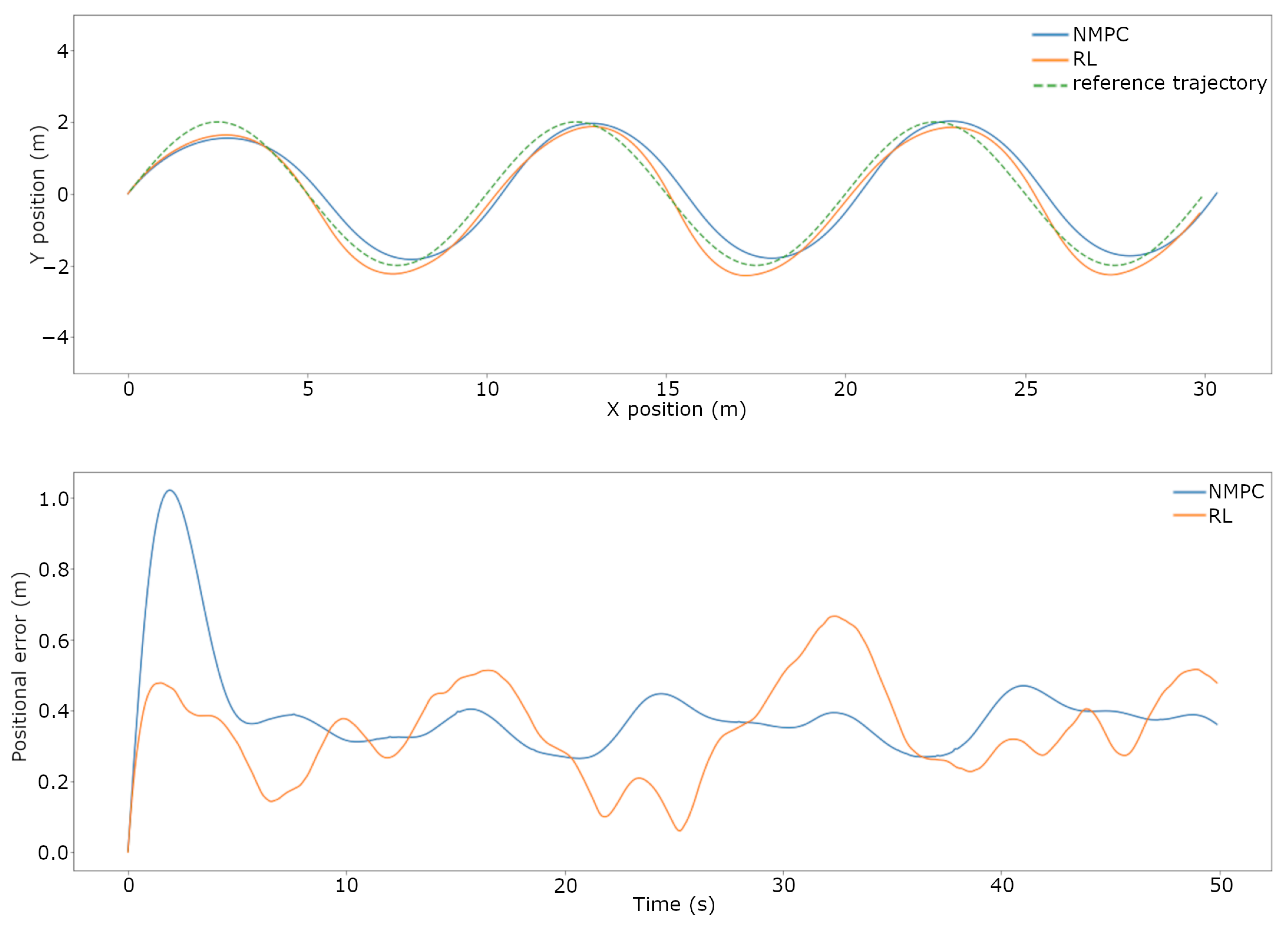
• Scenario 1—Baseline: without uncertainties and disturbances;
• Scenario 2—Payload: with a significant payload;
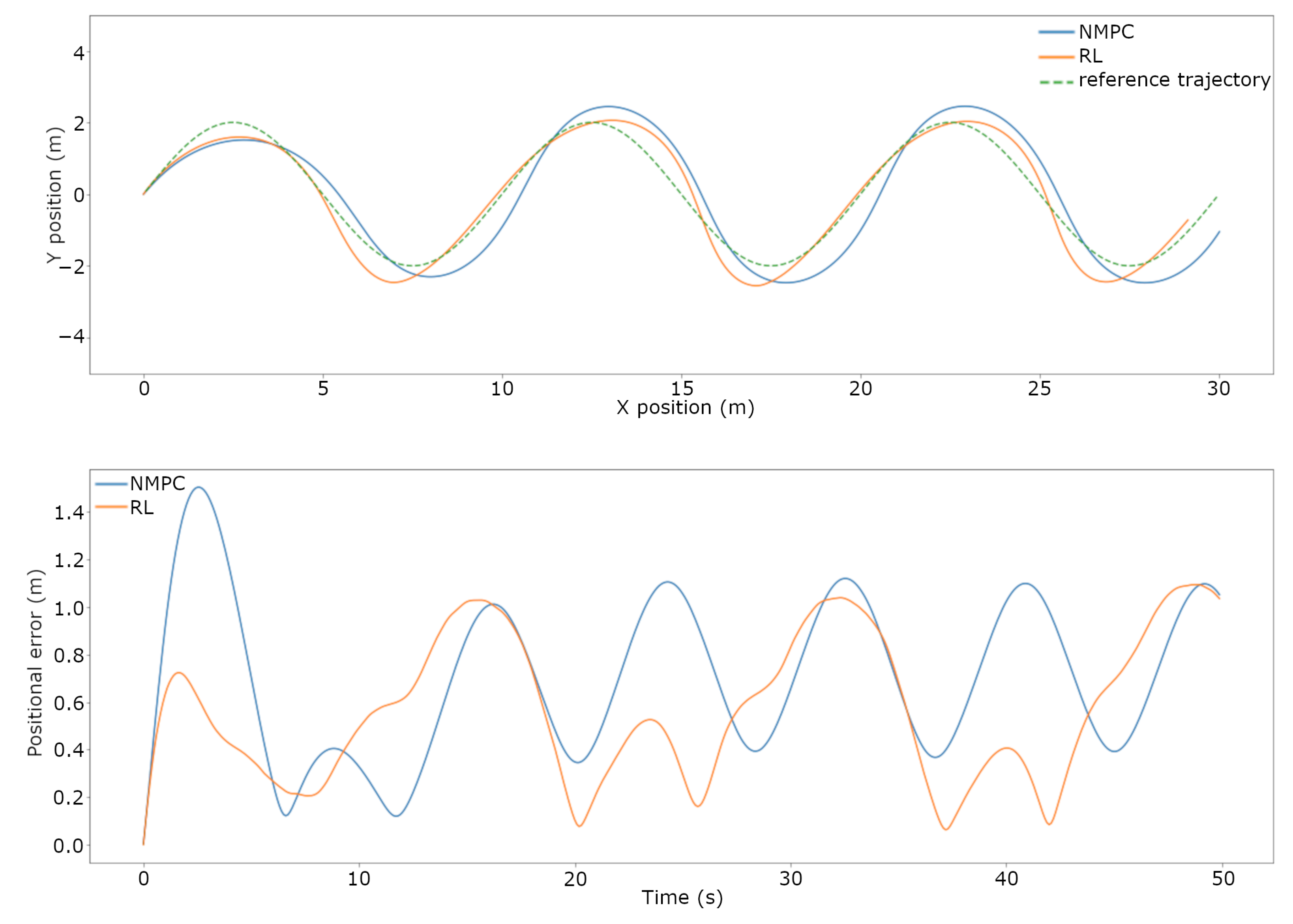
• Scenario 3—Current: facing a current disturbance;
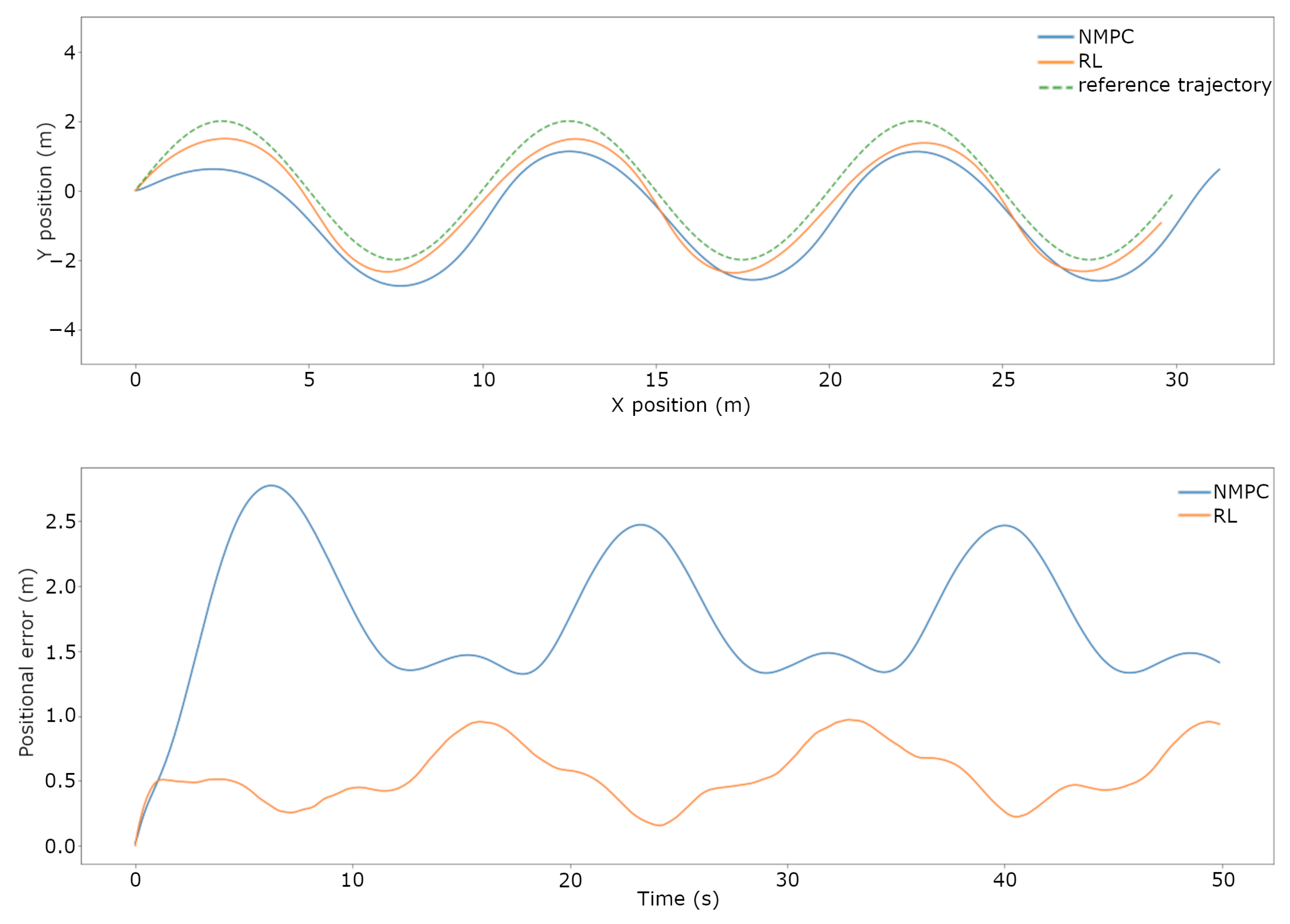
• Scenario 4—Wind: facing a wind disturbance;
• Scenario 5—Real World: testing the controller on the real platform.

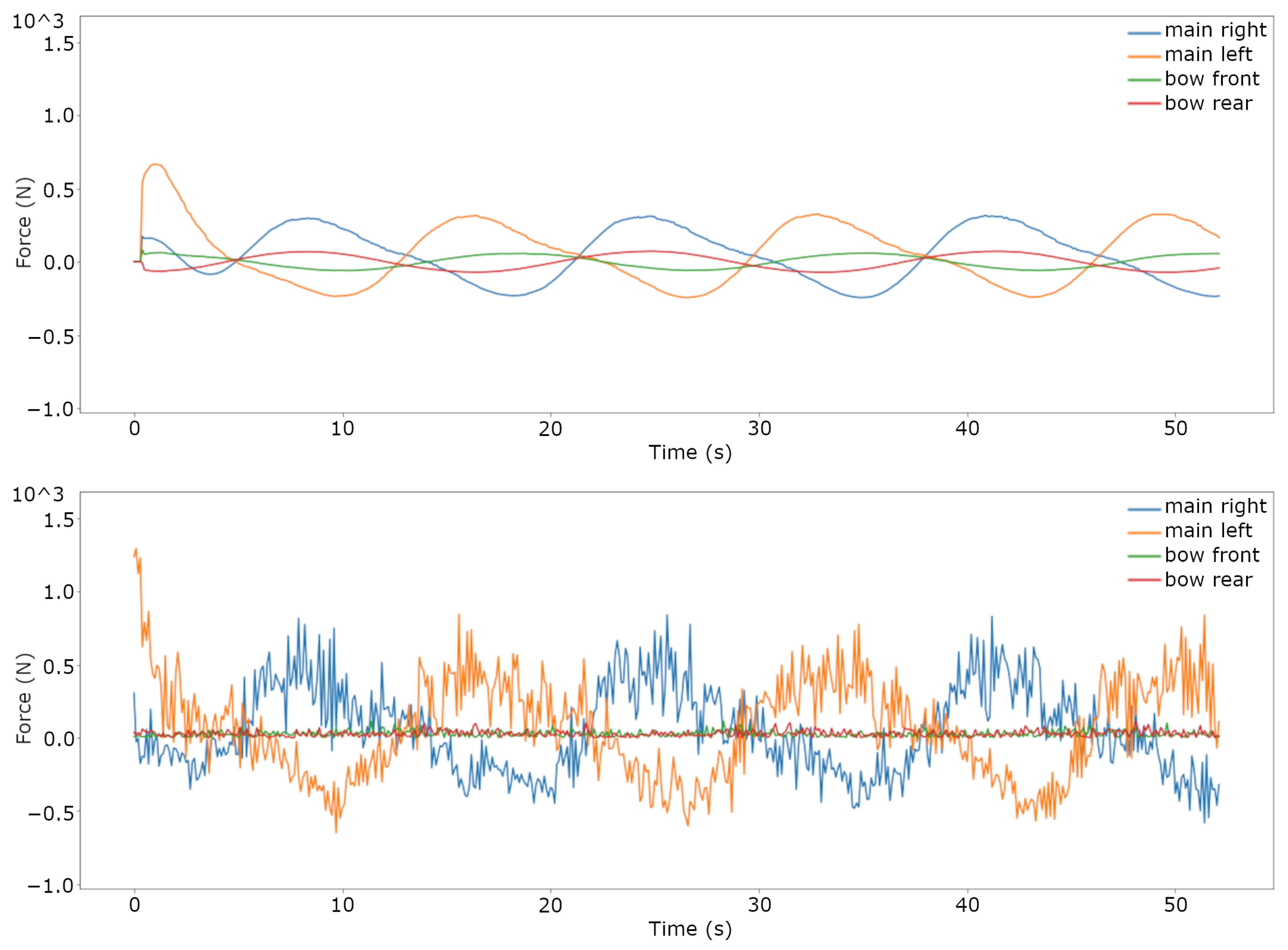
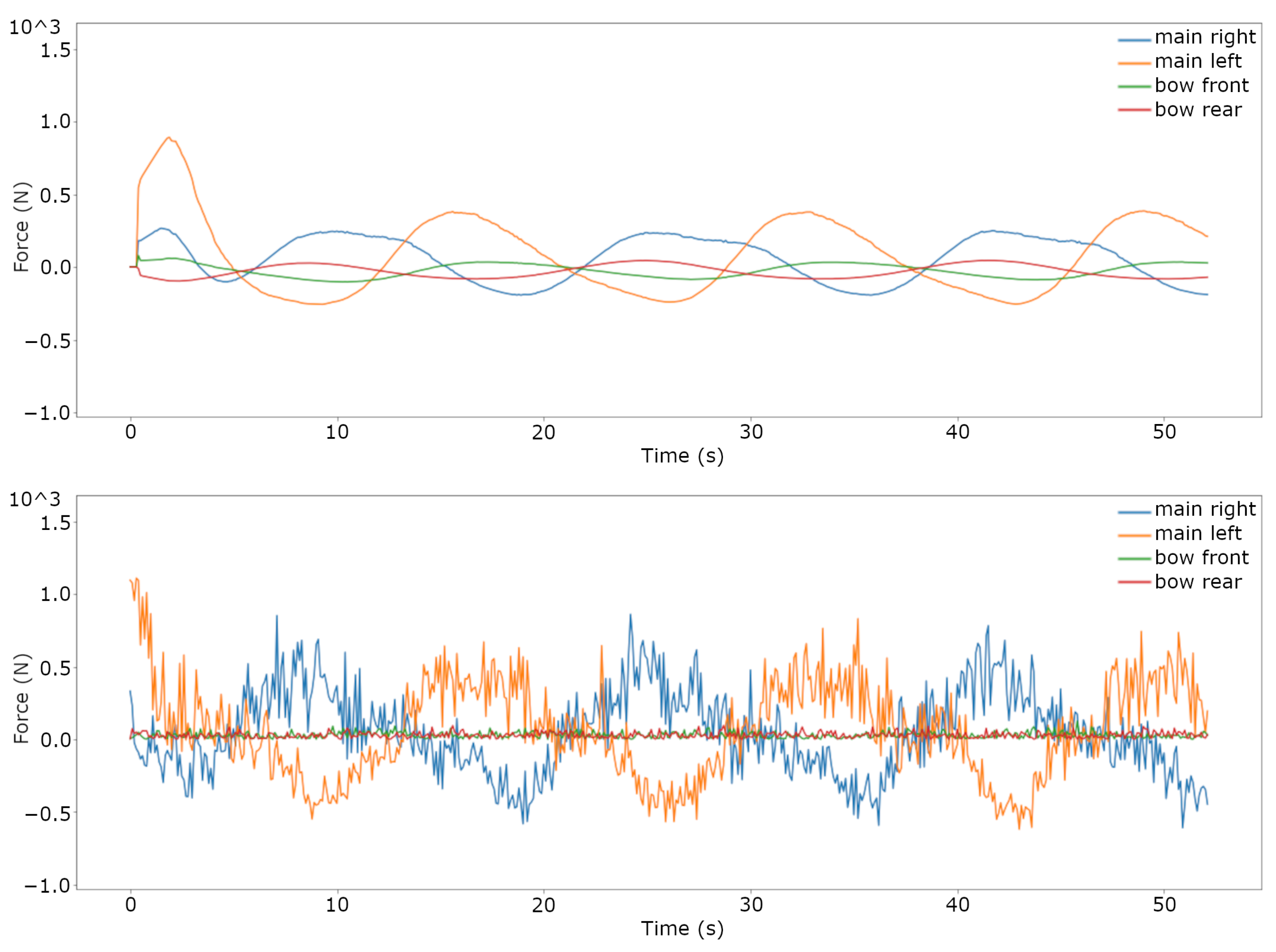
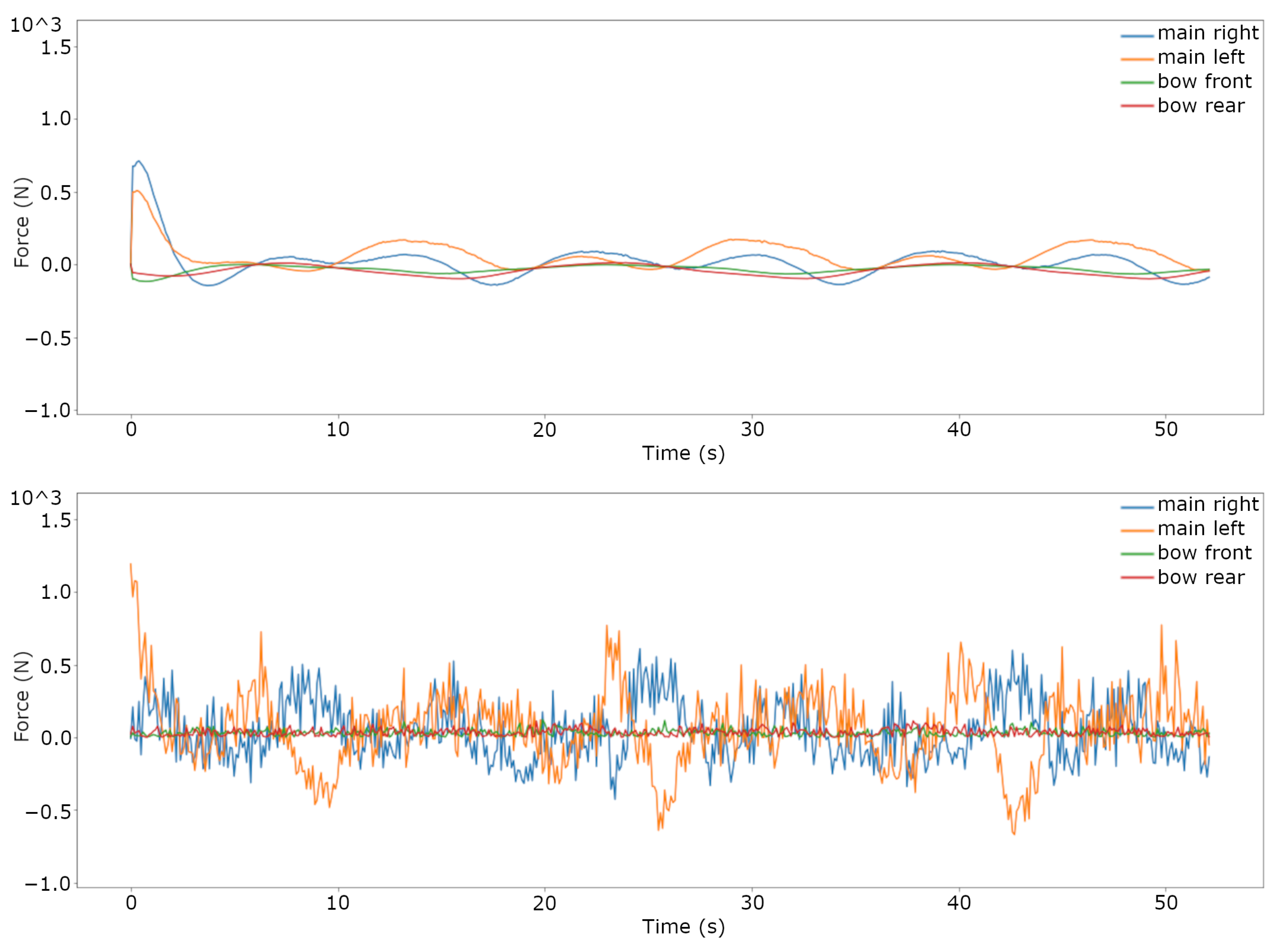
3.1. Trajectory Tracking Comparison in Simulation

The tests in the simulation were performed on a sine wave trajectory with the following parameters: amplitude = 2 m, period = 10 m, and forward speed = 0.5 m/s. Tracking such a trajectory presents both a realistic objective as well as a challenging task for the Roboat platform. The magnitude of the modeled uncertainties and disturbances has been carefully selected to depict the expected worst case scenarios for the Roboat platform.

Firstly, Figure 7 and Figure 8 visualize the results of the comparison between the simulations for scenario 1—baseline, without the inclusion of uncertainties and disturbances. The x–y position, tracking error through time, and force allocation through time are presented in the graphs. During this episode, the average positional error of the NMPC was 0.3018 m, whereas that of the RL-based controller was 0.2836 m. Putting these numbers in perspective, the RL-based controller performed better by 6.03%. When it comes to the power usage calculated by the aforementioned formula, the NMPC used on average 323.7134 W and the RL-based controller 491.3406 W of power. Relative to the NMPC, the RL-based controller algorithm used on average 51.78% more power.

Secondly, Figure 9 and Figure 10 visualize the results of the comparison between the simulations for scenario 2—payload, in which the system’s weight is increased by 50%. The figures are represented in the same manner as for the non-disturbed setting. Throughout the episode, the average positional error of the NMPC was 0.6979 m, while that of the RL-based controller was 0.5836 m, showing a 22.83% improvement with regards to the baseline NMPC. On the other hand, in terms of power usage, the NMPC used on average 559.3913 W and the RL-based controller 742.1449 W of power. The difference between the two in this case is 32.67% in favor of the NMPC.

Thirdly, Figure 11 and Figure 12 visualize the results of the same comparison of the system for scenario 3—current, with a current of 0.5 m/s acting on it. The introduction of a current disturbance to the system produced the following outcomes: the average positional error of the NMPC was 1.6810 m, whereas that of the RL-based controller was 0.5803 m. This time, the RL-based controller exhibited a very significant, 65.48% performance improvement over the NMPC. As for the power usage, the NMPC used on average 412.3100 W and the RL-based controller 460.2448 W of power, or an increase of 11.63%.

Finally, Figure 13 and Figure 14 visualize the results of the comparison in scenario 4—wind, with a wind speed of 9 m/s acting on the system. The wind disturbance induces the worst performance, with the average positional error of the NMPC being 1.8032 m and the RL-based controller 1.701 m, this being a 5.69% improvement with regards to the NMPC baseline, while the average power usage is 184.7790 W for the NMPC and 300.3304 W for the RL-based controller, which is 63.53% worse than the NMPC.

3.2. Trajectory Tracking Comparison on the Real System

After studying the controller in the simulation, the ROS framework needed for the deployment to the real system was developed. Upon deployment, a number of problems arose that caused failure. While some problems were resolved successfully, others were only partially mitigated.

Firstly, measurement noise and GPS delay caused choppy odometry signals which, as the RL-based controller was trained on a perfect odometry signal, led to performance deterioration. The odometry signal of the real system is calculated with an extended Kalman filter from an IMU and two GPS sensors. To mitigate the problem, the covariance matrix of the Kalman filter was re-tuned to obtain a smoother output.

Secondly, the most serious problem discovered was the discrepancy between the physical vessel and thruster model between the real world and the simulation. Upon careful inspection, the thruster behavior was discovered to be a compound problem formed of a 0.5–1 s command signal delay, a proprietary PID controller on the RPM value, and thruster dynamics (as explained in Section 2.1). These effects are most obvious whenever changing the propeller rotation direction, which is why the sine waves are tracked much worse in real life than in the simulations. This transient behavior is very difficult to model as the flow coming into the propeller is turbulent, not constant.

Furthermore, this led to errors in parameter estimation for the physical model as the reference force values do not align with the true output. Approaches used in the scope of this work to improve the model range from adding random noise, autoregressive, moving average processes, and thruster dynamic modeling. In the end, a combination of random noise added during training and a moving average with a window of size 5 (previous 0.5 s) applied to the actuation vector yielded the best results. The resulting actuation was more robust and the algorithm learned the slower and unreliable nature of the actuation. Detailed modeling of the thruster from a control signal to the actual thrust output could be a very interesting case study in itself.

Figure 15 and Figure 16 visualize the best results for the RL-based controller in scenario 5—real world, with two people on board, amounting to around 160 kg of additional payload, facing a frontal wind of around 2 on the Beaufort scale, and no notable current or waves. The RL-based controller also needed a head start from the NMPC to start the trajectory tracking for the first few seconds. Once again, the graphs present the position, the tracking error, and the force allocation.

Finally,

Table 3. Comparison between the NMPC and the RL algorithm in the evaluated metrics: average position error and power consumption.

Scenario	Undisturbed	Added Payload	Current	Wind	Real World
$\Delta$ pos. NMPC (m)	0.3018	0.6979	1.6810	1.8032	0.4587
$\Delta$ pos. RL (m)	0.2836	0.5836	0.5803	1.701	0.8721
Difference	−6.03%	−22.83%	−65.48%	−5.69%	90.10%
$\Delta$ P NMPC (W)	323.7134	559.3913	412.3100	184.7790	161.4688
$\Delta$ P RL (W)	491.3406	742.1449	460.2448	300.3304	543.6210
Difference	51.78%	32.67%	11.63%	62.53%	336.67%

contains a performance comparison between the controllers in all scenarios, with and without the inclusion of the disturbances and uncertainties as well as in the real world.

4. Discussion

The data clearly show that in the simulations the RL controller is capable of reducing the tracking error. However, this comes at a significant cost of power, as the RL algorithm attempts to overcompensate for errors, hinting at model exploitation. This seems to be an artifact of the simulated environment, where unlike in real life, instant force is available to the algorithm. The algorithm then learns to react to even the smallest of errors, reducing its robustness.

More precisely, in scenario 1—baseline, it can be observed from Figure 7 and Figure 8 that the two controllers perform similarly in terms of positional error throughout the episode, with the RL-based controller being more reactive to its increase. In terms of their actuation signal, the NMPC outputs a smooth signal, suiting the slow dynamics of the vessel, and the RL-based controller outputs a noisy and discontinuous signal. Unfortunately, this does not translate well to the real world, as can be seen in the later figures.

In scenario 2—payload, when significant payload is added to the vessel, as expected, the system becomes more sluggish and the task of trajectory tracking more difficult. This can be seen best in the amplitudes of the sine wave trajectories in Figure 9 and Figure 10, where overshooting can be seen. Both controllers still remain more or less capable of tracking the trajectory and once again the force signal output of the RL-based controller contains undesirable high oscillations.

Figure 11 and Figure 12 illustrate that in scenario 3—current, the nature of the effect of the current disturbance is different. Rather than overshooting on both sides, the platform stays on one side of the trajectory, fighting the current throughout the episode. It is visible that the RL-based controller cancels the current disturbance more successfully, reacting faster and with more force. This is confirmed by the numbers, having significantly less tracking error at a marginal increase in average power usage.

From Figure 13 and Figure 14, with strong wind acting on the system in scenario 4—wind, it is clear that both controllers fail at precise trajectory tracking, with the platform drifting further and further away from the reference throughout the episode. Put in numbers, although the RL-based controller performs marginally better, it cannot be said that either of them performs well. While they both attempt to change direction in sync with the goal trajectory, both of them drift away from it constantly, ending up far away from the final position. It is interesting, however, that the NMPC appears to utilize the rotating effect the wind has on the platform to turn without using power. This is obvious from the NMPC force allocation graph, where the controller mainly uses throttle for clockwise turns.

Ultimately, deploying the RL-based controller on the real system proved problematic. It only achieved some level of trajectory tracking capability after substantial interventions. At first sight, it would appear the trajectory is tracked perfectly fine judging by the top graph in Figure 15. However, looking at the evolution of the positional error in the bottom graph and Figure 16, it is clear that the RL-based controller struggles to keep up with and loses track of the trajectory fairly quickly in scenario 5—real world. There is a significant lag between the goal position and the vessel reaching that position. It is also striking how little effort it takes for the NMPC to perform the trajectory tracking, indicating that there is a lot to gain from moving the simulation closer to the real system.

Another interesting avenue of research in the future would be an attempt to separate the uncertainty and disturbance “sensing” from the control module by training a neural network to approximate the effect of the disturbances and uncertainties from a short history of the system state, and using that to inform the control module. A similar approach was attempted in [10], where information about foot slippage of a quadrupedal robot was extracted.

5. Conclusions

The goal of this work was to develop a learning-based controller for trajectory tracking for ASVs which, faced with uncertainties and disturbances, could track trajectories with less tracking error than the current NMPC method. This current method does not take the uncertainties and disturbances into account, as there is no way to directly measure them on the Roboat platform.

Not finding an adequate simulator, a new simulator of the vessel’s dynamics, including the uncertainties and disturbances, was developed to train agents using reinforcement learning algorithms.

After the search for the best setup and hyperparameters, an agent was trained with the PPO algorithm in the simulation to perform trajectory tracking successfully, even when faced with uncertainties and disturbances. Compared to the current NMPC method, although exhibiting a significant increase in power consumption and an erratic actuation signal, the controller clearly showed better tracking performance, having less tracking error.

When deployed on the real system its performance deteriorated, proving not to be robust to differences between the real world and the simulated system, especially the thruster model. This work can be extended in two directions. Firstly, a more accurate model of the system’s and the thruster dynamics is necessary to facilitate the ability of the simulation to model the real world. And lastly, the reinforcement learning framework could be used to “learn” to sense the uncertainties and disturbances from a short history of sensor data.

References

1. Curcio, J.; Leonard, J.; Patrikalakis, A. SCOUT—A low cost autonomous surface platform for research in cooperative autonomy. In Proceedings of the MTS/IEEE Oceans, Washington, DC, USA, 17–23 September 2005. [Google Scholar]
2. Paull, L.; Saeedi, S.; Seto, M.; Li, H. AUV navigation and localization: A review. IEEE J. Ocean. Eng. 2014, 39, 131–149. [Google Scholar] [CrossRef]
3. Dhariwal, A.; Sukhatme, G.S. Experiments in robotic boat localization. In Proceedings of the IEEE/RSJ International Conference on Intelligent Robots and Systems, San Diego, CA, USA, 29 October–2 November 2007. [Google Scholar]
4. Azzeria, M.N.; Adnanb, F.A.; Zaina, M.Z.M. Review of course keeping control system for unmanned surface vehicle. J. Teknologi 2015, 5, 11–20. [Google Scholar] [CrossRef]
5. Liu, Z.; Zhang, Y.; Yu, X.; Yuan, C. Unmanned surface vehicles: An overview of developments and challenges. Annu. Rev. Control 2016, 41, 71–93. [Google Scholar] [CrossRef]
6. Wang, W.; Gheneti, B.; Mateos, L.A.; Duarte, F.; Ratti, C.; Rus, D. Roboat: An Autonomous Surface Vehicle for Urban Waterways. In Proceedings of the 2019 IEEE/RSJ International Conference on Intelligent Robots and Systems (IROS), Macau, China, 3–8 November 2019; pp. 6340–6347. [Google Scholar]
7. Wang, W.; Shan, T.; Leoni, P.; Fernandez-Gutierrez, D.; Meyers, D.; Ratti, C.; Rus, D. Roboat II: A Novel Autonomous Surface Vessel for Urban Environments. In Proceedings of the 2020 IEEE/RSJ International Conference on Intelligent Robots and Systems (IROS), Las Vegas, NV, USA, 24 October 2020–24 January 2021. [Google Scholar]
8. Wang, W.; Fernández-Gutiérrez, D.; Doornbusch, R.; Jordan, J.; Shan, T.; Leoni, P.; Hagemann, N.; Schiphorst, J.K.; Duarte, F.; Ratti, C.; et al. Roboat III: An Autonomous Surface Vessel for Urban Transportation. J. Field Robot. 2023, 1–14. [Google Scholar] [CrossRef]
9. Wang, W.; Mateos, L.A.; Park, S.; Leoni, P. Design, Modeling, and Nonlinear Model Predictive Tracking Control of a Novel Autonomous Surface Vehicle. In Proceedings of the IEEE International Conference on Robotics and Automation (ICRA), Brisbane, Australia, 21–25 May 2018. [Google Scholar]
10. Lee, J.; Hwangbo, J.; Wellhausen, L.; Koltun, V.; Hutter, M. Learning quadrupedal locomotion over challenging terrain. Sci. Robot. 2020, 5, 47. [Google Scholar] [CrossRef] [PubMed]
11. Balchen, J.; Jenssen, N.; Mathisen, E.; Saelid, S. Dynamic Positioning of Floating Vessels Based on Kalman Filtering and Optimal Control. In Proceedings of the 19th IEEE Conference on Decision and Control including the Symposium on Adaptive Processes, Albuquerque, NM, USA, 10–12 December 1980; pp. 852–864. [Google Scholar]
12. Holzhüter, T. Lqg approach for the high-precision track control of ships. IEE Proc. Control Theory Appl. 1997, 144, 121–127. [Google Scholar] [CrossRef]
13. Fossen, T.; Paulsen, M. Adaptive feedback linearization applied to steering of ships. Model. Identif. Control Nor. Res. Bull. 1995, 14, 229–237. [Google Scholar] [CrossRef]
14. Fossen, T.I. Guidance and Control of Ocean Vehicles; Wiley: Hoboken, NJ, USA, 1994. [Google Scholar]
15. Fossen, T.I. A Survey on Nonlinear Ship Control: From Theory to Practice; IFAC: Aalborg, Denmark, 2000. [Google Scholar]
16. Zhang, L.; Qiao, L.; Chen, J.; Zhang, W. Neural-network-based reinforcement learning control for path following of underactuated ships. In Proceedings of the 5th Chinese Control Conference, Chengdu, China, 27–29 July 2016. [Google Scholar]
17. Woo, J.; Yu, C.; Kim, N. Deep reinforcement learning-based controller for path following of an unmanned surface vehicle. Ocean. Eng. 2019, 183, 155–166. [Google Scholar] [CrossRef]
18. Gonzalez-Garcia, A.; Barragan-Alcantar, D.; Collado-Gonzalez, I.; Garrido, L. Adaptive dynamic programming and deep reinforcement learning for the control of an unmanned surface vehicle: Experimental results. Control Eng. Pract. 2021, 111, 104807. [Google Scholar] [CrossRef]
19. Gonzalez-Garcia, A.; Castañeda, H.; Garrido, L. Usv Path-Following Control Based on Deep Reinforcement Learning and Adaptive Control; Global Oceans: Singapore; Gulf Coast, TX, USA, 2020. [Google Scholar]
20. Martinsen, A.B.; Lekkas, A.M. Straight-path following for underactuated marine vessels using deep reinforcement learning. In Proceedings of the 11th IFAC Conference on Control Applications in Marine Systems, Robotics, and Vehicles, Opatija, Croatia, 10–12 September 2018. [Google Scholar]
21. Martinsen, A.B.; Lekkas, A.M. Curved path following with deep reinforcement learning: Results from three vessel models. In Proceedings of the OCEANS 2018 MTS/IEEE Charleston, Charleston, SC, USA, 22–25 October 2018. [Google Scholar]
22. Wang, Y.; Tong, J.; Song, T.-Y.; Wan, Z.-H. Unmanned surface vehicle course tracking control based on neural network and deep deterministic policy gradient algorithm. In Proceedings of the 2018 OCEANS—TS/IEEE Kobe Techno-Oceans, Kobe, Japan, 28–31 May 2018. [Google Scholar]
23. Martinsen, A.B.; Lekkas, A.; Gros, S.; Glomsrud, J.; Pedersen, T. Reinforcement learning-based tracking control of usvs in varying operational conditions. Front. Robot. AI 2020, 7, 32. [Google Scholar] [CrossRef] [PubMed]
24. Øvereng, S.S.; Nguyen, D.T.; Hamre, G. Dynamic positioning using deep reinforcement learning. Ocean. Eng. 2021, 235, 109433. [Google Scholar] [CrossRef]
25. Chen, L.; Dai, S.-L.; Dong, C. Adaptive Optimal Tracking Control of an Underactuated Surface Vessel Using Actor–Critic Reinforcement Learning. IEEE Trans. Neural Netw. Learn. Syst. 2022, 1–14. [Google Scholar] [CrossRef] [PubMed]
26. Wei, Z.; Du, J. Reinforcement learning-based optimal trajectory tracking control of surface vessels under input saturations. Int. J. Robust Nonlinear Control 2023, 33, 3807–3825. [Google Scholar] [CrossRef]
27. Martinsen, A.B.; Lekkas, A.M.; Gros, S. Reinforcement learning-based NMPC for tracking control of ASVs: Theory and experiments. Control Eng. Pract. 2022, 120, 105024. [Google Scholar] [CrossRef]
28. Schulman, J.; Wolski, F.; Dhariwal, P.; Radford, A.; Klimov, O. Proximal Policy Optimization Algorithms. arXiv 2017, arXiv:1707.06347v2. [Google Scholar]
29. Russell, S.; Norvig, P. Artificial Intelligence: A Modern Approach, 3rd ed.; Prentice Hall Press: Saddle River, NJ, USA, 2009. [Google Scholar]
30. Schulman, J.; Levine, S.; Abbeel, P.; Jordan, M.; Proceedings, P.M. Trust Region Policy Optimization. In Proceedings of the 32nd International Conference on Machine Learning, Lille, France, 6–11 July 2015. [Google Scholar]
31. Wang, Z.; Bapst, V.; Heess, N.; Mnih, V.; Munos, R.; Kavukcuoglu, K.; de Freitas, N. Sample Efficient Actor-Critic with Experience Replay. arXiv 2017, arXiv:1707.06347. [Google Scholar]
32. Brockman, G.; Cheung, V.; Pettersson, L.; Schneider, J.; Schulman, J.; Tang, J.; Zaremba, W. Openai gym. arXiv 2016, arXiv:1606.01540. [Google Scholar]
33. Mysore, S.; Mabsout, B.; Mancuso, R.; Saenko, K. Regularizing Action Policies for Smooth Control with Reinforcement Learning. arXiv 2021, arXiv:2012.06644. [Google Scholar]
Figure 1. Roboat platform “+” thruster configuration.
Computation 11 00216 g001
Figure 2. Structure of the Roboat platform architecture.
Computation 11 00216 g002
Figure 3. Visualization of Gaussian terms in the reward function in a 3D plot.
Computation 11 00216 g003
Figure 4. A contour plot of Gaussian terms in the reward function.
Computation 11 00216 g004
Figure 5. Plot of the episodic reward throughout one million steps of training. Orange line presents the moving average with a window size 50; light orange presents the standard deviation of the value.
Computation 11 00216 g005
Figure 6. Visualization of intermediate trajectory tracking training results for the RL controller upon initialization: 100,000, 200,000, 500,000, and 1,000,000 training steps.
Computation 11 00216 g006
Figure 7. Scenario 1—baseline. Comparison between the NMPC and RL algorithm trajectory tracking performance. Trajectories of NMPC, RL, and reference sine wave on the top graph. Tracking errors of NMPC and RL on the bottom graph.
Computation 11 00216 g007
Figure 8. Scenario 1—baseline. Comparison between the NMPC and RL algorithm trajectory tracking performance. Force allocation of NMPC (top graph) and RL (bottom graph) for tracking the sine wave trajectory.
Computation 11 00216 g008
Figure 9. Scenario 2—payload. Comparison between the NMPC and RL algorithm trajectory tracking performance with payload equal to 50% of vessel’s mass. Trajectories of NMPC, RL, and reference sine wave on the top graph. Tracking errors of NMPC and RL on the bottom graph.
Computation 11 00216 g009
Figure 10. Scenario 2—payload. Comparison between the NMPC and RL algorithm trajectory tracking performance with payload equal to 50% of vessel’s mass. Force allocation of NMPC (top graph) and RL (bottom graph) for tracking the sine wave trajectory.
Computation 11 00216 g010
Figure 11. Scenario 3—current. Comparison between the NMPC and RL algorithm trajectory tracking performance with a current of 0.5 m/s acting on the system. Trajectories of NMPC, RL, and reference sine wave on the top graph. Tracking errors of NMPC and RL on the bottom graph.
Computation 11 00216 g011
Figure 12. Scenario 3—current.Comparison between the NMPC and RL algorithm trajectory tracking performance with a current of 0.5 m/s acting on the system. Force allocation of NMPC (top graph) and RL (bottom graph) for tracking the sine wave trajectory.
Computation 11 00216 g012
Figure 13. Scenario 4—wind. Comparison between the NMPC and RL algorithm trajectory tracking performance with a wind of speed 9 m/s acting on the system. Trajectories of NMPC, RL, and reference sine wave on the top graph. Tracking errors of NMPC and RL on the bottom graph.
Computation 11 00216 g013
Figure 14. Scenario 4—wind. Comparison between the NMPC and RL algorithm trajectory tracking performance with a wind of speed 9 m/s acting on the system. Force allocation of NMPC (top graph) and RL (bottom graph) for tracking the sine wave trajectory.
Computation 11 00216 g014
Figure 15. Scenario 5—real world. Comparison between the NMPC and RL algorithm trajectory tracking performance on the real Roboat vessel. Trajectories of NMPC, RL, and reference sine wave on the top; tracking errors of NMPC and RL on the bottom.
Computation 11 00216 g015
Figure 16. Scenario 5—real world. Comparison between the NMPC and RL algorithm trajectory tracking performance on the real Roboat vessel. Force allocation of NMPC (top graph) and RL (bottom graph).
Computation 11 00216 g016