Global Properties of Cytokine-Enhanced HIV-1 Dynamics Model with Adaptive Immunity and Distributed Delays

Abstract

In this paper, we study a model that enhances our understanding of cytokine-influenced HIV-1 infection. The impact of adaptive immune response (cytotoxic T lymphocytes (CTLs) and antibodies) and time delay on HIV-1 infection is included. The model takes into account two types of distributional delays, (i) the delay in the HIV-1 infection of CD4⁺T cells and (ii) the maturation delay of new virions. We first investigated the fundamental characteristics of the system, then found the system’s equilibria. We derived five threshold parameters, ${\Re }_i$, i = 0, 1,…, 4, which completely determine the existence and stability of the equilibria. The Lyapunov method was used to prove the global asymptotic stability for all equilibria. We illustrate the theoretical results by performing numerical simulations. We also performed a sensitivity analysis on the basic reproduction number ${\Re }_0$ and identified the most-sensitive parameters. We found that pyroptosis contributes to the number ${\Re }_0$, and then, neglecting it will make ${\Re }_0$ underevaluated. Necrosulfonamide and highly active antiretroviral drug therapy (HAART) can be effective in preventing pyroptosis and at reducing viral replication. Further, it was also found that increasing time delays can effectively decrease ${\Re }_0$ and, then, inhibit HIV-1 replication. Furthermore, it is shown that both CTLs and antibody immune responses have no effect on ${\Re }_0$, while this can result in less HIV-1 infection.

1. Introduction

In the early 1980s, human immunodeficiency virus type-1 (HIV-1) was discovered. Since then, the virus has spread throughout the world and is considered one of the most-serious public health, social, and economic challenges in the world. The World Health Organization reported that, at the end of 2022, there were about 39-million people living with HIV-1 in the world [1]. The virus targets the immune system, especially CD4${}^{+}$T cells, which play an essential role in the immune system response to viruses. Acquired immune deficiency syndrome (AIDS) is the most-advanced stage of the disease. Untreated HIV-1-infected patients usually spend many years before reaching the AIDS stage. During this period, the CD4${}^{+}$T cell count declines slowly and reaches below 200 cells/mm${}^3$ [2].

During the last few decades, scientists and researchers from all fields have united their massive efforts to study and understand the mechanism between HIV-1 and target cells. The experimental evaluation of the interactions between HIV-1, CD4${}^{+}$T cells, and other immune cells can be difficult and expensive. Mathematical modeling can be very useful in understanding the dynamic behavior of HIV-1 in the host. This also helps in understanding the effectiveness of medications, whether individually or in combination. Nowak and Bangham [3] constructed a basic model for within-host HIV-1 dynamics. The model describes the interaction of three populations, uninfected CD4${}^{+}$T cells, infected CD4${}^{+}$T cells, and free HIV-1 particles, as:

$$\begin{array}{cc}\hfill \mathrm{Uninfected}{\mathrm{CD}4}^{+}\mathrm{T}\mathrm{cells}:& \frac{dU(t)}{dt}=\underset{\mathrm{Production}\mathrm{of}\mathrm{uninfected}{\mathrm{CD}4}^{+}\mathrm{T}\mathrm{cells}}{\underbrace{\omega }}-\underset{\mathrm{Death}}{\underbrace{{\delta }_{U}U(t)}}-\underset{\mathrm{HIV}-1\mathrm{infectious}\mathrm{transmission}}{\underbrace{{\varrho }_{1}U(t)V(t)}},\hfill \end{array}$$

(1)

$$\begin{array}{cc}\hfill \mathrm{Infected}\mathrm{cells}:& \frac{dI(t)}{dt}=\underset{\mathrm{HIV}-1\mathrm{infectious}\mathrm{transmission}}{\underbrace{{\varrho }_{1}U(t)V(t)}}-\underset{\mathrm{Death}}{\underbrace{{\delta }_{I}I(t)}},\hfill \end{array}$$

(2)

$$\begin{array}{cc}\hfill \mathrm{Free}\mathrm{HIV}-1\mathrm{particles}:& \frac{dV(t)}{dt}=\underset{\mathrm{Production}\mathrm{of}\mathrm{HIV}-1}{\underbrace{\alpha I\left(t\right)}}-\underset{\mathrm{Death}}{\underbrace{{\delta }_{V}V\left(t\right)}},\hfill \end{array}$$

(3)

where $U(t)$, $I(t)$, and $V(t)$ are the concentrations of uninfected CD$4^{+}$T cells, infected CD$4^{+}$T cells, and free HIV-1 particles, at time t, respectively. This model does not consider the immune system reaction to viral infection. However, immune response has an effective role in resisting and fighting viruses that attack the human body.

Cytotoxic T lymphocytes (CTLs) and B cells are two main players in adaptive immune reaction. CTLs kill cells infected by HIV-1, while B cells generate antibodies to attack and neutralize viruses. By considering the role of humoral immunity, Model (1)–(3) becomes [3]:

$$\begin{array}{cc}\frac{dU(t)}{dt}\hfill & =\omega -{\delta }_{U}U(t)-{\varrho }_{1}U(t)V(t),\hfill \\ \frac{dI(t)}{dt}\hfill & ={\varrho }_{1}U(t)V(t)-{\delta }_{I}I(t),\hfill \\ \frac{dV(t)}{dt}\hfill & =\alpha I(t)-{\delta }_{V}V(t)-\psi A(t)V(t),\hfill \\ \frac{dA(t)}{dt}\hfill & =\xi A(t)V(t)-{\delta }_{A}A(t),\hfill \end{array}$$

where $A(t)$ is the concentration of antibodies at time t. The terms $\xi AV$, ${\delta }_{A}A$, and $\psi AV$ represent, respectively, the rates of the stimulation of antibodies, the death of antibodies, and the neutralization of HIV-1 by antibodies. The model was developed in several papers (see, e.g., [4,5,6,7,8,9,10]).

The role of CTL immunity was modeled in [3] as:

$$\begin{array}{cc}\frac{dU(t)}{dt}\hfill & =\omega -{\delta }_{U}U(t)-{\varrho }_{1}U(t)V(t),\hfill \\ \frac{dI(t)}{dt}\hfill & ={\varrho }_{1}U(t)V(t)-{\delta }_{I}I(t)-\beta I(t)T(t),\hfill \\ \frac{dV(t)}{dt}\hfill & =\alpha I(t)-{\delta }_{V}V(t),\hfill \\ \frac{dT(t)}{dt}\hfill & =\sigma I(t)T(t)-{\delta }_{T}T(t),\hfill \end{array}$$

where $T(t)$ is the concentration of CTLs at time t. The terms $\sigma IT$, ${\delta }_{T}T$, and $\beta IT$ represent, respectively, the rates of stimulation of CTLs, the death of CTLs, and the killing of infected cells by CTLs. The model was revisited in several papers (see, e.g., [11,12,13,14,15,16,17]).

It is known that the infection of CD4${}^{+}$T cells with HIV-1 and the mechanism of their death are complex processes and are still under study. Apoptosis and pyroptosis are two main patterns of CD4${}^{+}$T cell death [18,19]. Apoptosis is a form of programmed cell death mediated by the action of the enzyme caspase-3 [20]. Pyroptosis is a programmed and highly inflammatory form of cell death mediated by caspase-1. It was reported that 5% of CD4${}^{+}$T cell death is caused by apoptosis, while 95% of CD4${}^{+}$T cell death is caused by pyroptosis [20]. During the infection, when HIV-1 enters the CD4${}^{+}$T cells that are unlicensed to viral infection, this induces pyroptosis and the secretion of inflammatory cytokines such as IL-1$\beta$ by activating the caspase-1 pathway. Inflammatory cytokines lead to more CD4${}^{+}$T cell death and attract more CD4${}^{+}$T cells to the inflamed sites (cytokine-enhanced HIV-1 infection) [20].

Wang et al. [2] formulated HIV-1 infection models by incorporating the effect of pyroptosis. Recently, cytokine-enhanced viral infection models were developed and analyzed by considering reaction–diffusion [21,22,23,24,25] and age structure [26]. Jiang and Zhang [19] studied the global stability of a viral infection model with inflammatory cytokines and discrete-time delays. Zhang et al. [27] developed the following viral infection model with inflammatory cytokines, discrete-time delays, and CTL immune response:

$$\begin{array}{cc}\frac{dU(t)}{dt}\hfill & =\omega -{\delta }_{U}U(t)-{\varrho }_{1}U(t)V(t)-{\varrho }_{2}U(t)C(t),\hfill \end{array}$$

(4)

$$\begin{array}{cc}\frac{dI(t)}{dt}\hfill & =e^{-{\gamma }_1{\nu }_1}\left[{\varrho }_{1}U(t-{\nu }_1)V(t-{\nu }_1)+{\varrho }_{2}U(t-{\nu }_1)C(t-{\nu }_1)\right]\hfill \\ & -\left({\lambda }_1+{\delta }_I\right)I(t)-\beta I(t)T(t),\hfill \end{array}$$

(5)

$$\begin{array}{cc}\frac{dC(t)}{dt}\hfill & ={\lambda }_{2}I(t)-{\delta }_{C}C(t),\hfill \end{array}$$

(6)

$$\begin{array}{cc}\frac{dV(t)}{dt}\hfill & =\alpha e^{-{\gamma }_2{\nu }_2}I(t-{\nu }_2)-{\delta }_{V}V(t),\hfill \end{array}$$

(7)

$$\begin{array}{cc}\frac{dT(t)}{dt}\hfill & =\sigma I(t-{\nu }_3)T(t-{\nu }_3)-{\delta }_{T}T(t),\hfill \end{array}$$

(8)

where $C(t)$ represents the concentration of inflammatory cytokines at time t. The term ${\varrho }_{2}UC$ denotes the cytokine-enhanced viral infection rate. The death rate of infected CD$4^{+}$T cells due to pyroptosis is ${\lambda }_{1}I$. The production and death rates of the inflammatory cytokines are denoted by ${\lambda }_{2}I$ and ${\delta }_{C}C$, respectively. Parameters ${\nu }_1$, ${\nu }_2$, and ${\nu }_3$ denote the intracellular delay, viral replication delay, and immune response delay, respectively.

Both CTL and antibody immune responses play very important roles in controlling viral infections. A viral infection model with both CTL and antibody immune responses was studied in [28]. Then, the model was extended in several works (see, e.g., [29,30,31,32]). In these papers, the role of pyroptosis was not considered. We note that Model (4)–(8) does not take into account the role of humoral immune response against HIV-1 infection. Moreover, the model includes constant time delays.

Our aim in this paper was to develop a cytokine-enhanced HIV-1 dynamics model by considering (i) the roles of both humoral and CTL immune responses and (i) distributed-time delays, which are general, then discrete-time delays. We first looked into the fundamental characteristics of the DDEs, then we found all equilibria and discuss their existence and global stability. We used the Lyapunov method to prove the global asymptotic stability of all equilibria. Numerical simulations were used to demonstrate the theoretical findings. Finally, the obtained results are discussed.

2. Model Development

We formulated a six-dimensional system of DDEs as follows:

$$\begin{array}{cc}\frac{dU(t)}{dt}\hfill & =\omega -{\delta }_{U}U(t)-{\varrho }_{1}U(t)V(t)-{\varrho }_{2}U(t)C(t),\hfill \end{array}$$

(9)

$$\begin{array}{cc}\frac{dI(t)}{dt}\hfill & ={\int }_0^{{\kappa }_1}{F}_1(\nu )e^{-{\gamma }_1\nu }U(t-\nu )\left({\varrho }_{1}V(t-\nu )+{\varrho }_{2}C(t-\nu )\right)d\nu \hfill \\ \hfill & -\left({\lambda }_1+{\delta }_I\right)I(t)-\beta I(t)T(t),\hfill \end{array}$$

(10)

$$\begin{array}{cc}\frac{dC(t)}{dt}\hfill & ={\lambda }_{2}I(t)-{\delta }_{C}C(t),\hfill \end{array}$$

(11)

$$\begin{array}{cc}\frac{dV(t)}{dt}\hfill & =\alpha {\int }_0^{{\kappa }_2}{F}_2(\nu )e^{-{\gamma }_2\nu }I(t-\nu )d\nu -{\delta }_{V}V(t)-\psi A(t)V(t),\hfill \end{array}$$

(12)

$$\begin{array}{cc}\frac{dT(t)}{dt}\hfill & =\sigma I(t)T(t)-{\delta }_{T}T(t),\hfill \end{array}$$

(13)

$$\begin{array}{cc}\frac{dA(t)}{dt}\hfill & =\xi A(t)V(t)-{\delta }_{A}A(t).\hfill \end{array}$$

(14)

Two distributed time delays were included, which describe the lag between the viral particle’s initial interaction with CD$4^{+}$T and the maturation of the new virions. The factor$F_1(\nu )e^{-{\gamma }_1\nu }$ represents the probability that uninfected CD$4^{+}$T cells contacted by virus particles at time $(t-\nu )$ survived time units and become infected at time t. The factor $F_2(\nu )e^{-{\gamma }_2\nu }$ denotes the probability of new immature virions at time $\left(t-\nu \right)$ lost $\nu$ time units and become mature at time t. Here, ${\gamma }_i,$$i=1,2$ are positive constants. Parameter $\nu$ is random and taken from a probability distribution function $F_i(\nu )$ over the time interval $[0,{\kappa }_i]$, $i=1,2$, where ${\kappa }_i$ is the upperlimit of this delay period.

The function $F_i(\nu )$, $i=1,2,$ satisfies

$$F_i(\nu )>0,{\int }_0^{{\kappa }_i}{F}_i(\nu )d\nu =1\mathrm{and}{\int }_0^{{\kappa }_i}{F}_i(\nu )e^{-u\nu }d\nu <\infty ,i=1,2,$$

where $u>0$. Let us denote the following:

$${\overline{\mathcal{G}}}_i\left(\nu \right)=F_i(\nu )e^{-{\gamma }_i\nu },{\mathcal{G}}_i={\int }_0^{{\kappa }_i}{\overline{\mathcal{G}}}_i\left(\nu \right)d\nu ,$$

Therefore, $0<{\mathcal{G}}_i\le 1,i=1,2.$ The initial conditions of System (9)–(14) are given by:

$$\begin{array}{cc}U(\theta )\hfill & ={\varpi }_1(\theta ),I(\theta )={\varpi }_2(\theta ),C(\theta )={\varpi }_3(\theta ),V(\theta )={\varpi }_4(\theta ),T(\theta )={\varpi }_5(\theta ),\hfill \\ A(\theta )\hfill & ={\varpi }_6(\theta ),{\varpi }_j(\theta )\ge 0,\theta \in \left[-\widehat{\kappa },0\right],j=1,2,\dots ,6,\hfill \end{array}$$

(15)

where $\widehat{\kappa }=max\left\{{\kappa }_1,{\kappa }_2\right\}$, ${\varpi }_j(\theta )\in \mathcal{C}\left(\left[-\widehat{\kappa },0\right],{\mathbb{R}}_{\ge 0}\right)$, $j=1,2,\dots ,6$, and $\mathcal{C}$ is the Banach space of continuous functions mapping the interval $\left[-\widehat{\kappa },0\right]$ into ${\mathbb{R}}_{\ge 0}$ with norm $∥{\varpi }_j∥={sup}_{-\widehat{\kappa }\le \theta \le 0}\left|{\varpi }_j(\theta )\right|$ for ${\varpi }_j\in \mathcal{C}$. Therefore, System (9)–(14) with the initial conditions (15) when the fundamental theory of functional differential equations is applied has a single solution [33].

3. Biologically Realistic Domain

Proposition 1. 

All solutions of System (9)–(14) with the initial conditions (15) are nonnegative and ultimately bounded.

Proof. 

From Equations (9)–(14), we have $\frac{dU}{dt}{\mid }_{U=0}=\omega >0$, and hence, $U(t)>0$ for all $t\ge 0$. For all $t\in \left[0,\widehat{\kappa }\right]$, we have

$$\begin{array}{cc}I(t)\hfill & ={\varpi }_2(0)e^{-{\int }_0^t[({\lambda }_1+{\delta }_I)+\beta T(\theta )]d\theta }\hfill \\ \hfill & +{\int }_0^t{e}^{-{\int }_{\eta }^t[({\lambda }_1+{\delta }_I)+\beta T(\theta )]d\theta }{\int }_0^{{\kappa }_1}{\overline{\mathcal{G}}}_1(\nu )U(\eta -\nu )\left[{\varrho }_{1}V(\eta -\nu )+{\varrho }_{2}C(\eta -\nu )\right]d\nu d\eta \ge 0,\hfill \\ C(t)\hfill & ={\varpi }_3(0)e^{-{\delta }_{C}t}+{\lambda }_2{\int }_0^t{e}^{-{\delta }_C(t-\eta )}I(\eta )d\eta \ge 0,\hfill \\ V(t)\hfill & ={\varpi }_4(0)e^{-{\int }_0^t({\delta }_V+\psi A(\theta ))d\theta }+\alpha {\int }_0^t{e}^{-{\int }_{\eta }^t({\delta }_V+\psi A(\theta ))d\theta }{\int }_0^{{\kappa }_2}{\overline{\mathcal{G}}}_2(\nu )I(\eta -\nu )d\nu d\eta \ge 0,\hfill \\ T(t)\hfill & ={\varpi }_5(0)e^{-{\int }_0^t({\delta }_T-\sigma I(\theta ))d\theta }\ge 0,\hfill \\ A(t)\hfill & ={\varpi }_6(0)e^{-{\int }_0^t({\delta }_A-\xi V(\theta ))d\theta }\ge 0.\hfill \end{array}$$

Thus, by a recursive argument, we obtain $(U(t),I(t),C(t),V(t),T(t),A(t))\in {\mathbb{R}}_{\ge 0}^6$ for all $t\ge 0$. Next, we show the ultimate boundedness of the model’s solutions. Equation (9) implies that $lim{sup}_{t\to \infty }U(t)\le \frac{\omega }{{\delta }_U}$. Further, we let

$${\mathrm{\Omega }}_1(t)={\int }_0^{{\kappa }_1}{\overline{\mathcal{G}}}_1(\nu )U(t-\nu )d\nu +I(t)+\frac{\beta }{\sigma }T(t).$$

Then, we obtain

$$\begin{array}{cc}\frac{d{\mathrm{\Omega }}_1(t)}{dt}\hfill & ={\int }_0^{{\kappa }_1}{\overline{\mathcal{G}}}_1(\nu )\left(\omega -{\delta }_{U}U(t-\nu )-{\varrho }_{1}U(t-\nu )V(t-\nu )-{\varrho }_{2}U(t-\nu )C(t-\nu )\right)d\nu \hfill \\ \hfill & +{\int }_0^{{\kappa }_1}{\overline{\mathcal{G}}}_1(\nu )U(t-\nu )\left[{\varrho }_{1}V(t-\nu )+{\varrho }_{2}C(t-\nu )\right]d\nu -\left({\lambda }_1+{\delta }_I\right)I(t)-\beta I(t)T(t)\hfill \\ \hfill & +\beta I(t)T(t)-\frac{\beta {\delta }_T}{\sigma }T(t)\hfill \\ \hfill & =\omega {\int }_0^{{\kappa }_1}{\overline{\mathcal{G}}}_1(\nu )d\nu -{\int }_0^{{\kappa }_1}{\overline{\mathcal{G}}}_1(\nu ){\delta }_{U}U(t-\nu )d\nu -\left({\lambda }_1+{\delta }_I\right)I(t)-\frac{\beta {\delta }_T}{\sigma }T(t)\hfill \\ \hfill & \le \omega -{\rho }_1{\mathrm{\Omega }}_1(t),\hfill \end{array}$$

where ${\rho }_1=min\{{\delta }_U,{\lambda }_1+{\delta }_I,{\delta }_T\}$. Hence, $lim{sup}_{t\to \infty }{\mathrm{\Omega }}_1(t)\le L_1$, where $L_1=\frac{\omega }{{\rho }_1}$. Therefore, we can obtain that $lim{sup}_{t\to \infty }I(t)\le L_1$ and $lim{sup}_{t\to \infty }T(t)\le {\displaystyle \frac{\sigma }{\beta }}{L}_1$, then from Equations (11),$\dot{C}(t)={\lambda }_{2}I(t)-{\delta }_{C}C(t)\le {\lambda }_2{L}_1-{\delta }_{C}C(t),$ then $lim{sup}_{t\to \infty }C(t)\le L_2,$ where $L_2=\frac{{\lambda }_2{L}_1}{{\delta }_C}.$ Moreover, let ${\mathrm{\Omega }}_2(t)=V(t)+\frac{\psi }{\xi }A(t).$ Then,

$$\begin{array}{cc}\frac{d{\mathrm{\Omega }}_2(t)}{dt}\hfill & =\alpha {\int }_0^{{\kappa }_2}{\overline{\mathcal{G}}}_2(\nu )I(t-\nu )d\nu -{\delta }_{V}V(t)-\psi A(t)V(t)-\frac{\psi }{\xi }\left(\xi A(t)V(t)-{\delta }_{A}A(t)\right)\hfill \\ \hfill & =\alpha {\int }_0^{{\kappa }_2}{\overline{\mathcal{G}}}_2(\nu )I(t-\nu )d\nu -{\delta }_{V}V(t)-\frac{{\delta }_A\psi }{\xi }A(t)\hfill \\ \hfill & \le \alpha L_1-{\rho }_2{\mathrm{\Omega }}_2(t),\hfill \end{array}$$

where ${\rho }_2=min\{{\delta }_V,{\delta }_A\}$. Hence, $lim{sup}_{t\to \infty }{\mathrm{\Omega }}_2(t)\le L_3$, where $L_3=\frac{\alpha L_1}{{\rho }_2}$. Therefore, we can obtain that $lim{sup}_{t\to \infty }V(t)\le L_3$ and $lim{sup}_{t\to \infty }A(t)\le {\displaystyle \frac{\xi }{\psi }}{L}_3$. □

Based on Proposition 1, one can establish that

$$\begin{array}{cc}\mathrm{\Xi }\hfill & =\{(U(t),I(t),C(t),V(t),T(t),A(t))\in {\mathcal{C}}_{\ge 0}^6:∥U(t)∥\le L_1,∥I(t)∥\le L_1,\hfill \\ \hfill & ∥T(t)∥\le {\displaystyle \frac{\sigma }{\beta }}{L}_1,∥V(t)∥\le L_3,∥C(t)∥\le L_2,∥A(t)∥\le {\displaystyle \frac{\xi }{\psi }}{L}_3\},\hfill \end{array}$$

is positively invariant with respect to System (9)–(14).

4. Equilibria

This section finds the equilibria of System (9)–(14) and identifies the prerequisites for their existence. Any equilibrium satisfies the following:

$$\begin{array}{cc}0\hfill & =\omega -{\delta }_{U}U-{\varrho }_{1}UV-{\varrho }_{2}UC,\hfill \end{array}$$

(16)

$$\begin{array}{cc}0\hfill & ={\mathcal{G}}_{1}U\left({\varrho }_{1}V+{\varrho }_{2}C\right)-\left({\lambda }_1+{\delta }_I\right)I-\beta IT,\hfill \end{array}$$

(17)

$$\begin{array}{cc}0\hfill & ={\lambda }_{2}I-{\delta }_{C}C,\hfill \end{array}$$

(18)

$$\begin{array}{cc}0\hfill & =\alpha {\mathcal{G}}_{2}I-{\delta }_{V}V-\psi AV,\hfill \end{array}$$

(19)

$$\begin{array}{cc}0\hfill & =\sigma IT-{\delta }_{T}T,\hfill \end{array}$$

(20)

$$\begin{array}{cc}0\hfill & =\xi AV-{\delta }_{A}A.\hfill \end{array}$$

(21)

Equation (21) admits two solutions $A=0$ and $V=\frac{{\delta }_A}{\xi }$.

Let us first consider the case when $A=0,$ and from Equations (16)–(20), we obtain three equilibria in the system:

(I) 

Uninfected equilibrium, $E{P}_0=(U_0,0,0,0,0,0)$, where $U_0=\frac{\omega }{{\delta }_U}$.

(II) 

Chronic infection equilibrium with inactive immune response $E{P}_1=(U_1,I_1,C_1,V_1,0,0)$, where

$$\begin{array}{cc}{U}_1\hfill & =\frac{{\delta }_V{\delta }_C\left({\lambda }_1+{\delta }_I\right)}{{\mathcal{G}}_1\left({\varrho }_1{\delta }_C\alpha {\mathcal{G}}_2+{\varrho }_2{\lambda }_2{\delta }_V\right)}=\frac{U_0}{{\Re }_0},I_1=\frac{{\delta }_C}{{\lambda }_2}{C}_1,\hfill \\ C_1\hfill & =\frac{{\lambda }_2{\delta }_V{\delta }_U}{{\varrho }_2{\lambda }_2{\delta }_V+{\varrho }_1{\delta }_C\alpha {\mathcal{G}}_2}\left({\Re }_0-1\right),V_1=\frac{{\delta }_U{\delta }_C\alpha {\mathcal{G}}_2}{{\varrho }_2{\lambda }_2{\delta }_V+{\varrho }_1{\delta }_C\alpha {\mathcal{G}}_2}\left({\Re }_0-1\right),\hfill \end{array}$$

(22)

where ${\Re }_0$ is the basic reproduction number defined as:

$${\Re }_0=\frac{\omega {\mathcal{G}}_1\left({\varrho }_1{\delta }_C\alpha {\mathcal{G}}_2+{\varrho }_2{\lambda }_2{\delta }_V\right)}{{\delta }_U{\delta }_V{\delta }_C\left({\lambda }_1+{\delta }_I\right)}=\frac{U_0{\varrho }_1\alpha {\mathcal{G}}_1{\mathcal{G}}_2}{{\delta }_V\left({\lambda }_1+{\delta }_I\right)}+\frac{U_0{\varrho }_2{\lambda }_2{\mathcal{G}}_1}{{\delta }_C\left({\lambda }_1+{\delta }_I\right)}={\Re }_{01}+{\Re }_{02}.$$

It follows that $E{P}_1$ exists if ${\Re }_0>1$, and obviously, ${\Re }_{01}$ represents the contribution of viral infections to ${\Re }_0$, whereas ${\Re }_{02}$ represents the contribution of inflammatory cytokines to ${\Re }_0$.

(III) 

Chronic infection equilibrium with only CTL immunity $E{P}_2=(U_2,I_2,C_2,V_2,T_2,0)$, where

$$\begin{array}{cc}{U}_2\hfill & =\frac{\sigma \omega {\delta }_V{\delta }_C}{\sigma {\delta }_U{\delta }_V{\delta }_C+{\delta }_T{\delta }_C{\varrho }_1\alpha {\mathcal{G}}_2+{\lambda }_2{\varrho }_2{\delta }_V{\delta }_T},\hfill \\ I_2\hfill & =\frac{{\delta }_T}{\sigma },C_2=\frac{{\lambda }_2{\delta }_T}{\sigma {\delta }_C},V_2=\frac{\alpha {\delta }_T{\mathcal{G}}_2}{{\delta }_V\sigma },\hfill \\ T_2\hfill & =\frac{{\delta }_T\left({\lambda }_1+{\delta }_I\right)({\delta }_C{\varrho }_1\alpha {\mathcal{G}}_2+{\delta }_V{\lambda }_2{\varrho }_2)}{\beta ({\delta }_U{\delta }_V{\delta }_C\sigma +{\delta }_T{\delta }_C{\varrho }_1\alpha {\mathcal{G}}_2+{\delta }_V{\delta }_T{\lambda }_2{\varrho }_2)}\left({\Re }_1-1\right),\hfill \end{array}$$

where

$${\Re }_1=\frac{\sigma {\delta }_U{\delta }_V{\delta }_C\left({\Re }_0-1\right)}{{\delta }_T({\delta }_C{\varrho }_1\alpha {\mathcal{G}}_2+{\delta }_V{\lambda }_2{\varrho }_2)}.$$

The ratio ${\Re }_1$ is the CTL immunity activation number. Then, the equilibrium point $E{P}_2$ exists when ${\Re }_1>1$. The CTL-mediated immune response is triggered or not depending on the value of the parameter ${\Re }_1$.

Let us consider the case when $V=\frac{{\delta }_A}{\xi }$. Then, from Equations (16)–(20), we obtain two equilibria.

(IV) 

Chronic infection equilibrium with only humoral immunity $E{P}_3=(U_3,I_3,C_3,V_3,0,A_3)$, where

$$U_3=\frac{\omega \xi }{{\delta }_U\xi +{\delta }_A{\varrho }_1+{\varrho }_2\xi C_3},I_3=\frac{{\delta }_C}{{\lambda }_2}{C}_3,V_3=\frac{{\delta }_A}{\xi },A_3=\frac{{\delta }_V}{\psi }\left(\frac{{\delta }_C\alpha \xi {\mathcal{G}}_2{C}_3}{{\delta }_A{\delta }_V{\lambda }_2}-1\right),$$

and $C_3$ satisfies the following equation:

$$Q{C}_3^2+W{C}_3+E=0,$$

(23)

where

$$\begin{array}{cc}\mathrm{Q}\hfill & ={\delta }_C{\varrho }_2\xi \left({\lambda }_1+{\delta }_I\right),\hfill \\ \mathrm{W}\hfill & ={\delta }_C\left({\lambda }_1+{\delta }_I\right)({\delta }_U\xi +{\delta }_A{\varrho }_1)-\omega {\varrho }_2\xi {\lambda }_2{\mathcal{G}}_1,\hfill \\ \mathrm{E}\hfill & =-\omega {\varrho }_1{\delta }_A{\lambda }_2{\mathcal{G}}_1.\hfill \end{array}$$

(24)

Since $Q>0$ and $E<0,$ then ${\mathrm{W}}^2-4\mathrm{QE}$$>0$, and the equation has two different real roots. The positive root is

$$C_3=\frac{-\mathrm{W}+\sqrt{{\mathrm{W}}^2-4\mathrm{QE}}}{2\mathrm{Q}}.$$

(25)

It follows that, if $\frac{{\delta }_C\alpha \xi {\mathcal{G}}_2{C}_3}{{\delta }_A{\delta }_V{\lambda }_2}>1$, then $I_3>0,$ $U_3>0$ and $A_3>0$. Define the humoral immunity activation number as:

$${\Re }_2=\frac{{\delta }_C\alpha \xi {\mathcal{G}}_2{C}_3}{{\delta }_A{\delta }_V{\lambda }_2}.$$

Thus, $A_3=\frac{{\delta }_V}{\psi }\left({\Re }_2-1\right)$. The humoral immune response is triggered or not based on the parameter ${\Re }_2$. Hence, $E{P}_3$ exists when ${\Re }_2>1$.

(V) 

Chronic infection equilibrium with both CTL and humoral immunities, $E{P}_4=(U_4,I_4,C_4,V_4,T_4,A_4)$, where

$$\begin{array}{cc}{U}_4\hfill & =\frac{{\delta }_C\omega \sigma \xi }{{\delta }_U{\delta }_C\sigma \xi +{\delta }_C{\delta }_A{\varrho }_1\sigma +{\delta }_T{\varrho }_2\xi {\lambda }_2},I_4=\frac{{\delta }_T}{\sigma },C_4=\frac{{\delta }_T{\lambda }_2}{{\delta }_C\sigma },V_4=\frac{{\delta }_A}{\xi },\hfill \\ T_4\hfill & =\frac{{\lambda }_1+{\delta }_I}{\beta }\left({\Re }_4-1\right),A_4=\frac{{\delta }_V}{\psi }\left({\Re }_3-1\right),\hfill \end{array}$$

(26)

where ${\Re }_3$ and ${\Re }_4$ represent the humoral immunity competitive number and CTL immunity competitive number, respectively, and they are given as follows:

$${\Re }_3=\frac{{\delta }_T\xi \alpha {\mathcal{G}}_2}{{\delta }_V{\delta }_A\sigma },{\Re }_4=\frac{\sigma \omega {\mathcal{G}}_1\left({\delta }_C{\delta }_A{\varrho }_1\sigma +{\delta }_T{\varrho }_2\xi {\lambda }_2\right)}{{\delta }_T\left({\lambda }_1+{\delta }_I\right)\left({\delta }_U{\delta }_C\sigma \xi +{\delta }_C{\delta }_A{\varrho }_1\sigma +{\delta }_T{\varrho }_2\xi {\lambda }_2\right)}.$$

Whether the CTL-mediated and antibody immune responses are induced is determined by the parameters ${\Re }_3$ and ${\Re }_4$. Note that $E{P}_4$ exists when ${\Re }_3>1$ and ${\Re }_4>1$.

5. Global Stability

By creating Lyapunov functionals using the technique described in [34,35], we investigate the global asymptotic stability of all equilibria. Define $\chi (\theta )=\theta -1-ln(\theta )$. Denote $(U,I,C,V,T,A)=(U(t),I(t),C(t),V(t),T(t),A(t))$ and $(U_{\nu },I_{\nu },C_{\nu },V_{\nu })=(U(t-\nu ),$$I(t-\nu ),C(t-\nu ),V(t-\nu ))$. Define a Lyapunov functional candidate ${\mathrm{\Phi }}_i(U,I,C,V,T,A)$, and let ${\Delta }_i^{\prime }$ be the largest invariant subset of

$${\Delta }_i=\left\{\left(U,I,C,V,T,A\right):\frac{d{\mathrm{\Phi }}_i}{dt}=0\right\},i=0,1,\dots ,4.$$

Theorem 1. 

If ${\Re }_0\le 1$, then $E{P}_0$$(U_0,0,0,0,0,0)$ is globally asymptotically stable (G.A.S).

Proof. 

Construct ${\mathrm{\Phi }}_0(U,I,C,V,T,A)$ as:

$$\begin{array}{cc}{\mathrm{\Phi }}_0\hfill & =U_0\chi \left(\frac{U}{U_0}\right)+\frac{1}{{\mathcal{G}}_1}I+\frac{{\varrho }_2{U}_0}{{\delta }_C}C+\frac{{\varrho }_1{U}_0}{{\delta }_V}V+\frac{\beta }{\sigma {\mathcal{G}}_1}T+\frac{{\varrho }_1{U}_0\psi }{\xi {\delta }_V}A\hfill \\ \hfill & +\frac{1}{{\mathcal{G}}_1}{\int }_0^{{\kappa }_1}{\overline{\mathcal{G}}}_1(\nu ){\int }_{t-\nu }^{t}U(\theta )\left({\varrho }_{1}V(\theta )+{\varrho }_{2}C(\theta )\right)d\theta d\nu \hfill \\ \hfill & +\frac{{\varrho }_1{U}_0\alpha }{{\delta }_V}{\int }_0^{{\kappa }_2}{\overline{\mathcal{G}}}_2(\nu ){\int }_{t-\nu }^{t}I(\theta )d\theta d\nu .\hfill \end{array}$$

Clearly, ${\mathrm{\Phi }}_0(U,I,C,V,T,A)>0$ for all $U,I,C,V,T,A>0$ and ${\mathrm{\Phi }}_0=0$ at $E{P}_0$. Calculate $\frac{d{\mathrm{\Phi }}_0}{dt}$ along the solutions of model (9)–(14) as follows:

$$\begin{array}{cc}\frac{d{\mathrm{\Phi }}_0}{dt}\hfill & =\left(1-\frac{U_0}{U}\right)\left(\omega -{\delta }_{U}U-{\varrho }_{1}UV-{\varrho }_{2}UC\right)\hfill \\ \hfill & +\frac{1}{{\mathcal{G}}_1}\left({\int }_0^{{\kappa }_1}{\overline{\mathcal{G}}}_1(\nu )U_{\nu }\left({\varrho }_1{V}_{\nu }+{\varrho }_2{C}_{\nu }\right)d\nu -\left({\lambda }_1+{\delta }_I\right)I-\beta IT\right)\hfill \\ \hfill & +\frac{{\varrho }_2{U}_0}{{\delta }_C}\left({\lambda }_{2}I-{\delta }_{C}C\right)+\frac{\beta }{\sigma {\mathcal{G}}_1}\left(\sigma IT-{\delta }_{T}T\right)\hfill \\ \hfill & +\frac{{\varrho }_1{U}_0}{{\delta }_V}\left(\alpha {\int }_0^{{\kappa }_2}{\overline{\mathcal{G}}}_2(\nu )I_{\nu }d\nu -{\delta }_{V}V-\psi AV\right)\hfill \\ \hfill & +\frac{{\varrho }_1{U}_0\psi }{\xi {\delta }_V}\left(\xi AV-{\delta }_{A}A\right)+\frac{1}{{\mathcal{G}}_1}{\int }_0^{{\kappa }_1}{\overline{\mathcal{G}}}_1(\nu )U\left({\varrho }_{1}V+{\varrho }_{2}C\right)d\nu \hfill \\ \hfill & -\frac{1}{{\mathcal{G}}_1}{\int }_0^{{\kappa }_1}{\overline{\mathcal{G}}}_1(\nu )U_{\nu }\left({\varrho }_1{V}_{\nu }+{\varrho }_2{C}_{\nu }\right)d\nu +\frac{{\varrho }_1{U}_0\alpha }{{\delta }_V}{\int }_0^{{\kappa }_2}{\overline{\mathcal{G}}}_2(\nu )\left(I-I_{\nu }\right)d\nu \hfill \\ \hfill & =\left(1-\frac{U_0}{U}\right)\left(\omega -{\delta }_{U}U\right)+\left(\frac{{\varrho }_1{U}_0\alpha {\mathcal{G}}_2}{{\delta }_V}+\frac{{\varrho }_2{U}_0}{{\delta }_C}{\lambda }_2-\frac{1}{{\mathcal{G}}_1}\left({\lambda }_1+{\delta }_I\right)\right)I\hfill \\ \hfill & -\frac{\beta }{\sigma {\mathcal{G}}_1}{\delta }_{T}T-\frac{{\varrho }_1{U}_0\psi }{\xi {\delta }_V}{\delta }_{A}A,\hfill \end{array}$$

(27)

Substituting $\omega ={\delta }_U{U}_0$ and collecting the terms of Equation (27), we obtain

$$\begin{array}{cc}\frac{d{\mathrm{\Phi }}_0}{dt}\hfill & =-{\delta }_U\frac{{\left(U-U_0\right)}^2}{U}+\frac{\left({\lambda }_1+{\delta }_I\right)}{{\mathcal{G}}_1}\left(\frac{{\varrho }_1{U}_0\alpha {\mathcal{G}}_2{\mathcal{G}}_1{\delta }_C+{\varrho }_2{U}_0{\lambda }_2{\mathcal{G}}_1{\delta }_V}{{\delta }_C{\delta }_V\left({\lambda }_1+{\delta }_I\right)}-1\right)I-\frac{\beta {\delta }_T}{\sigma {\mathcal{G}}_1}T-\frac{{\varrho }_1{U}_0\psi {\delta }_A}{\xi {\delta }_V}A\hfill \\ \hfill & =-{\delta }_U\frac{{\left(U-U_0\right)}^2}{U}+\frac{\left({\lambda }_1+{\delta }_I\right)}{{\mathcal{G}}_1}\left({\Re }_0-1\right)I-\frac{\beta {\delta }_T}{\sigma {\mathcal{G}}_1}T-\frac{{\varrho }_1{U}_0\psi {\delta }_A}{\xi {\delta }_V}A.\hfill \end{array}$$

If ${\Re }_0\le 1$, then $\frac{d{\mathrm{\Phi }}_0}{dt}\le 0$ for all $U,I,C,V,T,A$$>0$. Moreover, $\frac{d{\mathrm{\Phi }}_0}{dt}=0$ when $U=U_0$, $I=0$, $T=0$, and $A=0$. The solutions of Model (9)–(14) converge to ${\Delta }_0^{\prime }$, where $U=U_0$, $I=0$, $T=0$, and $A=0$ [36]. Equation (9) becomes

$$0=\frac{dU}{dt}=\omega -{\delta }_U{U}_0-{\varrho }_1{U}_{0}V(t)-{\varrho }_2{U}_{0}C(t),\mathrm{for}\mathrm{all}t.$$

Using $U_0=\frac{\omega }{{\delta }_U},$ we obtain

$$0={\varrho }_{1}V(t)+{\varrho }_{2}C(t),\mathrm{for}\mathrm{all}t,$$

which leads to $V(t)=C(t)=0$ for all t, and hence, ${\Delta }_0^{\prime }=\left\{E{P}_0\right\}$. LaSalle’s invariance principle (L.I.P.) reveals that $E{P}_0$ is G.A.S [37]. □

We need to the following equalities:

$$\begin{array}{cc}\hfill ln\left(\frac{U_{\nu }{V}_{\nu }}{UV}\right)& =ln\left(\frac{I_i{U}_{\nu }{V}_{\nu }}{I{U}_i{V}_i}\right)+ln\left(\frac{U_i}{U}\right)+ln\left(\frac{I{V}_i}{I_{i}V}\right),\hfill \\ \hfill ln\left(\frac{I_{\nu }}{I}\right)& =ln\left(\frac{I_{\nu }{V}_i}{I_{i}V}\right)+ln\left(\frac{I_{i}V}{I{V}_i}\right),\hfill \\ \hfill ln\left(\frac{U_{\nu }{C}_{\nu }}{UC}\right)& =ln\left(\frac{U_i}{U}\right)+ln\left(\frac{I{C}_i}{I_{i}C}\right)+ln\left(\frac{I_i{U}_{\nu }{C}_{\nu }}{I{U}_i{C}_i}\right),i=1,2,3,4.\hfill \end{array}$$

(28)

in addition to

$$\begin{array}{cc}\hfill & \frac{{\varrho }_1{U}_i{V}_i}{{\mathcal{G}}_1}{\int }_0^{{\kappa }_1}{\overline{\mathcal{G}}}_1(\nu )ln\left(\frac{U_{\nu }{V}_{\nu }}{UV}\right)d\nu +\frac{{\varrho }_1{U}_i{V}_i}{{\mathcal{G}}_2}{\int }_0^{{\kappa }_2}{\overline{\mathcal{G}}}_2(\nu )ln\left(\frac{I_{\nu }}{I}\right)d\nu \hfill \\ \hfill & =\frac{{\varrho }_1{U}_i{V}_i}{{\mathcal{G}}_1}{\int }_0^{{\kappa }_1}{\overline{\mathcal{G}}}_1(\nu )\left(ln\left(\frac{I_i{U}_{\nu }{V}_{\nu }}{I{U}_i{V}_i}\right)+ln\left(\frac{U_i}{U}\right)+ln\left(\frac{I{V}_i}{I_{i}V}\right)\right)d\nu \hfill \\ \hfill & +\frac{{\varrho }_1{U}_i{V}_i}{{\mathcal{G}}_2}{\int }_0^{{\kappa }_2}{\overline{\mathcal{G}}}_2(\nu )\left(ln\left(\frac{I_{\nu }{V}_i}{I_{i}V}\right)+ln\left(\frac{I_{i}V}{I{V}_i}\right)\right)d\nu \hfill \\ \hfill & =\frac{{\varrho }_1{U}_i{V}_i}{{\mathcal{G}}_1}{\int }_0^{{\kappa }_1}{\overline{\mathcal{G}}}_1(\nu )\left(ln\left(\frac{I_i{U}_{\nu }{V}_{\nu }}{I{U}_i{V}_i}\right)+ln\left(\frac{U_i}{U}\right)\right)d\nu \hfill \\ \hfill & +\frac{{\varrho }_1{U}_i{V}_i}{{\mathcal{G}}_2}{\int }_0^{{\kappa }_2}{\overline{\mathcal{G}}}_2(\nu )ln\left(\frac{I_{\nu }{V}_i}{I_{i}V}\right)d\nu .\hfill \end{array}$$

(29)

Lemma 1. 

If ${\Re }_2\le 1,$ then $V_1\le V_4.$

Proof. 

Let ${\Re }_2\le 1$; hence $\frac{{\delta }_C\alpha \xi {\mathcal{G}}_2{C}_3}{{\delta }_A{\delta }_V{\lambda }_2}\le 1$, where $C_3$ is given by Equation (25)

$$\begin{array}{cc}{C}_3\hfill & \le \frac{{\delta }_A{\delta }_V{\lambda }_2}{{\delta }_C\alpha \xi {\mathcal{G}}_2}⟹\frac{-\mathrm{W}+\sqrt{{\mathrm{W}}^2-4\mathrm{QE}}}{2\mathrm{Q}}\le \frac{{\delta }_A{\delta }_V{\lambda }_2}{{\delta }_C\alpha \xi {\mathcal{G}}_2}\hfill \\ \hfill & ⟹\sqrt{{\mathrm{W}}^2-4\mathrm{QE}}\le \frac{\mathrm{W}{\delta }_C\alpha \xi {\mathcal{G}}_2+2\mathrm{Q}{\delta }_A{\delta }_V{\lambda }_2}{{\delta }_C\alpha \xi {\mathcal{G}}_2}\hfill \\ \hfill & ⟹{\mathrm{W}}^2-4\mathrm{QE}\le {\left(\frac{\mathrm{W}{\delta }_C\alpha \xi {\mathcal{G}}_2+2\mathrm{Q}{\delta }_A{\delta }_V{\lambda }_2}{{\delta }_C\alpha \xi {\mathcal{G}}_2}\right)}^2\hfill \\ \hfill & ⟹{\mathrm{W}}^2-4\mathrm{QE}-{\left(\frac{\mathrm{W}{\delta }_C\alpha \xi {\mathcal{G}}_2+2\mathrm{Q}{\delta }_A{\delta }_V{\lambda }_2}{{\delta }_C\alpha \xi {\mathcal{G}}_2}\right)}^2\le 0\hfill \end{array}$$

Using Equations (22), (24), and (26), we obtain

$$\frac{4{\delta }_V{\delta }_A{\lambda }_2\xi {\varrho }_2{\left({\delta }_I+{\lambda }_1\right)}^2\left({\mathcal{G}}_2\alpha {\delta }_C{\varrho }_1+{\delta }_V{\lambda }_2{\varrho }_2\right)}{{\mathcal{G}}_2^2{\alpha }^2}\left(V_1-V_4\right)\le 0$$

□

Hence, $V_1\le V_4.$

Theorem 2. 

If ${\Re }_0>1$, ${\Re }_1\le 1$, and ${\Re }_2\le 1$, then $E{P}_1$ is G.A.S.

Proof. 

Define ${\mathrm{\Phi }}_1(U,I,C,V,T,A)$ as:

$$\begin{array}{cc}{\mathrm{\Phi }}_1\hfill & =U_1\chi \left(\frac{U}{U_1}\right)+\frac{1}{{\mathcal{G}}_1}{I}_1\chi \left(\frac{I}{I_1}\right)+\frac{{\varrho }_2{U}_1{C}_1}{{\delta }_C}\chi \left(\frac{C}{C_1}\right)+\frac{{\varrho }_1{U}_1{V}_1}{{\delta }_V}\chi \left(\frac{V}{V_1}\right)+\frac{\beta }{\sigma {\mathcal{G}}_1}T+\frac{{\varrho }_1{U}_1\psi }{{\delta }_V\xi }A\hfill \\ \hfill & +\frac{{\varrho }_1{U}_1{V}_1}{{\mathcal{G}}_1}{\int }_0^{{\kappa }_1}{\overline{\mathcal{G}}}_1(\nu ){\int }_{t-\nu }^t\chi \left(\frac{U(\theta )V(\theta )}{U_1{V}_1}\right)d\theta d\nu +\frac{{\varrho }_2{U}_1{C}_1}{{\mathcal{G}}_1}{\int }_0^{{\kappa }_1}{\overline{\mathcal{G}}}_1(\nu ){\int }_{t-\nu }^t\chi \left(\frac{U(\theta )C(\theta )}{U_1{C}_1}\right)d\theta d\nu \hfill \\ \hfill & +\frac{\alpha {\varrho }_1{U}_1{I}_1}{{\delta }_V}{\int }_0^{{\kappa }_2}{\overline{\mathcal{G}}}_2(\nu ){\int }_{t-\nu }^t\chi \left(\frac{I(\theta )}{I_1}\right)d\theta d\nu .\hfill \end{array}$$

We calculate $\frac{d{\mathrm{\Phi }}_1}{dt}$ as:

$$\begin{array}{cc}\frac{d{\mathrm{\Phi }}_1}{dt}\hfill & =\left(1-\frac{U_1}{U}\right)\left(\omega -{\delta }_{U}U-{\varrho }_{1}UV-{\varrho }_{2}UC\right)+\frac{1}{{\mathcal{G}}_1}\left(1-\frac{I_1}{I}\right)\hfill \\ \hfill & \times \left({\int }_0^{{\kappa }_1}{\overline{\mathcal{G}}}_1(\nu )U_{\nu }\left({\varrho }_1{V}_{\nu }+{\varrho }_2{C}_{\nu }\right)d\nu -\left({\lambda }_1+{\delta }_I\right)I-\beta IT\right)\hfill \\ \hfill & +\frac{{\varrho }_2{U}_1}{{\delta }_C}\left(1-\frac{C_1}{C}\right)\left({\lambda }_{2}I-{\delta }_{C}C\right)+\frac{{\varrho }_1{U}_1}{{\delta }_V}\left(1-\frac{V_1}{V}\right)\hfill \\ \hfill & \times \left(\alpha {\int }_0^{{\kappa }_2}{\overline{\mathcal{G}}}_2(\nu )I_{\nu }d\nu -{\delta }_{V}V-\psi AV\right)\hfill \\ \hfill & +\frac{\beta }{\sigma {\mathcal{G}}_1}\left(\sigma IT-{\delta }_{T}T\right)+\frac{{\varrho }_1{U}_1\psi }{{\delta }_V\xi }\left(\xi AV-{\delta }_{A}A\right)\hfill \\ \hfill & +\frac{{\varrho }_1{U}_1{V}_1}{{\mathcal{G}}_1}{\int }_0^{{\kappa }_1}{\overline{\mathcal{G}}}_1(\nu )\left(\frac{UV}{U_1{V}_1}-\frac{U_{\nu }{V}_{\nu }}{U_1{V}_1}+ln\left(\frac{U_{\nu }{V}_{\nu }}{UV}\right)\right)d\nu \hfill \\ \hfill & +\frac{{\varrho }_2{U}_1{C}_1}{{\mathcal{G}}_1}{\int }_0^{{\kappa }_1}{\overline{\mathcal{G}}}_1(\nu )\left(\frac{UC}{U_1{C}_1}-\frac{U_{\nu }{C}_{\nu }}{U_1{C}_1}+ln\left(\frac{U_{\nu }{C}_{\nu }}{UC}\right)\right)d\nu \hfill \\ \hfill & +\frac{\alpha {\varrho }_1{U}_1{I}_1}{{\delta }_V}{\int }_0^{{\kappa }_2}{\overline{\mathcal{G}}}_2(\nu )\left(\frac{I}{I_1}-\frac{I_{\nu }}{I_1}+ln\left(\frac{I_{\nu }}{I}\right)\right)d\nu ,\hfill \end{array}$$

(30)

Summing the terms of Equation (30), we obtain

$$\begin{array}{cc}\frac{d{\mathrm{\Phi }}_1}{dt}\hfill & =\left(1-\frac{U_1}{U}\right)\left(\omega -{\delta }_{U}U\right)+{\varrho }_1{U}_{1}V+{\varrho }_2{U}_{1}C-\frac{1}{{\mathcal{G}}_1}\frac{I_1}{I}{\int }_0^{{\kappa }_1}{\overline{\mathcal{G}}}_1(\nu ){\varrho }_1{U}_{\nu }{V}_{\nu }d\nu \hfill \\ \hfill & -\frac{1}{{\mathcal{G}}_1}\frac{I_1}{I}{\int }_0^{{\kappa }_1}{\overline{\mathcal{G}}}_1(\nu ){\varrho }_2{U}_{\nu }{C}_{\nu }d\nu -\frac{1}{{\mathcal{G}}_1}\left(1-\frac{I_1}{I}\right)\left({\lambda }_1+{\delta }_I\right)I\hfill \\ \hfill & +\frac{1}{{\mathcal{G}}_1}\beta I_{1}T+\frac{{\varrho }_2{U}_1}{{\delta }_C}\left(1-\frac{C_1}{C}\right){\lambda }_{2}I-{\varrho }_2{U}_1\left(1-\frac{C_1}{C}\right)C\hfill \\ \hfill & -\frac{\alpha {\varrho }_1{U}_1}{{\delta }_V}\frac{V_1}{V}{\int }_0^{{\kappa }_2}{\overline{\mathcal{G}}}_2(\nu )I_{\nu }d\nu -{\varrho }_1{U}_1\left(1-\frac{V_1}{V}\right)V+\frac{\psi {\varrho }_1{U}_1{V}_1}{{\delta }_V}A\hfill \\ \hfill & -\frac{\beta {\delta }_T}{\sigma {\mathcal{G}}_1}T-\frac{{\varrho }_1{U}_1{\delta }_A\psi }{{\delta }_V\xi }A+\frac{{\varrho }_1{U}_1{V}_1}{{\mathcal{G}}_1}{\int }_0^{{\kappa }_1}{\overline{\mathcal{G}}}_1(\nu )ln\left(\frac{U_{\nu }{V}_{\nu }}{UV}\right)d\nu \hfill \\ \hfill & +\frac{{\varrho }_2{U}_1{C}_1}{{\mathcal{G}}_1}{\int }_0^{{\kappa }_1}{\overline{\mathcal{G}}}_1(\nu )ln\left(\frac{U_{\nu }{C}_{\nu }}{UC}\right)d\nu +\frac{\alpha {\varrho }_1{U}_1{I}_1}{{\delta }_V}{\int }_0^{{\kappa }_2}{\overline{\mathcal{G}}}_2(\nu )\frac{I}{I_1}d\nu \hfill \\ \hfill & +\frac{\alpha {\varrho }_1{U}_1{I}_1}{{\delta }_V}{\int }_0^{{\kappa }_2}{\overline{\mathcal{G}}}_2(\nu )ln\left(\frac{I_{\nu }}{I}\right)d\nu .\hfill \end{array}$$

(31)

Using the following conditions for $E{P}_1$:

$$\omega ={\delta }_U{U}_1+{\varrho }_1{U}_1{V}_1+{\varrho }_2{U}_1{C}_1,\frac{\left({\lambda }_1+{\delta }_I\right)I_1}{{\mathcal{G}}_1}={\varrho }_1{U}_1{V}_1+{\varrho }_2{U}_1{C}_1,\frac{C_1}{I_1}=\frac{{\lambda }_2}{{\delta }_C},\frac{I_1}{V_1}=\frac{{\delta }_V}{\alpha {\mathcal{G}}_2},$$

we obtain

$$\begin{array}{cc}\frac{d{\mathrm{\Phi }}_1}{dt}\hfill & =\left(1-\frac{U_1}{U}\right)\left({\delta }_U{U}_1-{\delta }_{U}U\right)+{\varrho }_1{U}_1{V}_1+{\varrho }_2{U}_1{C}_1-\frac{U_1}{U}{\varrho }_1{U}_1{V}_1-\frac{U_1}{U}{\varrho }_2{U}_1{C}_1\hfill \\ \hfill & +{\varrho }_1{U}_1{V}_1\frac{V}{V_1}+{\varrho }_2{U}_1{C}_1\frac{C}{C_1}-\frac{{\varrho }_1{U}_1{V}_1}{{\mathcal{G}}_1}{\int }_0^{{\kappa }_1}{\overline{\mathcal{G}}}_1(\nu )\frac{I_1{U}_{\nu }{V}_{\nu }}{I{U}_1{V}_1}d\nu \hfill \\ \hfill & -\frac{{\varrho }_2{U}_1{C}_1}{{\mathcal{G}}_1}{\int }_0^{{\kappa }_1}{\overline{\mathcal{G}}}_1(\nu )\frac{I_1{U}_{\nu }{C}_{\nu }}{I{U}_1{C}_1}d\nu +{\varrho }_1{U}_1{V}_1+{\varrho }_2{U}_1{C}_1\hfill \\ \hfill & -{\varrho }_2{U}_1{C}_1\frac{I{C}_1}{I_{1}C}-{\varrho }_2{U}_1{C}_1\frac{C}{C_1}+{\varrho }_2{U}_1{C}_1-\frac{{\varrho }_1{U}_1{V}_1}{{\mathcal{G}}_2}{\int }_0^{{\kappa }_2}{\overline{\mathcal{G}}}_2(\nu )\frac{I_{\nu }{V}_1}{I_{1}V}d\nu \hfill \\ \hfill & -{\varrho }_1{U}_{1}V+{\varrho }_1{U}_1{V}_1+\left(\frac{\beta I_1}{{\mathcal{G}}_1}-\frac{\beta {\delta }_T}{\sigma {\mathcal{G}}_1}\right)T+\left(\frac{\psi {\varrho }_1{U}_1{V}_1}{{\delta }_V}-\frac{{\varrho }_1{U}_1{\delta }_A\psi }{{\delta }_V\xi }\right)A\hfill \\ \hfill & +\frac{{\varrho }_1{U}_1{V}_1}{{\mathcal{G}}_1}{\int }_0^{{\kappa }_1}{\overline{\mathcal{G}}}_1(\nu )ln\left(\frac{U_{\nu }{V}_{\nu }}{UV}\right)d\nu +\frac{{\varrho }_2{U}_1{C}_1}{{\mathcal{G}}_1}{\int }_0^{{\kappa }_1}{\overline{\mathcal{G}}}_1(\nu )ln\left(\frac{U_{\nu }{C}_{\nu }}{UC}\right)d\nu \hfill \\ \hfill & +\frac{{\varrho }_1{U}_1{V}_1}{{\mathcal{G}}_2}{\int }_0^{{\kappa }_2}{\overline{\mathcal{G}}}_2(\nu )ln\left(\frac{I_{\nu }}{I}\right)d\nu .\hfill \end{array}$$

(32)

Using the equalities (28) and (29) for $i=1$, we obtain

$$\begin{array}{cc}\frac{d{\mathrm{\Phi }}_1}{dt}\hfill & =-{\delta }_U\frac{{\left(U-U_1\right)}^2}{U}-\frac{{\varrho }_1{U}_1{V}_1}{{\mathcal{G}}_1}{\int }_0^{{\kappa }_1}{\overline{\mathcal{G}}}_1(\nu )\left(\frac{U_1}{U}-1-ln\left(\frac{U_1}{U}\right)\right)d\nu \hfill \\ \hfill & -\frac{{\varrho }_1{U}_1{V}_1}{{\mathcal{G}}_1}{\int }_0^{{\kappa }_1}{\overline{\mathcal{G}}}_1(\nu )\left(\frac{I_1{U}_{\nu }{V}_{\nu }}{I{U}_1{V}_1}-1-ln\left(\frac{I_1{U}_{\nu }{V}_{\nu }}{I{U}_1{V}_1}\right)\right)d\nu \hfill \\ \hfill & -\frac{{\varrho }_1{U}_1{V}_1}{{\mathcal{G}}_2}{\int }_0^{{\kappa }_2}{\overline{\mathcal{G}}}_2(\nu )\left(\frac{I_{\nu }{V}_1}{I_{1}V}-1-ln\left(\frac{I_{\nu }{V}_1}{I_{1}V}\right)\right)d\nu \hfill \\ \hfill & -\frac{{\varrho }_2{U}_1{C}_1}{{\mathcal{G}}_1}{\int }_0^{{\kappa }_1}{\overline{\mathcal{G}}}_1(\nu )\left(\frac{U_1}{U}-1-ln\left(\frac{U_1}{U}\right)\right)d\nu \hfill \\ \hfill & -\frac{{\varrho }_2{U}_1{C}_1}{{\mathcal{G}}_1}{\int }_0^{{\kappa }_1}{\overline{\mathcal{G}}}_1(\nu )\left(\frac{I{C}_1}{I_{1}C}-1-ln\left(\frac{I{C}_1}{I_{1}C}\right)\right)d\nu \hfill \\ \hfill & -\frac{{\varrho }_2{U}_1{C}_1}{{\mathcal{G}}_1}{\int }_0^{{\kappa }_1}{\overline{\mathcal{G}}}_1(\nu )\left(\frac{I_1{U}_{\nu }{C}_{\nu }}{I{U}_1{C}_1}-1-ln\left(\frac{I_1{U}_{\nu }{C}_{\nu }}{I{U}_1{C}_1}\right)\right)d\nu \hfill \\ \hfill & +\left(\frac{\beta I_1}{{\mathcal{G}}_1}-\frac{\beta {\delta }_T}{\sigma {\mathcal{G}}_1}\right)T+\frac{\psi {\varrho }_1{U}_1}{{\delta }_V}\left(V_1-V_4\right)A.\hfill \end{array}$$

(33)

But,

$$\left(\frac{\beta I_1}{{\mathcal{G}}_1}-\frac{\beta {\delta }_T}{\sigma {\mathcal{G}}_1}\right)=\frac{\beta {\delta }_T}{\sigma {\mathcal{G}}_1}\left(\frac{\sigma I_1}{{\delta }_T}-1\right)=\frac{\beta {\delta }_T}{\sigma {\mathcal{G}}_1}\left(\frac{\sigma {\delta }_U{\delta }_V{\delta }_C\left({\Re }_0-1\right)}{{\delta }_T({\delta }_C{\varrho }_1\alpha {\mathcal{G}}_2+{\delta }_V{\lambda }_2{\varrho }_2)}-1\right)=\frac{\beta {\delta }_T}{\sigma {\mathcal{G}}_1}\left({\Re }_1-1\right),$$

Therefore, Equation (33) becomes

$$\begin{array}{cc}\frac{d{\mathrm{\Phi }}_1}{dt}\hfill & =-{\delta }_U\frac{{\left(U-U_1\right)}^2}{U}-\frac{{\varrho }_1{U}_1{V}_1}{{\mathcal{G}}_1}{\int }_0^{{\kappa }_1}{\overline{\mathcal{G}}}_1(\nu )\chi \left(\frac{U_1}{U}\right)d\nu \hfill \\ \hfill & -\frac{{\varrho }_1{U}_1{V}_1}{{\mathcal{G}}_1}{\int }_0^{{\kappa }_1}{\overline{\mathcal{G}}}_1(\nu )\chi \left(\frac{I_1{U}_{\nu }{V}_{\nu }}{I{U}_1{V}_1}\right)d\nu -\frac{{\varrho }_1{U}_1{V}_1}{{\mathcal{G}}_2}{\int }_0^{{\kappa }_2}{\overline{\mathcal{G}}}_2(\nu )\chi \left(\frac{I_{\nu }{V}_1}{I_{1}V}\right)d\nu d\nu \hfill \\ \hfill & -\frac{{\varrho }_2{U}_1{C}_1}{{\mathcal{G}}_1}{\int }_0^{{\kappa }_1}{\overline{\mathcal{G}}}_1(\nu )\chi \left(\frac{U_1}{U}\right)d\nu -\frac{{\varrho }_2{U}_1{C}_1}{{\mathcal{G}}_1}{\int }_0^{{\kappa }_1}{\overline{\mathcal{G}}}_1(\nu )\chi \left(\frac{I{C}_1}{I_{1}C}\right)d\nu \hfill \\ \hfill & -\frac{{\varrho }_2{U}_1{C}_1}{{\mathcal{G}}_1}{\int }_0^{{\kappa }_1}{\overline{\mathcal{G}}}_1(\nu )\chi \left(\frac{I_1{U}_{\nu }{C}_{\nu }}{I{U}_1{C}_1}\right)d\nu \hfill \\ \hfill & +\frac{\beta {\delta }_T}{\sigma {\mathcal{G}}_1}\left({\Re }_1-1\right)T+\frac{\psi {\varrho }_1{U}_1}{{\delta }_V}\left(V_1-V_4\right)A.\hfill \end{array}$$

Using Lemma 1 and since $V_1\le V_4,{\Re }_0>1$, ${\Re }_1\le 1$, and ${\Re }_2\le 1$, then $\frac{d{\mathrm{\Phi }}_1}{dt}\le 0$ for all $U,I,C,V,T,A$ $>0$. Moreover, $\frac{d{\mathrm{\Phi }}_1}{dt}=0$ when $U=U_1$, $I=I_1$, $T=0$ and $A=0$. The solutions of Model (9)–(14) converge to ${\Delta }_1^{\prime }$, where $U=U_1$, $I=I_1$, $T=0$, and $A=0$ and

$$\frac{I_1{U}_{\nu }{V}_{\nu }}{I{U}_1{V}_1}=\frac{I_{\nu }{V}_1}{I_{1}V}=\frac{I_1{U}_{\nu }{C}_{\nu }}{I{U}_1{C}_1}=1,\mathrm{for}\mathrm{all}t\in [0,\widehat{\kappa }].$$

(34)

Since $U(t)=U_1$ and $I(t)=I_1$, then from (34), $V(t)=V_1$ and $C(t)=C_1$ for all t, and hence, ${\Delta }_1^{\prime }=\left\{E{P}_1\right\}$. The L.I.P. reveals that $E{P}_1$ is G.A.S. □

Theorem 3. 

If ${\Re }_1>1$ and ${\Re }_3\le 1$, then $E{P}_2$ is G.A.S.

Proof. 

Consider a function ${\mathrm{\Phi }}_2(U,I,C,V,T,A)$ as:

$$\begin{array}{cc}{\mathrm{\Phi }}_2\hfill & =U_2\chi \left(\frac{U}{U_2}\right)+\frac{1}{{\mathcal{G}}_1}{I}_2\chi \left(\frac{I}{I_2}\right)+\frac{{\varrho }_2{U}_2{C}_2}{{\delta }_C}\chi \left(\frac{C}{C_2}\right)+\frac{{\varrho }_1{U}_2{V}_2}{{\delta }_V}\chi \left(\frac{V}{V_2}\right)+\frac{\beta T_2}{\sigma {\mathcal{G}}_1}\chi \left(\frac{T}{T_2}\right)+\frac{{\varrho }_1{U}_2\psi }{{\delta }_V\xi }A\hfill \\ \hfill & +\frac{{\varrho }_1{U}_2{V}_2}{{\mathcal{G}}_1}{\int }_0^{{\kappa }_1}{\overline{\mathcal{G}}}_1(\nu ){\int }_{t-\nu }^t\chi \left(\frac{U(\theta )V(\theta )}{U_2{V}_2}\right)d\theta d\nu +\frac{{\varrho }_2{U}_2{C}_2}{{\mathcal{G}}_1}{\int }_0^{{\kappa }_1}{\overline{\mathcal{G}}}_1(\nu ){\int }_{t-\nu }^t\chi \left(\frac{U(\theta )C(\theta )}{U_2{C}_2}\right)d\theta d\nu \hfill \\ \hfill & +\frac{\alpha {\varrho }_1{U}_2{I}_2}{{\delta }_V}{\int }_0^{{\kappa }_2}{\overline{\mathcal{G}}}_2(\nu ){\int }_{t-\nu }^t\chi \left(\frac{I(\theta )}{I_2}\right)d\theta d\nu .\hfill \end{array}$$

We calculate $\frac{d{\mathrm{\Phi }}_2}{dt}$ as:

$$\begin{array}{cc}\frac{d{\mathrm{\Phi }}_2}{dt}\hfill & =\left(1-\frac{U_2}{U}\right)\left(\omega -{\delta }_{U}U-{\varrho }_{1}UV-{\varrho }_{2}UC\right)+\frac{1}{{\mathcal{G}}_1}\left(1-\frac{I_2}{I}\right)\hfill \\ \hfill & \times \left({\int }_0^{{\kappa }_1}{\overline{\mathcal{G}}}_1(\nu )U_{\nu }\left({\varrho }_1{V}_{\nu }+{\varrho }_2{C}_{\nu }\right)d\nu -\left({\lambda }_1+{\delta }_I\right)I-\beta IT\right)\hfill \\ \hfill & +\frac{{\varrho }_2{U}_2}{{\delta }_C}\left(1-\frac{C_2}{C}\right)\left({\lambda }_{2}I-{\delta }_{C}C\right)+\frac{{\varrho }_1{U}_2}{{\delta }_V}\left(1-\frac{V_2}{V}\right)\hfill \\ \hfill & \times \left(\alpha {\int }_0^{{\kappa }_2}{\overline{\mathcal{G}}}_2(\nu )I_{\nu }d\nu -{\delta }_{V}V-\psi AV\right)\hfill \\ \hfill & +\frac{\beta }{\sigma {\mathcal{G}}_1}\left(1-\frac{T_2}{T}\right)\left(\sigma IT-{\delta }_{T}T\right)+\frac{{\varrho }_1{U}_2\psi }{{\delta }_V\xi }\left(\xi AV-{\delta }_{A}A\right)\hfill \\ \hfill & +\frac{{\varrho }_1{U}_2{V}_2}{{\mathcal{G}}_1}{\int }_0^{{\kappa }_1}{\overline{\mathcal{G}}}_1(\nu )\left(\frac{UV}{U_2{V}_2}-\frac{U_{\nu }{V}_{\nu }}{U_2{V}_2}+ln\left(\frac{U_{\nu }{V}_{\nu }}{UV}\right)\right)d\nu \hfill \\ \hfill & +\frac{{\varrho }_2{U}_2{C}_2}{{\mathcal{G}}_1}{\int }_0^{{\kappa }_1}{\overline{\mathcal{G}}}_1(\nu )\left(\frac{UC}{U_2{C}_2}-\frac{U_{\nu }{C}_{\nu }}{U_2{C}_2}+ln\left(\frac{U_{\nu }{C}_{\nu }}{UC}\right)\right)d\nu \hfill \\ \hfill & +\frac{\alpha {\varrho }_1{U}_2{I}_2}{{\delta }_V}{\int }_0^{{\kappa }_2}{\overline{\mathcal{G}}}_2(\nu )\left(\frac{I}{I_2}-\frac{I_{\nu }}{I_2}+ln\left(\frac{I_{\nu }}{I}\right)\right)d\nu .\hfill \end{array}$$

(35)

Collecting the terms of Equation (35), we obtain

$$\begin{array}{cc}\frac{d{\mathrm{\Phi }}_2}{dt}\hfill & =\left(1-\frac{U_2}{U}\right)\left(\omega -{\delta }_{U}U\right)-\frac{1}{{\mathcal{G}}_1}\frac{I_2}{I}{\int }_0^{{\kappa }_1}{\overline{\mathcal{G}}}_1(\nu ){\varrho }_1{U}_{\nu }{V}_{\nu }d\nu \hfill \\ \hfill & -\frac{1}{{\mathcal{G}}_1}\frac{I_2}{I}{\int }_0^{{\kappa }_1}{\overline{\mathcal{G}}}_1(\nu ){\varrho }_2{U}_{\nu }{C}_{\nu }d\nu -\frac{1}{{\mathcal{G}}_1}\left({\lambda }_1+{\delta }_I\right)I\hfill \\ \hfill & +\frac{1}{{\mathcal{G}}_1}\left({\lambda }_1+{\delta }_I\right)I_2+\frac{1}{{\mathcal{G}}_1}\beta I_{2}T+\frac{{\varrho }_2{U}_2}{{\delta }_C}{\lambda }_{2}I-\frac{{\varrho }_2{U}_2}{{\delta }_C}\frac{C_2}{C}{\lambda }_{2}I+{\varrho }_2{U}_2{C}_2\hfill \\ \hfill & -\frac{{\varrho }_1{U}_2}{{\delta }_V}\frac{V_2}{V}\alpha {\int }_0^{{\kappa }_2}{\overline{\mathcal{G}}}_2(\nu )I_{\nu }d\nu +{\varrho }_1{U}_2{V}_2+\frac{{\varrho }_1{U}_2}{{\delta }_V}\psi A{V}_2\hfill \\ \hfill & -\frac{\beta }{{\mathcal{G}}_1}I{T}_2-\frac{\beta }{\sigma {\mathcal{G}}_1}{\delta }_{T}T+\frac{\beta }{\sigma {\mathcal{G}}_1}{\delta }_T{T}_2-\frac{{\varrho }_1{U}_2\psi }{{\delta }_V\xi }{\delta }_{A}A\hfill \\ \hfill & +\frac{{\varrho }_1{U}_2{V}_2}{{\mathcal{G}}_1}{\int }_0^{{\kappa }_1}{\overline{\mathcal{G}}}_1(\nu )ln\left(\frac{U_{\nu }{V}_{\nu }}{UV}\right)d\nu +\frac{{\varrho }_2{U}_2{C}_2}{{\mathcal{G}}_1}{\int }_0^{{\kappa }_1}{\overline{\mathcal{G}}}_1(\nu )ln\left(\frac{U_{\nu }{C}_{\nu }}{UC}\right)d\nu \hfill \\ \hfill & +\frac{\alpha {\varrho }_1{U}_2{I}_2}{{\delta }_V}{\int }_0^{{\kappa }_2}{\overline{\mathcal{G}}}_2(\nu )\frac{I}{I_2}d\nu +\frac{\alpha {\varrho }_1{U}_2{I}_2}{{\delta }_V}{\int }_0^{{\kappa }_2}{\overline{\mathcal{G}}}_2(\nu )ln\left(\frac{I_{\nu }}{I}\right)d\nu ,\hfill \end{array}$$

(36)

Using the following conditions for steady state $E{P}_2$:

$$\begin{array}{cc}\hfill \omega & ={\delta }_U{U}_2+{\varrho }_1{U}_2{V}_2+{\varrho }_2{U}_2{C}_2,\hfill \\ \hfill \left({\lambda }_1+{\delta }_I\right)I_2& ={\mathcal{G}}_1\left({\varrho }_1{U}_2{V}_2+{\varrho }_2{U}_2{C}_2\right)-\beta I_2{T}_2,\hfill \\ \hfill \frac{C_2}{I_2}& =\frac{{\lambda }_2}{{\delta }_C},\frac{V_2}{I_2}=\frac{\alpha {\mathcal{G}}_2}{{\delta }_V},I_2=\frac{{\delta }_T}{\sigma },\hfill \end{array}$$

then we obtain

$$\begin{array}{cc}\frac{d{\mathrm{\Phi }}_2}{dt}\hfill & =\left(1-\frac{U_2}{U}\right)\left({\delta }_U{U}_2-{\delta }_{U}U\right)+\left(1-\frac{U_2}{U}\right){\varrho }_1{U}_2{V}_2+\left(1-\frac{U_2}{U}\right){\varrho }_2{U}_2{C}_2\hfill \\ \hfill & -\frac{{\varrho }_1{U}_2{V}_2}{{\mathcal{G}}_1}{\int }_0^{{\kappa }_1}{\overline{\mathcal{G}}}_1(\nu )\frac{I_2{U}_{\nu }{V}_{\nu }}{I{U}_2{V}_2}d\nu -\frac{{\varrho }_2{U}_2{C}_2}{{\mathcal{G}}_1}{\int }_0^{{\kappa }_1}{\overline{\mathcal{G}}}_1(\nu )\frac{I_2{U}_{\nu }{C}_{\nu }}{I{U}_2{C}_2}d\nu \hfill \\ \hfill & +\left({\varrho }_1{U}_2{V}_2+{\varrho }_2{U}_2{C}_2\right)-\frac{\beta {\delta }_T}{\sigma {\mathcal{G}}_1}{T}_2+\frac{\beta }{{\mathcal{G}}_1}I{T}_2-{\varrho }_2{U}_2{C}_2\frac{C_{2}I}{C{I}_2}\hfill \\ \hfill & +{\varrho }_2{U}_2{C}_2-\frac{{\varrho }_1{U}_2{V}_2}{{\mathcal{G}}_2}{\int }_0^{{\kappa }_2}{\overline{\mathcal{G}}}_2(\nu )\frac{V_2{I}_{\nu }}{V{I}_2}d\nu +{\varrho }_1{U}_2{V}_2-\frac{\beta }{{\mathcal{G}}_1}I{T}_2\hfill \\ \hfill & -\frac{\beta {\delta }_T}{\sigma {\mathcal{G}}_1}T+\frac{\beta {\delta }_T}{\sigma {\mathcal{G}}_1}{T}_2+\frac{\beta {\delta }_T}{\sigma {\mathcal{G}}_1}T+\left(\frac{{\varrho }_1{U}_2\psi V_2}{{\delta }_V}-\frac{{\varrho }_1{U}_2\psi {\delta }_A}{{\delta }_V\xi }\right)A\hfill \\ \hfill & +\frac{{\varrho }_1{U}_2{V}_2}{{\mathcal{G}}_1}{\int }_0^{{\kappa }_1}{\overline{\mathcal{G}}}_1(\nu )ln\left(\frac{U_{\nu }{V}_{\nu }}{UV}\right)d\nu +\frac{{\varrho }_2{U}_2{C}_2}{{\mathcal{G}}_1}{\int }_0^{{\kappa }_1}{\overline{\mathcal{G}}}_1(\nu )ln\left(\frac{U_{\nu }{C}_{\nu }}{UC}\right)d\nu \hfill \\ \hfill & +\frac{{\varrho }_1{U}_2{V}_2}{{\mathcal{G}}_2}{\int }_0^{{\kappa }_2}{\overline{\mathcal{G}}}_2(\nu )ln\left(\frac{I_{\nu }}{I}\right)d\nu ,\hfill \end{array}$$

(37)

Utilizing Equalities (28) and (29) for $i=2$, we obtain

$$\begin{array}{cc}\frac{d{\mathrm{\Phi }}_2}{dt}\hfill & =-{\delta }_U\frac{{\left(U-U_2\right)}^2}{U}-\frac{{\varrho }_1{U}_2{V}_2}{{\mathcal{G}}_1}{\int }_0^{{\kappa }_1}{\overline{\mathcal{G}}}_1(\nu )\left(\frac{U_2}{U}-1-ln\left(\frac{U_2}{U}\right)\right)d\nu \hfill \\ \hfill & -\frac{{\varrho }_1{U}_2{V}_2}{{\mathcal{G}}_2}{\int }_0^{{\kappa }_2}{\overline{\mathcal{G}}}_2(\nu )\left(\frac{V_2{I}_{\nu }}{V{I}_2}-1-ln\left(\frac{V_2{I}_{\nu }}{V{I}_2}\right)\right)d\nu \hfill \\ \hfill & -\frac{{\varrho }_1{U}_2{V}_2}{{\mathcal{G}}_1}{\int }_0^{{\kappa }_1}{\overline{\mathcal{G}}}_1(\nu )\left(\frac{I_2{U}_{\nu }{V}_{\nu }}{I{U}_2{V}_2}-1-ln\left(\frac{I_2{U}_{\nu }{V}_{\nu }}{I{U}_2{V}_2}\right)\right)d\nu \hfill \\ \hfill & -\frac{{\varrho }_2{U}_2{C}_2}{{\mathcal{G}}_1}{\int }_0^{{\kappa }_1}{\overline{\mathcal{G}}}_1(\nu )\left(\frac{U_2}{U}-1-ln\left(\frac{U_2}{U}\right)\right)d\nu \hfill \\ \hfill & -\frac{{\varrho }_2{U}_2{C}_2}{{\mathcal{G}}_1}{\int }_0^{{\kappa }_1}{\overline{\mathcal{G}}}_1(\nu )\left(\frac{C_{2}I}{C{I}_2}-1-ln\left(\frac{C_{2}I}{C{I}_2}\right)\right)d\nu \hfill \\ \hfill & -\frac{{\varrho }_2{U}_2{C}_2}{{\mathcal{G}}_1}{\int }_0^{{\kappa }_1}{\overline{\mathcal{G}}}_1(\nu )\left(\frac{I_2{U}_{\nu }{C}_{\nu }}{I{U}_2{C}_2}-1-ln\left(\frac{I_2{U}_{\nu }{C}_{\nu }}{I{U}_2{C}_2}\right)\right)d\nu \hfill \\ \hfill & +\frac{{\varrho }_1{U}_2\psi {\delta }_A}{{\delta }_V\xi }\left(\frac{\xi V_2}{{\delta }_A}-1\right)A.\hfill \end{array}$$

(38)

Equation (38) can be rewritten as follows

$$\begin{array}{cc}\frac{d{\mathrm{\Phi }}_2}{dt}\hfill & =-{\delta }_U\frac{{\left(U-U_2\right)}^2}{U}-\frac{{\varrho }_1{U}_2{V}_2}{{\mathcal{G}}_1}{\int }_0^{{\kappa }_1}{\overline{\mathcal{G}}}_1\chi \left(\frac{U_2}{U}\right)d\nu \hfill \\ \hfill & -\frac{{\varrho }_1{U}_2{V}_2}{{\mathcal{G}}_2}{\int }_0^{{\kappa }_2}{\overline{\mathcal{G}}}_2(\nu )\chi \left(\frac{V_2{I}_{\nu }}{V{I}_2}\right)d\nu -\frac{{\varrho }_1{U}_2{V}_2}{{\mathcal{G}}_1}{\int }_0^{{\kappa }_1}{\overline{\mathcal{G}}}_1(\nu )\chi \left(\frac{I_2{U}_{\nu }{V}_{\nu }}{I{U}_2{V}_2}\right)d\nu \hfill \\ \hfill & -\frac{{\varrho }_2{U}_2{C}_2}{{\mathcal{G}}_1}{\int }_0^{{\kappa }_1}{\overline{\mathcal{G}}}_1(\nu )\chi \left(\frac{U_2}{U}\right)d\nu -\frac{{\varrho }_2{U}_2{C}_2}{{\mathcal{G}}_1}{\int }_0^{{\kappa }_1}{\overline{\mathcal{G}}}_1(\nu )\chi \left(\frac{C_{2}I}{C{I}_2}\right)d\nu \hfill \\ \hfill & -\frac{{\varrho }_2{U}_2{C}_2}{{\mathcal{G}}_1}{\int }_0^{{\kappa }_1}{\overline{\mathcal{G}}}_1(\nu )\chi \left(\frac{I_2{U}_{\nu }{C}_{\nu }}{I{U}_2{C}_2}\right)d\nu +\frac{{\varrho }_1{U}_2\psi {\delta }_A}{{\delta }_V\xi }\left({\Re }_3-1\right)A.\hfill \end{array}$$

If ${\Re }_1>1$ and ${\Re }_3\le 1$, then $\frac{d{\mathrm{\Phi }}_2}{dt}\le 0$ for all $U,I,C,V,T,A$ $>0$. Moreover, $\frac{d{\mathrm{\Phi }}_2}{dt}=0$ when $U=U_2$,$I=I_2$, $V=V_2$, $C=C_2$, and $A=0$. The solutions of Model (9)–(14) converge to ${\Delta }_2^{\prime }$, where $U=U_2$, $I=I_2,$ $V=V_2,$ $C=C_2$, $A=0$, and

$$\frac{V_2{I}_{\nu }}{V{I}_2}=\frac{I_2{U}_{\nu }{V}_{\nu }}{I{U}_2{V}_2}=\frac{I_2{U}_{\nu }{C}_{\nu }}{I{U}_2{C}_2}=1,\mathrm{for}\mathrm{all}t\in [0,\widehat{\kappa }].$$

(39)

From Equation (10),

$$0=\frac{dI}{dt}={\mathcal{G}}_1{U}_2\left({\varrho }_1{V}_2+{\varrho }_2{C}_2\right)-\left({\lambda }_1+{\delta }_I\right)I_2-\beta I_{2}T(t)⟹T(t)=T_2,\mathrm{for}\mathrm{all}t.$$

Hence, ${\Delta }_2^{{}^{\prime }}=\left\{E{P}_2\right\}$, and from the L.I.P., we obtain that $E{P}_2$ is G.A.S. □

Theorem 4. 

${\Re }_2>1$ and ${\Re }_4\le 1$, then $E{P}_3$ is G.A.S.

Proof. 

Define ${\mathrm{\Phi }}_3(U,I,C,V,T,A)$ as:

$$\begin{array}{cc}{\mathrm{\Phi }}_3\hfill & =U_3\chi \left(\frac{U}{U_3}\right)+\frac{1}{{\mathcal{G}}_1}{I}_3\chi \left(\frac{I}{I_3}\right)+\frac{{\varrho }_2{U}_3{C}_3}{{\delta }_C}\chi \left(\frac{C}{C_3}\right)+\frac{{\varrho }_1{U}_3{V}_3}{{\delta }_V+\psi A_3}\chi \left(\frac{V}{V_3}\right)+\frac{\beta }{\sigma {\mathcal{G}}_1}T\hfill \\ \hfill & +\frac{{\varrho }_1{U}_3\psi }{\left({\delta }_V+\psi A_3\right)\xi }{A}_3\chi \left(\frac{A}{A_3}\right)+\frac{{\varrho }_1{U}_3{V}_3}{{\mathcal{G}}_1}{\int }_0^{{\kappa }_1}{\overline{\mathcal{G}}}_1(\nu ){\int }_{t-\nu }^t\chi \left(\frac{U(\theta )V(\theta )}{U_3{V}_3}\right)d\theta d\nu \hfill \\ \hfill & +\frac{{\varrho }_2{U}_3{C}_3}{{\mathcal{G}}_1}{\int }_0^{{\kappa }_1}{\overline{\mathcal{G}}}_1(\nu ){\int }_{t-\nu }^t\chi \left(\frac{U(\theta )C(\theta )}{U_3{C}_3}\right)d\theta d\nu \hfill \\ \hfill & +\frac{\alpha {\varrho }_1{U}_3{I}_3}{{\delta }_V+\psi A_3}{\int }_0^{{\kappa }_2}{\overline{\mathcal{G}}}_2(\nu ){\int }_{t-\nu }^t\chi \left(\frac{I(\theta )}{I_3}\right)d\theta d\nu .\hfill \end{array}$$

We find $\frac{d{\mathrm{\Phi }}_3}{dt}$ as:

$$\begin{array}{cc}\frac{d{\mathrm{\Phi }}_3}{dt}\hfill & =\left(1-\frac{U_3}{U}\right)\left(\omega -{\delta }_{U}U-{\varrho }_{1}UV-{\varrho }_{2}UC\right)+\frac{1}{{\mathcal{G}}_1}\left(1-\frac{I_3}{I}\right)\hfill \\ \hfill & \times \left({\int }_0^{{\kappa }_1}{\overline{\mathcal{G}}}_1(\nu )U_{\nu }\left({\varrho }_1{V}_{\nu }+{\varrho }_2{C}_{\nu }\right)d\nu -\left({\lambda }_1+{\delta }_I\right)I-\beta IT\right)\hfill \\ \hfill & +\frac{{\varrho }_2{U}_3}{{\delta }_C}\left(1-\frac{C_3}{C}\right)\left({\lambda }_{2}I-{\delta }_{C}C\right)+\frac{{\varrho }_1{U}_3}{{\delta }_V+\psi A_3}\left(1-\frac{V_3}{V}\right)\hfill \\ \hfill & \times \left(\alpha {\int }_0^{{\kappa }_2}{\overline{\mathcal{G}}}_2(\nu )I_{\nu }d\nu -{\delta }_{V}V-\psi AV\right)\hfill \\ \hfill & +\frac{\beta }{\sigma {\mathcal{G}}_1}\left(\sigma IT-{\delta }_{T}T\right)+\frac{{\varrho }_1{U}_3\psi }{\left({\delta }_V+\psi A_3\right)\xi }\left(1-\frac{A_3}{A}\right)\left(\xi AV-{\delta }_{A}A\right)\hfill \\ \hfill & +\frac{{\varrho }_1{U}_3{V}_3}{{\mathcal{G}}_1}{\int }_0^{{\kappa }_1}{\overline{\mathcal{G}}}_1(\nu )\left(\frac{UV}{U_3{V}_3}-\frac{U_{\nu }{V}_{\nu }}{U_3{V}_3}+ln\left(\frac{U_{\nu }{V}_{\nu }}{UV}\right)\right)d\nu \hfill \\ \hfill & +\frac{{\varrho }_2{U}_3{C}_3}{{\mathcal{G}}_1}{\int }_0^{{\kappa }_1}{\overline{\mathcal{G}}}_1(\nu )\left(\frac{UC}{U_3{C}_3}-\frac{U_{\nu }{C}_{\nu }}{U_3{C}_3}+ln\left(\frac{U_{\nu }{C}_{\nu }}{UC}\right)\right)d\nu \hfill \\ \hfill & +\frac{\alpha {\varrho }_1{U}_3{I}_3}{{\delta }_V+\psi A_3}{\int }_0^{{\kappa }_2}{\overline{\mathcal{G}}}_2(\nu )\left(\frac{I}{I_3}-\frac{I_{\nu }}{I_3}+ln\left(\frac{(I-\nu )}{I}\right)\right)d\nu .\hfill \end{array}$$

(40)

Collecting the terms of Equation (40) yields

$$\begin{array}{cc}\frac{d{\mathrm{\Phi }}_3}{dt}\hfill & =\left(1-\frac{U_3}{U}\right)\left(\omega -{\delta }_{U}U\right)+{\varrho }_1{U}_{3}V-\frac{1}{{\mathcal{G}}_1}\frac{I_3}{I}{\int }_0^{{\kappa }_1}{\overline{\mathcal{G}}}_1(\nu ){\varrho }_1{U}_{\nu }{V}_{\nu }d\nu \hfill \\ \hfill & -\frac{1}{{\mathcal{G}}_1}\frac{I_3}{I}{\int }_0^{{\kappa }_1}{\overline{\mathcal{G}}}_1(\nu ){\varrho }_2{U}_{\nu }{C}_{\nu }d\nu -\frac{1}{{\mathcal{G}}_1}\left({\lambda }_1+{\delta }_I\right)I+\frac{1}{{\mathcal{G}}_1}\left({\lambda }_1+{\delta }_I\right)I_3\hfill \\ \hfill & +\frac{1}{{\mathcal{G}}_1}\beta I_{3}T+\frac{{\varrho }_2{U}_3}{{\delta }_C}{\lambda }_{2}I-\frac{{\varrho }_2{U}_3}{{\delta }_C}\frac{C_3}{C}{\lambda }_{2}I+{\varrho }_2{U}_3{C}_3-\frac{{\varrho }_1{U}_3}{{\delta }_V+\psi A_3}\frac{V_3}{V}\alpha {\int }_0^{{\kappa }_2}{\overline{\mathcal{G}}}_2(\nu )I_{\nu }d\nu \hfill \\ \hfill & -\frac{{\varrho }_1{U}_3}{{\delta }_V+\psi A_3}{\delta }_{V}V+\frac{{\varrho }_1{U}_3}{{\delta }_V+\psi A_3}{\delta }_V{V}_3+\frac{{\varrho }_1{U}_3}{{\delta }_V+\psi A_3}\psi A{V}_3-\frac{\beta }{\sigma {\mathcal{G}}_1}{\delta }_{T}T-\frac{{\varrho }_1{U}_3\psi }{{\delta }_V+\psi A_3}{A}_{3}V\hfill \\ \hfill & -\frac{{\varrho }_1{U}_3\psi }{\left({\delta }_V+\psi A_3\right)\xi }{\delta }_{A}A+\frac{{\varrho }_1{U}_3\psi }{\left({\delta }_V+\psi A_3\right)\xi }{\delta }_A{A}_3+\frac{{\varrho }_1{U}_3{V}_3}{{\mathcal{G}}_1}{\int }_0^{{\kappa }_1}{\overline{\mathcal{G}}}_1(\nu )ln\left(\frac{U_{\nu }{V}_{\nu }}{UV}\right)d\nu \hfill \\ \hfill & +\frac{{\varrho }_2{U}_3{C}_3}{{\mathcal{G}}_1}{\int }_0^{{\kappa }_1}{\overline{\mathcal{G}}}_1(\nu )ln\left(\frac{U_{\nu }{C}_{\nu }}{UC}\right)d\nu +\frac{\alpha {\varrho }_1{U}_3{I}_3}{{\delta }_V+\psi A_3}{\int }_0^{{\kappa }_2}{\overline{\mathcal{G}}}_2(\nu )\frac{I}{I_3}d\nu \hfill \\ \hfill & +\frac{\alpha {\varrho }_1{U}_3{I}_3}{{\delta }_V+\psi A_3}{\int }_0^{{\kappa }_2}{\overline{\mathcal{G}}}_2(\nu )ln\left(\frac{I_{\nu }}{I}\right)d\nu .\hfill \end{array}$$

(41)

Using the following conditions for $E{P}_3$:

$$\begin{array}{cc}\hfill \omega & ={\delta }_U{U}_3+{\varrho }_1{U}_3{V}_3+{\varrho }_2{U}_3{C}_3,\frac{\left({\lambda }_1+{\delta }_I\right)I_3}{{\mathcal{G}}_1}={\varrho }_1{U}_3{V}_3+{\varrho }_2{U}_3{C}_3,\hfill \\ \hfill \frac{C_3}{I_3}& =\frac{{\lambda }_2}{{\delta }_C},V_3=\frac{{\delta }_A}{\xi },{\delta }_V+\psi A_3=\frac{\alpha {\mathcal{G}}_2{I}_3}{V_3},\hfill \end{array}$$

we obtain

$$\begin{array}{cc}\frac{d{\mathrm{\Phi }}_3}{dt}\hfill & =\left(1-\frac{U_3}{U}\right)\left({\delta }_U{U}_3-{\delta }_{U}U\right)+{\varrho }_1{U}_3{V}_3\left(1-\frac{U_3}{U}\right)+{\varrho }_2{U}_3{C}_3\left(1-\frac{U_3}{U}\right)\hfill \\ \hfill & +{\varrho }_1{U}_{3}V-\frac{{\varrho }_1{U}_3{V}_3}{{\mathcal{G}}_1}{\int }_0^{{\kappa }_1}{\overline{\mathcal{G}}}_1(\nu )\frac{I_3{U}_{\nu }{V}_{\nu }}{I{U}_3{V}_3}d\nu -\frac{{\varrho }_2{U}_3{C}_3}{{\mathcal{G}}_1}{\int }_0^{{\kappa }_1}{\overline{\mathcal{G}}}_1(\nu )\frac{I_3{U}_{\nu }{C}_{\nu }}{I{U}_3{C}_3}d\nu \hfill \\ \hfill & -\left({\varrho }_1{U}_3{V}_3+{\varrho }_2{U}_3{C}_3\right)\frac{I}{I_3}+{\varrho }_1{U}_3{V}_3+{\varrho }_2{U}_3{C}_3+\frac{1}{{\mathcal{G}}_1}\beta I_{3}T+{\varrho }_2{U}_3{C}_3\frac{I}{I_3}\hfill \\ \hfill & -{\varrho }_2{U}_3{C}_3\frac{I{C}_3}{I_{3}C}+{\varrho }_2{U}_3{C}_3-\frac{{\varrho }_1{U}_3{V}_3}{\alpha {\mathcal{G}}_2{I}_3}\frac{V_3}{V}\alpha {\int }_0^{{\kappa }_2}{\overline{\mathcal{G}}}_2(\nu )I_{\nu }d\nu \hfill \\ \hfill & -\frac{{\varrho }_1{U}_3}{{\delta }_V+\psi A_3}{\delta }_{V}V+\frac{{\varrho }_1{U}_3}{{\delta }_V+\psi A_3}{\delta }_V{V}_3+\frac{{\varrho }_1{U}_3}{{\delta }_V+\psi A_3}\psi A{V}_3-\frac{\beta }{\sigma {\mathcal{G}}_1}{\delta }_{T}T\hfill \\ \hfill & -\frac{{\varrho }_1{U}_3\psi }{{\delta }_V+\psi A_3}{A}_{3}V-\frac{{\varrho }_1{U}_3\psi }{{\delta }_V+\psi A_3}{V}_{3}A+\frac{{\varrho }_1{U}_3\psi }{{\delta }_V+\psi A_3}{V}_3{A}_3\hfill \\ \hfill & +\frac{{\varrho }_1{U}_3{V}_3}{{\mathcal{G}}_1}{\int }_0^{{\kappa }_1}{\overline{\mathcal{G}}}_1(\nu )ln\left(\frac{U_{\nu }{V}_{\nu }}{UV}\right)d\nu +\frac{{\varrho }_2{U}_3{C}_3}{{\mathcal{G}}_1}{\int }_0^{{\kappa }_1}{\overline{\mathcal{G}}}_1(\nu )ln\left(\frac{U_{\nu }{C}_{\nu }}{UC}\right)d\nu \hfill \\ \hfill & +\frac{{\varrho }_1{U}_3{V}_3}{{\mathcal{G}}_2}{\int }_0^{{\kappa }_2}{\overline{\mathcal{G}}}_2(\nu )\frac{I}{I_3}d\nu +\frac{{\varrho }_1{U}_3{V}_3}{{\mathcal{G}}_2}{\int }_0^{{\kappa }_2}{\overline{\mathcal{G}}}_2(\nu )ln\left(\frac{I_{\nu }}{I}\right)d\nu .\hfill \end{array}$$

(42)

Using the equalities (28) and (29) in the case of $i=3$, we obtain

$$\begin{array}{cc}\frac{d{\mathrm{\Phi }}_3}{dt}\hfill & =-{\delta }_U\frac{{\left(U-U_3\right)}^2}{U}-\frac{{\varrho }_1{U}_3{V}_3}{{\mathcal{G}}_1}{\int }_0^{{\kappa }_1}{\overline{\mathcal{G}}}_1(\nu )\left(\frac{U_3}{U}-1-ln\left(\frac{U_3}{U}\right)\right)d\nu \hfill \\ \hfill & -\frac{{\varrho }_1{U}_3{V}_3}{{\mathcal{G}}_1}{\int }_0^{{\kappa }_1}{\overline{\mathcal{G}}}_1(\nu )\left(\frac{I_3{U}_{\nu }{V}_{\nu }}{I{U}_3{V}_3}-1-ln\left(\frac{I_3{U}_{\nu }{V}_{\nu }}{I{U}_3{V}_3}\right)\right)d\nu \hfill \\ \hfill & -\frac{{\varrho }_1{U}_3{V}_3}{{\mathcal{G}}_2}{\int }_0^{{\kappa }_2}{\overline{\mathcal{G}}}_2(\nu )\left(\frac{V_3{I}_{\nu }}{V{I}_3}-1-ln\left(\frac{V_3{I}_{\nu }}{V{I}_3}\right)\right)d\nu \hfill \\ \hfill & -\frac{{\varrho }_2{U}_3{C}_3}{{\mathcal{G}}_1}{\int }_0^{{\kappa }_1}{\overline{\mathcal{G}}}_1(\nu )\left(\frac{U_3}{U}-1-ln\left(\frac{U_3}{U}\right)\right)d\nu \hfill \\ \hfill & -\frac{{\varrho }_2{U}_3{C}_3}{{\mathcal{G}}_1}{\int }_0^{{\kappa }_1}{\overline{\mathcal{G}}}_1(\nu )\left(\frac{I_3{U}_{\nu }{C}_{\nu }}{I{U}_3{C}_3}-1-ln\left(\frac{I_3{U}_{\nu }{C}_{\nu }}{I{U}_3{C}_3}\right)\right)d\nu \hfill \\ \hfill & -\frac{{\varrho }_2{U}_3{C}_3}{{\mathcal{G}}_1}{\int }_0^{{\kappa }_1}{\overline{\mathcal{G}}}_1(\nu )\left(\frac{I{C}_3}{I_{3}C}-1-ln\left(\frac{I{C}_3}{I_{3}C}\right)\right)d\nu +\frac{\beta }{{\mathcal{G}}_1}\left(I_3-\frac{{\delta }_T}{\sigma }\right)T.\hfill \end{array}$$

(43)

Equation (43) can be rewritten as follows:

$$\begin{array}{cc}\frac{d{\mathrm{\Phi }}_3}{dt}\hfill & =-{\delta }_U\frac{{\left(U-U_3\right)}^2}{U}-\frac{{\varrho }_1{U}_3{V}_3}{{\mathcal{G}}_1}{\int }_0^{{\kappa }_1}{\overline{\mathcal{G}}}_1\chi \left(\frac{U_3}{U}\right)d\nu \hfill \\ \hfill & -\frac{{\varrho }_1{U}_3{V}_3}{{\mathcal{G}}_1}{\int }_0^{{\kappa }_1}{\overline{\mathcal{G}}}_1(\nu )\chi \left(\frac{I_3{U}_{\nu }{V}_{\nu }}{I{U}_3{V}_3}\right)d\nu -\frac{{\varrho }_1{U}_3{V}_3}{{\mathcal{G}}_2}{\int }_0^{{\kappa }_2}{\overline{\mathcal{G}}}_2(\nu )\chi \left(\frac{V_3{I}_{\nu }}{V{I}_3}\right)d\nu \hfill \\ \hfill & -\frac{{\varrho }_2{U}_3{C}_3}{{\mathcal{G}}_1}{\int }_0^{{\kappa }_1}{\overline{\mathcal{G}}}_1(\nu )\chi \left(\frac{U_3}{U}\right)d\nu -\frac{{\varrho }_2{U}_3{C}_3}{{\mathcal{G}}_1}{\int }_0^{{\kappa }_1}{\overline{\mathcal{G}}}_1(\nu )\chi \left(\frac{I_3{U}_{\nu }{C}_{\nu }}{I{U}_3{C}_3}\right)d\nu \hfill \\ \hfill & -\frac{{\varrho }_2{U}_3{C}_3}{{\mathcal{G}}_1}{\int }_0^{{\kappa }_1}{\overline{\mathcal{G}}}_1(\nu )\chi \left(\frac{I{C}_3}{I_{3}C}\right)d\nu +\frac{\beta }{{\mathcal{G}}_1}\left(I_3-I_4\right)T.\hfill \end{array}$$

(44)

If ${\Re }_4\le 1$, then $E{P}_4$ does not exist since $T_4=\frac{{\lambda }_1+{\delta }_I}{\beta }\left({\Re }_4-1\right)\le 0.$ Thus,

$$\frac{dT(t)}{dt}=\sigma \left(I(t)-\frac{{\delta }_T}{\sigma }\right)T(t)\le 0⟹\frac{dT(t)}{dt}=\sigma \left(I_3-I_4\right)T(t)\le 0\mathrm{for}\mathrm{all}T>0,$$

which implies that $I_3\le I_4$. So, $\frac{d{\mathrm{\Phi }}_3}{dt}\le 0$ for all $U,I,C,V,T,A$ $>0$. Moreover, $\frac{d{\mathrm{\Phi }}_3}{dt}=0$ when $U=U_3$, $I=I_3,$ $C=C_3$, and $T=0$. The solutions of Model (9)–(14) converge to ${\Delta }_3^{\prime }$. The elements of ${\Delta }_3^{\prime }$ satisfy $U=U_3,$ $I=I_3,$ $C=C_3$, and

$$\frac{I_3{U}_{\nu }{V}_{\nu }}{I{U}_3{V}_3}=\frac{V_3{I}_{\nu }}{V{I}_3}=\frac{I_3{U}_{\nu }{C}_{\nu }}{I{U}_3{C}_3}=1,\mathrm{for}\mathrm{all}t\in [0,\widehat{\kappa }]$$

(45)

and

$$0=\frac{dV(t)}{dt}=\alpha {\mathcal{G}}_2{I}_3-{\delta }_V{V}_3-\psi A\left(t\right)V_3⟹A(t)=A_3,\mathrm{for}\mathrm{all}t.$$

This yields that ${\Delta }_3^{{}^{\prime }}=\left\{E{P}_3\right\}$, and from the L.I.P., we obtain that $E{P}_3$ is G.A.S. □

Theorem 5. 

If ${\Re }_3>1$ and ${\Re }_4>1$, then $E{P}_4$ is G.A.S.

Proof. 

Define ${\mathrm{\Phi }}_4(U,I,C,V,T,A)$ as:

$$\begin{array}{cc}{\mathrm{\Phi }}_4\hfill & =U_4\chi \left(\frac{U}{U_4}\right)+\frac{1}{{\mathcal{G}}_1}{I}_4\chi \left(\frac{I}{I_4}\right)+\frac{{\varrho }_2{U}_4{C}_4}{{\delta }_C}\chi \left(\frac{C}{C_4}\right)+\frac{{\varrho }_1{U}_4{V}_4}{{\delta }_V+\psi A_4}\chi \left(\frac{V}{V_4}\right)+\frac{\beta }{\sigma {\mathcal{G}}_1}{T}_4\chi \left(\frac{T}{T_4}\right)\hfill \\ \hfill & +\frac{{\varrho }_1{U}_4\psi }{\left({\delta }_V+\psi A_4\right)\xi }{A}_4\chi \left(\frac{A}{A_4}\right)+\frac{{\varrho }_1{U}_4{V}_4}{{\mathcal{G}}_1}{\int }_0^{{\kappa }_1}{\overline{\mathcal{G}}}_1(\nu ){\int }_{t-\nu }^t\chi \left(\frac{U(\theta )V(\theta )}{U_4{V}_4}\right)d\theta d\nu \hfill \\ \hfill & +\frac{{\varrho }_2{U}_4{C}_4}{{\mathcal{G}}_1}{\int }_0^{{\kappa }_1}{\overline{\mathcal{G}}}_1(\nu ){\int }_{t-\nu }^t\chi \left(\frac{U(\theta )C(\theta )}{U_4{C}_4}\right)d\theta d\nu \hfill \\ \hfill & +\frac{\alpha {\varrho }_1{U}_4{I}_4}{{\delta }_V+\psi A_4}{\int }_0^{{\kappa }_2}{\overline{\mathcal{G}}}_2(\nu ){\int }_{t-\nu }^t\chi \left(\frac{I(\theta )}{I_4}\right)d\theta d\nu .\hfill \end{array}$$

Calculate $\frac{d{\mathrm{\Phi }}_4}{dt}$ as:

$$\begin{array}{cc}\frac{d{\mathrm{\Phi }}_4}{dt}\hfill & =\left(1-\frac{U_4}{U}\right)\left(\omega -{\delta }_{U}U-{\varrho }_{1}UV-{\varrho }_{2}UC\right)+\frac{1}{{\mathcal{G}}_1}\left(1-\frac{I_4}{I}\right)\hfill \\ \hfill & \times \left({\int }_0^{{\kappa }_1}{\overline{\mathcal{G}}}_1(\nu )U_{\nu }\left({\varrho }_1{V}_{\nu }+{\varrho }_2{C}_{\nu }\right)d\nu -\left({\lambda }_1+{\delta }_I\right)I-\beta IT\right)\hfill \\ \hfill & +\frac{{\varrho }_2{U}_4}{{\delta }_C}\left(1-\frac{C_4}{C}\right)\left({\lambda }_{2}I-{\delta }_{C}C\right)+\frac{{\varrho }_1{U}_4}{{\delta }_V+\psi A_4}\left(1-\frac{V_4}{V}\right)\hfill \\ \hfill & \times \left(\alpha {\int }_0^{{\kappa }_2}{\overline{\mathcal{G}}}_2(\nu )I_{\nu }d\nu -{\delta }_{V}V-\psi AV\right)+\frac{\beta }{\sigma {\mathcal{G}}_1}\left(1-\frac{T_4}{T}\right)\hfill \\ \hfill & \times \left(\sigma IT-{\delta }_{T}T\right)+\frac{{\varrho }_1{U}_4\psi }{\left({\delta }_V+\psi A_4\right)\xi }\left(1-\frac{A_4}{A}\right)\left(\xi AV-{\delta }_{A}A\right)\hfill \\ \hfill & +\frac{{\varrho }_1{U}_4{V}_4}{{\mathcal{G}}_1}{\int }_0^{{\kappa }_1}{\overline{\mathcal{G}}}_1(\nu )\left(\frac{UV}{U_4{V}_4}-\frac{U_{\nu }{V}_{\nu }}{U_4{V}_4}+ln\left(\frac{U_{\nu }{V}_{\nu }}{UV}\right)\right)d\nu \hfill \\ \hfill & +\frac{{\varrho }_2{U}_4{C}_4}{{\mathcal{G}}_1}{\int }_0^{{\kappa }_1}{\overline{\mathcal{G}}}_1(\nu )\left(\frac{UC}{U_4{C}_4}-\frac{U_{\nu }{C}_{\nu }}{U_4{C}_4}+ln\left(\frac{U_{\nu }{C}_{\nu }}{UC}\right)\right)d\nu \hfill \\ \hfill & +\frac{\alpha {\varrho }_1{U}_4{I}_4}{{\delta }_V+\psi A_4}{\int }_0^{{\kappa }_2}{\overline{\mathcal{G}}}_2(\nu )\left(\frac{I}{I_4}-\frac{I_{\nu }}{I_4}+ln\left(\frac{I_{\nu }}{I}\right)\right)d\nu .\hfill \end{array}$$

(46)

Collecting the terms of Equation (46) yields

$$\begin{array}{cc}\frac{d{\mathrm{\Phi }}_4}{dt}\hfill & =\left(1-\frac{U_4}{U}\right)\left(\omega -{\delta }_{U}U\right)+{\varrho }_1{U}_{4}V-\frac{1}{{\mathcal{G}}_1}\frac{I_4}{I}{\int }_0^{{\kappa }_1}{\overline{\mathcal{G}}}_1(\nu )U_{\nu }{\varrho }_1{V}_{\nu }d\nu \hfill \\ \hfill & -\frac{1}{{\mathcal{G}}_1}\frac{I_4}{I}{\int }_0^{{\kappa }_1}{\overline{\mathcal{G}}}_1(\nu )U_{\nu }{\varrho }_2{C}_{\nu }d\nu -\frac{1}{{\mathcal{G}}_1}\left({\lambda }_1+{\delta }_I\right)I\hfill \\ \hfill & +\frac{1}{{\mathcal{G}}_1}\left({\lambda }_1+{\delta }_I\right)I_4+\frac{1}{{\mathcal{G}}_1}\beta I_{4}T+\frac{{\varrho }_2{U}_4}{{\delta }_C}{\lambda }_{2}I-\frac{{\varrho }_2{U}_4}{{\delta }_C}\frac{C_4}{C}{\lambda }_{2}I\hfill \\ \hfill & +{\varrho }_2{U}_4{C}_4-\frac{{\varrho }_1{U}_4}{{\delta }_V+\psi A_4}\frac{V_4}{V}\alpha {\int }_0^{{\kappa }_2}{\overline{\mathcal{G}}}_2(\nu )I_{\nu }d\nu \hfill \\ \hfill & -\frac{{\varrho }_1{U}_4}{{\delta }_V+\psi A_4}{\delta }_{V}V+\frac{{\varrho }_1{U}_4}{{\delta }_V+\psi A_4}{\delta }_V{V}_4+\frac{{\varrho }_1{U}_4}{{\delta }_V+\psi A_4}\psi A{V}_4\hfill \\ \hfill & -\frac{\beta }{{\mathcal{G}}_1}I{T}_4-\frac{\beta }{\sigma {\mathcal{G}}_1}{\delta }_{T}T+\frac{\beta }{\sigma {\mathcal{G}}_1}{\delta }_T{T}_4-\frac{{\varrho }_1{U}_4\psi }{{\delta }_V+\psi A_4}{A}_{4}V\hfill \\ \hfill & -\frac{{\varrho }_1{U}_4\psi }{\left({\delta }_V+\psi A_4\right)\xi }{\delta }_{A}A+\frac{{\varrho }_1{U}_4\psi }{\left({\delta }_V+\psi A_4\right)\xi }{\delta }_A{A}_4\hfill \\ \hfill & +\frac{{\varrho }_1{U}_4{V}_4}{{\mathcal{G}}_1}{\int }_0^{{\kappa }_1}{\overline{\mathcal{G}}}_1(\nu )ln\left(\frac{U_{\nu }{V}_{\nu }}{UV}\right)d\nu \hfill \\ \hfill & +\frac{{\varrho }_2{U}_4{C}_4}{{\mathcal{G}}_1}{\int }_0^{{\kappa }_1}{\overline{\mathcal{G}}}_1(\nu )ln\left(\frac{U_{\nu }{C}_{\nu }}{UC}\right)d\nu \hfill \\ \hfill & +\frac{\alpha {\varrho }_1{U}_4{I}_4}{{\delta }_V+\psi A_4}{\int }_0^{{\kappa }_2}{\overline{\mathcal{G}}}_2(\nu )\frac{I}{I_4}d\nu \hfill \\ \hfill & +\frac{\alpha {\varrho }_1{U}_4{I}_4}{{\delta }_V+\psi A_4}{\int }_0^{{\kappa }_2}{\overline{\mathcal{G}}}_2(\nu )ln\left(\frac{I_{\nu }}{I}\right)d\nu ,\hfill \end{array}$$

Using the following conditions for $E{P}_4$:

$$\begin{array}{cc}\hfill \omega & ={\delta }_U{U}_4+{\varrho }_1{U}_4{V}_4+{\varrho }_2{U}_4{C}_4,\frac{\left({\lambda }_1+{\delta }_I\right)I_4}{{\mathcal{G}}_1}+\frac{\beta I_4{T}_4}{{\mathcal{G}}_1}={\varrho }_1{U}_4{V}_4+{\varrho }_2{U}_4{C}_4,\hfill \\ \hfill \frac{C_4}{I_4}& =\frac{{\lambda }_2}{{\delta }_C},V_4=\frac{{\delta }_A}{\xi },{\delta }_V+\psi A_4=\frac{\alpha {\mathcal{G}}_2{I}_4}{V_4},I_4=\frac{{\delta }_T}{\sigma },\hfill \end{array}$$

we obtain

$$\begin{array}{cc}\frac{d{\mathrm{\Phi }}_4}{dt}\hfill & =\left(1-\frac{U_4}{U}\right)\left({\delta }_U{U}_4-{\delta }_{U}U\right)+{\varrho }_1{U}_4{V}_4\left(1-\frac{U_4}{U}\right)+{\varrho }_2{U}_4{C}_4\left(1-\frac{U_4}{U}\right)+{\varrho }_1{U}_{4}V\hfill \\ \hfill & -\frac{{\varrho }_1{U}_4{V}_4}{{\mathcal{G}}_1}{\int }_0^{{\kappa }_1}{\overline{\mathcal{G}}}_1(\nu )\frac{I_4{U}_{\nu }{V}_{\nu }}{I{U}_4{V}_4}d\nu -\frac{{\varrho }_2{U}_4{C}_4}{{\mathcal{G}}_1}{\int }_0^{{\kappa }_1}{\overline{\mathcal{G}}}_1(\nu )\frac{I_4{U}_{\nu }{C}_{\nu }}{I{U}_4{C}_4}d\nu \hfill \\ \hfill & -\left({\varrho }_1{U}_4{V}_4+{\varrho }_2{U}_4{C}_4-\frac{\beta I_4{T}_4}{{\mathcal{G}}_1}\right)\frac{I}{I_4}+{\varrho }_1{U}_4{V}_4+{\varrho }_2{U}_4{C}_4-\frac{\beta I_4{T}_4}{{\mathcal{G}}_1}+\frac{1}{{\mathcal{G}}_1}\beta I_{4}T\hfill \\ \hfill & +{\varrho }_2{U}_4{C}_4\frac{I}{I_4}-{\varrho }_2{U}_4{C}_4\frac{I{C}_4}{I_{4}C}+{\varrho }_2{U}_4{C}_4-\frac{{\varrho }_1{U}_4{V}_4}{{\mathcal{G}}_1}{\int }_0^{{\kappa }_2}{\overline{\mathcal{G}}}_2(\nu )\frac{V_4{I}_{\nu }}{V{I}_4}d\nu \hfill \\ \hfill & -\frac{{\varrho }_1{U}_4}{{\delta }_V+\psi A_4}{\delta }_{V}V+\frac{{\varrho }_1{U}_4}{{\delta }_V+\psi A_4}{\delta }_V{V}_4+\frac{{\varrho }_1{U}_4}{{\delta }_V+\psi A_4}\psi A{V}_4-\frac{\beta }{{\mathcal{G}}_1}I{T}_4-\frac{\beta }{{\mathcal{G}}_1}{I}_{4}T\hfill \\ \hfill & +\frac{\beta }{{\mathcal{G}}_1}{I}_4{T}_4-\frac{{\varrho }_1{U}_4\psi }{{\delta }_V+\psi A_4}{A}_{4}V-\frac{{\varrho }_1{U}_4\psi }{{\delta }_V+\psi A_4}{V}_{4}A+\frac{{\varrho }_1{U}_4\psi }{{\delta }_V+\psi A_4}{V}_4{A}_4\hfill \\ \hfill & +\frac{{\varrho }_1{U}_4{V}_4}{{\mathcal{G}}_1}{\int }_0^{{\kappa }_1}{\overline{\mathcal{G}}}_1(\nu )ln\left(\frac{U_{\nu }{V}_{\nu }}{UV}\right)d\nu +\frac{{\varrho }_2{U}_4{C}_4}{{\mathcal{G}}_1}{\int }_0^{{\kappa }_1}{\overline{\mathcal{G}}}_1(\nu )ln\left(\frac{U_{\nu }{C}_{\nu }}{UC}\right)d\nu \hfill \\ \hfill & +\frac{{\varrho }_1{U}_4{V}_4}{{\mathcal{G}}_2}{\int }_0^{{\kappa }_2}{\overline{\mathcal{G}}}_2(\nu )\frac{I}{I_4}d\nu +\frac{{\varrho }_1{U}_4{V}_4}{{\mathcal{G}}_2}{\int }_0^{{\kappa }_2}{\overline{\mathcal{G}}}_2(\nu )ln\left(\frac{I_{\nu }}{I}\right)d\nu .\hfill \end{array}$$

Equalities (28) and (29) in the case of $i=4$ yield

$$\begin{array}{cc}\frac{d{\mathrm{\Phi }}_4}{dt}\hfill & =-{\delta }_U\frac{{\left(U-U_4\right)}^2}{U}-\frac{{\varrho }_1{U}_4{V}_4}{{\mathcal{G}}_1}{\int }_0^{{\kappa }_1}{\overline{\mathcal{G}}}_1(\nu )\left(\frac{U_4}{U}-1-ln\left(\frac{U_4}{U}\right)\right)d\nu \hfill \\ \hfill & -\frac{{\varrho }_1{U}_4{V}_4}{{\mathcal{G}}_1}{\int }_0^{{\kappa }_1}{\overline{\mathcal{G}}}_1(\nu )\left(\frac{I_4{U}_{\nu }{V}_{\nu }}{I{U}_4{V}_4}-1-ln\left(\frac{I_4{U}_{\nu }{V}_{\nu }}{I{U}_4{V}_4}\right)\right)d\nu \hfill \\ \hfill & -\frac{{\varrho }_1{U}_4{V}_4}{{\mathcal{G}}_2}{\int }_0^{{\kappa }_2}{\overline{\mathcal{G}}}_2(\nu )\left(\frac{V_4{I}_{\nu }}{V{I}_4}-1-ln\left(\frac{V_4{I}_{\nu }}{V{I}_4}\right)\right)d\nu \hfill \\ \hfill & -\frac{{\varrho }_2{U}_4{C}_4}{{\mathcal{G}}_1}{\int }_0^{{\kappa }_1}{\overline{\mathcal{G}}}_1(\nu )\left(\frac{U_4}{U}-1-ln\left(\frac{U_4}{U}\right)\right)d\nu \hfill \\ \hfill & -\frac{{\varrho }_2{U}_4{C}_4}{{\mathcal{G}}_1}{\int }_0^{{\kappa }_1}{\overline{\mathcal{G}}}_1(\nu )\left(\frac{I_4{U}_{\nu }{C}_{\nu }}{I{U}_4{C}_4}-1-ln\left(\frac{I_4{U}_{\nu }{C}_{\nu }}{I{U}_4{C}_4}\right)\right)d\nu \hfill \\ \hfill & -\frac{{\varrho }_2{U}_4{C}_4}{{\mathcal{G}}_1}{\int }_0^{{\kappa }_1}{\overline{\mathcal{G}}}_1(\nu )\left(\frac{I{C}_4}{I_{4}C}-1-ln\left(\frac{I{C}_4}{I_{4}C}\right)\right)d\nu .\hfill \end{array}$$

(47)

Equation (47) can be rewritten as follows:

$$\begin{array}{cc}\frac{d{\mathrm{\Phi }}_4}{dt}\hfill & =-{\delta }_U\frac{{\left(U-U_4\right)}^2}{U}-\frac{{\varrho }_1{U}_4{V}_4}{{\mathcal{G}}_1}{\int }_0^{{\kappa }_1}{\overline{\mathcal{G}}}_1(\nu )\chi \left(\frac{U_4}{U}\right)d\nu \hfill \\ \hfill & -\frac{{\varrho }_1{U}_4{V}_4}{{\mathcal{G}}_1}{\int }_0^{{\kappa }_1}{\overline{\mathcal{G}}}_1(\nu )\chi \left(\frac{I_4{U}_{\nu }{V}_{\nu }}{I{U}_4{V}_4}\right)d\nu \hfill \\ \hfill & -\frac{{\varrho }_1{U}_4{V}_4}{{\mathcal{G}}_2}{\int }_0^{{\kappa }_2}{\overline{\mathcal{G}}}_2(\nu )\chi \left(\frac{V_4{I}_{\nu }}{V{I}_4}\right)d\nu \hfill \\ \hfill & -\frac{{\varrho }_2{U}_4{C}_4}{{\mathcal{G}}_1}{\int }_0^{{\kappa }_1}{\overline{\mathcal{G}}}_1(\nu )\chi \left(\frac{U_4}{U}\right)d\nu \hfill \\ & -\frac{{\varrho }_2{U}_4{C}_4}{{\mathcal{G}}_1}{\int }_0^{{\kappa }_1}{\overline{\mathcal{G}}}_1(\nu )\chi \left(\frac{I_4{U}_{\nu }{C}_{\nu }}{I{U}_4{C}_4}\right)d\nu \hfill \\ \hfill & -\frac{{\varrho }_2{U}_4{C}_4}{{\mathcal{G}}_1}{\int }_0^{{\kappa }_1}{\overline{\mathcal{G}}}_1(\nu )\chi \left(\frac{I{C}_4}{I_{4}C}\right)d\nu .\hfill \end{array}$$

If ${\Re }_3>1$ and ${\Re }_4>1,$ then $\frac{d{\mathrm{\Phi }}_4}{dt}\le 0$ for all $U,I,C,V,T,A$ $>0$. Moreover, $\frac{d{\mathrm{\Phi }}_4}{dt}=0$ when $U=U_4$, $I=I_4,$ $C=C_4$, and $V=V_4$. The solutions of System (9)–(14) converge to ${\Delta }_4^{\prime }$ with elements that satisfy $U=U_4,$ $I=I_4$, $C=C_4$, and $V=V_4$, such that

$$\frac{I_4{U}_{\nu }{V}_{\nu }}{I{U}_4{V}_4}=\frac{V_4{I}_{\nu }}{V{I}_4}=\frac{I_4{U}_{\nu }{C}_{\nu }}{I{U}_4{C}_4}=1,\mathrm{for}\mathrm{all}t\in [0,\widehat{\kappa }],$$

(48)

and

$$\begin{array}{cc}0\hfill & =\frac{dI}{dt}={\mathcal{G}}_1{U}_4\left({\varrho }_1{V}_4+{\varrho }_2{C}_4\right)-\left({\lambda }_1+{\delta }_I\right)I_4-\beta I_{4}T(t)⟹T(t)=T_4,\mathrm{for}\mathrm{all}t,\hfill \\ 0\hfill & =\frac{dV}{dt}=\alpha {\mathcal{G}}_2{I}_4-{\delta }_V{V}_4-\psi A\left(t\right)V_4⟹A(t)=A_4,\mathrm{for}\mathrm{all}t.\hfill \end{array}$$

This yields that ${\Delta }_4^{\prime }=\left\{E{P}_4\right\}$. The L.I.P. reveals that $E{P}_4$ is G.A.S. □

Now, we summarize the conditions of the existence and global stability of the system’s equilibria; see

Table 1. Conditions of the existence and global stability of equilibria.

Equilibrium Point	$\mathbf{Existence}\mathbf{Conditions}$	Global Stability Conditions
$E{P}_0=(U_0,0,0,0,0,0,0)$	None	${\Re }_0\le 1$
$E{P}_1=(U_1,I_1,C_1,V_1,0,0)$	${\Re }_0>1$	${\Re }_0>1$, ${\Re }_1\le 1$ and ${\Re }_2\le 1$
$E{P}_2=(U_2,I_2,C_2,V_2,T_2,0)$	${\Re }_1>1$	${\Re }_1>1$ and ${\Re }_3\le 1$
$E{P}_3=(U_2,I_2,C_2,V_2,0,A_2)$	${\Re }_2>1$	${\Re }_2>1$ and ${\Re }_4\le 1$
$E{P}_4=(U_2,I_2,C_2,V_2,T_2,A_2)$	${\Re }_3>1$ and ${\Re }_4>1$	${\Re }_3>1$ and ${\Re }_4>1$

. These conditions completely depend on the five threshold parameters ${\Re }_i$, $i=0,1,2,3,4$.

6. Comparison Results

In this section, we address the effect of inflammatory cytokines on the HIV-1 dynamics. We considered the administration of two types of treatments as follows:

(i)

Reverse transcriptase inhibitor (RTI), which prevents the virus from infecting the cell [11];

(ii)

Necrosulfonamide, which is a direct chemical inhibitor to inhibit pyroptotic cell death [24,38].

Let ${ϵ}_1\in [0,1]$ and ${ϵ}_2\in [0,1]$ be the efficacies of RTI and necrosulfonamide, respectively. Model (9)–(14) under the effect of these treatments becomes:

$$\begin{array}{cc}\frac{dU}{dt}\hfill & =\omega -{\delta }_{U}U-(1-{ϵ}_1){\varrho }_{1}UV-(1-{ϵ}_2){\varrho }_{2}UC,\hfill \end{array}$$

(49)

$$\begin{array}{cc}\frac{dI}{dt}\hfill & ={\int }_0^{{\kappa }_1}{\overline{\mathcal{G}}}_1\left(\nu \right)U_{\nu }\left[(1-{ϵ}_1){\varrho }_1{V}_{\nu }+(1-{ϵ}_2){\varrho }_2{C}_{\nu }\right]d\nu \hfill \\ \hfill & -\left({\lambda }_1+{\delta }_I\right)I-\beta IT,\hfill \end{array}$$

(50)

$$\begin{array}{cc}\frac{dC}{dt}\hfill & ={\lambda }_{2}I-{\delta }_{C}C,\hfill \end{array}$$

(51)

$$\begin{array}{cc}\frac{dV}{dt}\hfill & =\alpha {\int }_0^{{\kappa }_2}{\overline{\mathcal{G}}}_2\left(\nu \right)I_{\nu }d\nu -{\delta }_{V}V-\psi AV,\hfill \end{array}$$

(52)

$$\begin{array}{cc}\frac{dT}{dt}\hfill & =\sigma IT-{\delta }_{T}T,\hfill \end{array}$$

(53)

$$\begin{array}{cc}\frac{dA}{dt}\hfill & =\xi AV-{\delta }_{A}A.\hfill \end{array}$$

(54)

The basic reproduction number of System (49)–(54) is given by:

$${\Re }_0=\frac{(1-{ϵ}_1)U_0{\varrho }_1\alpha {\mathcal{G}}_1{\mathcal{G}}_2}{{\delta }_V\left({\lambda }_1+{\delta }_I\right)}+\frac{(1-{ϵ}_2)U_0{\varrho }_2{\lambda }_2{\mathcal{G}}_1}{{\delta }_C\left({\lambda }_1+{\delta }_I\right)}.$$

We considered $ϵ={ϵ}_1={ϵ}_2$, then we obtain

$${\Re }_0^{ϵ}=(1-ϵ)\left[\frac{U_0{\varrho }_1\alpha {\mathcal{G}}_1{\mathcal{G}}_2}{{\delta }_V\left({\lambda }_1+{\delta }_I\right)}+\frac{U_0{\varrho }_2{\lambda }_2{\mathcal{G}}_1}{{\delta }_C\left({\lambda }_1+{\delta }_I\right)}\right]=(1-ϵ){\Re }_0.$$

Now, we evaluated the drug efficacy $ϵ$ that makes ${\Re }_0^{ϵ}\le 1$ and stabilizes the $E{P}_0$ of System (49)–(54) as:

$$1\ge ϵ\ge {\widetilde{ϵ}}_{min}=max\left\{0,1-\frac{1}{{\Re }_0}\right\}.$$

(55)

When we ignore the inflammatory cytokines in Model (49)–(54), we obtain

$$\begin{array}{cc}\frac{dU}{dt}\hfill & =\omega -{\delta }_{U}U-(1-ϵ){\varrho }_{1}UV,\hfill \end{array}$$

(56)

$$\begin{array}{cc}\frac{dI}{dt}\hfill & =(1-ϵ){\varrho }_1{\int }_0^{{\kappa }_1}{\overline{\mathcal{G}}}_1\left(\nu \right)U_{\nu }{V}_{\nu }d\nu -{\delta }_{I}I-\beta IT,\hfill \end{array}$$

(57)

$$\begin{array}{cc}\frac{dV}{dt}\hfill & =\alpha {\int }_0^{{\kappa }_2}{\overline{\mathcal{G}}}_2\left(\nu \right)I_{\nu }d\nu -{\delta }_{V}V-\psi AV,\hfill \end{array}$$

(58)

$$\begin{array}{cc}\frac{dT}{dt}\hfill & =\sigma IT-{\delta }_{T}T,\hfill \end{array}$$

(59)

$$\begin{array}{cc}\frac{dA}{dt}\hfill & =\xi AV-{\delta }_{A}A,\hfill \end{array}$$

(60)

and the basic reproductive number of Model (56)–(60) is given by

$${\widehat{\Re }}_0^{ϵ}=(1-ϵ)\frac{U_0{\varrho }_1\alpha {\mathcal{G}}_1{\mathcal{G}}_2}{{\delta }_V{\delta }_I}=(1-ϵ){\widehat{\Re }}_0$$

We determine the drug efficacy $ϵ$ that makes ${\widehat{\Re }}_0^{ϵ}\le 1$ and stabilizes the $E{P}_0$ of System (56)–(60) as:

$$1\ge ϵ\ge {\widehat{ϵ}}_{min}=max\left\{0,1-\frac{1}{{\widehat{\Re }}_0}\right\}.$$

(61)

Clearly, ${\widehat{\Re }}_0<{\Re }_0$; thus, the basic reproduction number of an HIV-1 model that ignores the role of inflammatory cytokines will be underevaluated. Comparing Equations (55) and (61), we obtain that ${\widehat{ϵ}}_{min}\le {\widetilde{ϵ}}_{min}$. Therefore, if we apply drugs with efficacy $ϵ$ such that ${\widehat{ϵ}}_{min}\le ϵ<{\widetilde{ϵ}}_{min}$, this guarantees that ${\widehat{\Re }}_0^{ϵ}\le 1$, and then, the $E{P}_0$ of System (56)–(60) is G.A.S.; however, ${\Re }_0^{ϵ}>1$, and then, the $E{P}_0$ of System (49)–(54) is unstable. Consequently, the treatment efficacy determined by the basic reproduction number ${\widehat{\Re }}_0^{ϵ}$ is lower than what is necessary to eradicate the infection. Therefore, our proposed model is more relevant in describing the HIV-1 dynamics than the models presented in [28].

When we compared our proposed model with Model (4)–(8), we found that ours contains five equilibria, while System (4)–(8) has only three equilibria. Moreover, (4)–(8) includes a discrete-time delay, which is a special form of the distributed-time delay.

7. Numerical Simulations

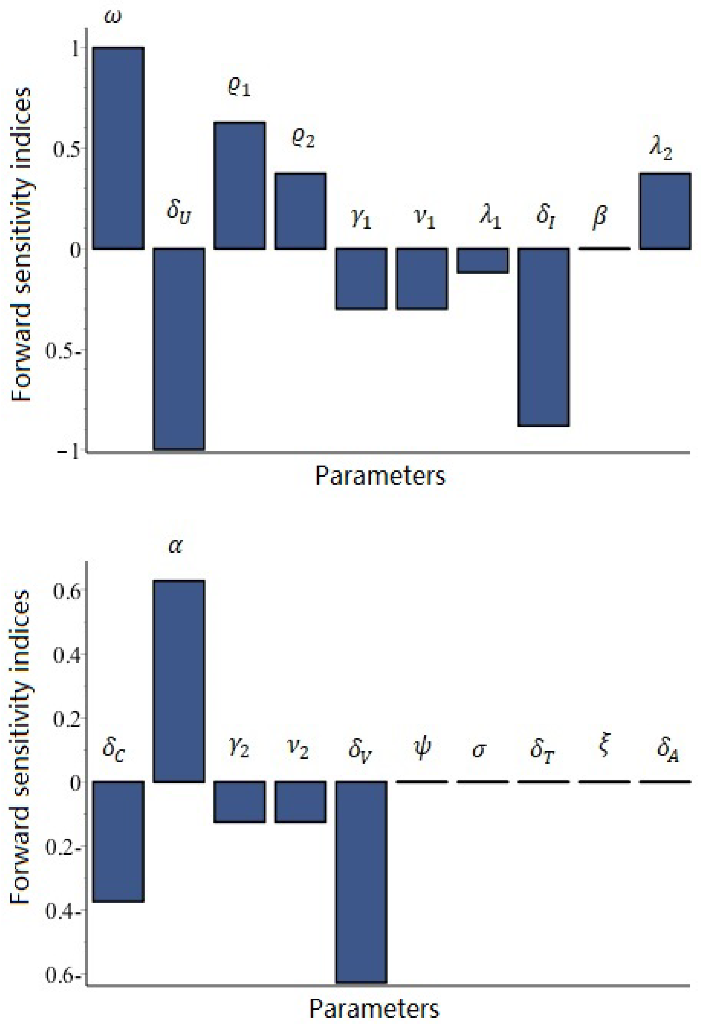
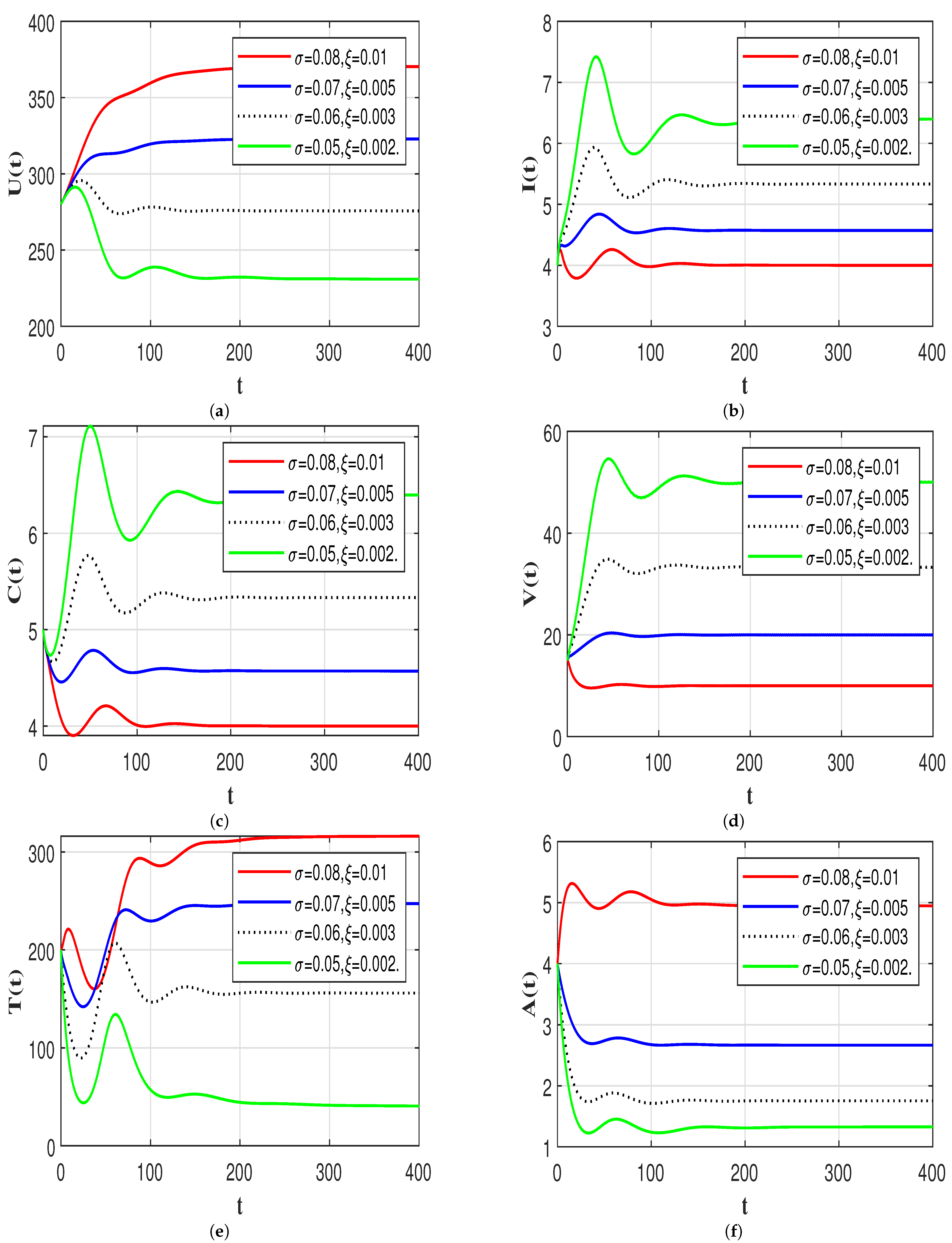
In this section, we ran numerical simulations for the models (9)–(14) using a specific form of the probability distribution function, such as:

$$F_i(\nu )=\varsigma (\nu -{\nu }_i),$$

where $\varsigma (.)$ is the Dirac delta function and ${\nu }_i\in \left[0,k_i\right],$ $i=1,2$ are constants. Let $k_i$ tend to ∞, then

$${\int }_0^{\infty }{F}_j(\theta )d\theta =1,{\mathcal{G}}_j={\int }_0^{\infty }\varsigma (\theta -{\nu }_j)e^{-{\gamma }_j\theta }d\theta =e^{-{\gamma }_j{\nu }_j},j=1,2.$$

Model (9)–(14) then becomes:

$$\begin{array}{cc}\frac{dU}{dt}\hfill & =\omega -{\delta }_{U}U-U\left({\varrho }_{1}V+{\varrho }_{2}C\right),\hfill \end{array}$$

(62)

$$\begin{array}{cc}\frac{dI}{dt}\hfill & =e^{-{\gamma }_1{\nu }_1}{U}_{{\nu }_1}\left({\varrho }_1{V}_{{\nu }_1}+{\varrho }_2{C}_{{\nu }_1}\right)-\left({\lambda }_1+{\delta }_I\right)I-\beta IT,\hfill \end{array}$$

(63)

$$\begin{array}{cc}\frac{dC}{dt}\hfill & ={\lambda }_{2}I-{\delta }_{C}C,\hfill \end{array}$$

(64)

$$\begin{array}{cc}\frac{dV}{dt}\hfill & =\alpha e^{-{\gamma }_2{\nu }_2}{I}_{{\nu }_2}-{\delta }_{V}V-\psi AV,\hfill \end{array}$$

(65)

$$\begin{array}{cc}\frac{dT}{dt}\hfill & =\sigma IT-{\delta }_{T}T,\hfill \end{array}$$

(66)

$$\begin{array}{cc}\frac{dA}{dt}\hfill & =\xi AV-{\delta }_{A}A.\hfill \end{array}$$

(67)

For this model, the threshold parameters become

$$\begin{array}{cc}{\Re }_0\hfill & =\frac{\omega e^{-{\gamma }_1{\nu }_1}\left({\varrho }_1{\delta }_C\alpha e^{-{\gamma }_2{\nu }_2}+{\varrho }_2{\lambda }_2{\delta }_V\right)}{{\delta }_U{\delta }_V{\delta }_C\left({\lambda }_1+{\delta }_I\right)},{\Re }_1=\frac{\sigma {\delta }_U{\delta }_V{\delta }_C\left({\Re }_0-1\right)}{{\delta }_T({\delta }_C{\varrho }_1\alpha e^{-{\gamma }_2{\nu }_2}+{\delta }_V{\lambda }_2{\varrho }_2)},\hfill \\ {\Re }_2\hfill & =\frac{{\delta }_C\alpha \xi e^{-{\gamma }_2{\nu }_2}{C}_3}{{\delta }_A{\delta }_V{\lambda }_2},{\Re }_3=\frac{{\delta }_T\xi \alpha e^{-{\gamma }_2{\nu }_2}}{{\delta }_V{\delta }_A\sigma },{\Re }_4=\frac{\sigma \omega e^{-{\gamma }_1{\nu }_1}\left({\delta }_C{\delta }_A{\varrho }_1\sigma +{\delta }_T{\varrho }_2\xi {\lambda }_2\right)}{{\delta }_T\left({\lambda }_1+{\delta }_I\right)\left({\delta }_U{\delta }_C\sigma \xi +{\delta }_C{\delta }_A{\varrho }_1\sigma +{\delta }_T{\varrho }_2\xi {\lambda }_2\right)}.\hfill \end{array}$$

We fixed the values of some parameters, which were taken from the literature (see

Table 2. Model parameters.

Parameter	Value	Source	Parameter	Value	Source	Parameter	Value	Source
$\omega$	10	[39,40,41]	$\beta$	$0.001$	[27]	$\psi$	$0.8$	[42]
${\delta }_U$	$0.01$	[40,43,44]	${\delta }_C$	$0.1$	[27]	${\delta }_T$	$0.32$	[27]
${\lambda }_1$	$0.1$	[27]	$\alpha$	13	[27]	${\delta }_A$	0.1	[42]
${\delta }_I$	$0.75$	[27]	${\delta }_V$	$0.3$	[32]	${\gamma }_1$	0.1	[45]
${\gamma }_2$	$0.1$	[46]	${\lambda }_2$	$0.1$	Assumed

). The others parameters were chosen just to perform the numerical simulation.

7.1. Sensitivity Analysis of ${\Re }_0$ to the Parameters for Model (62)–(67)

Sensitivity analysis holds a crucial position within the realm of dynamic systems research, particularly within the fields of ecology and epidemiology [47]. One pivotal aspect of this research entails scrutinizing the sensitivity of model parameters. This involves the calculation of specific sensitivity indices for each parameter, shedding light on their contributions to the dynamics of diseases. This section delves into the sensitivity analysis of various parameters concerning ${\Re }_0$. In order to execute a sensitivity analysis, we calculated the normalized forward sensitivity index of a variable using the following formula:

$$S{E}_{\mu }=\frac{\mu }{{\Re }_0}\frac{\partial {\Re }_0}{\partial \mu }.$$

(68)

This equation provides the sensitivity index of ${\Re }_0$ concerning the parameter $\mu$. In the context of forward sensitivity analysis, we explored how the alterations of these parameters influence the value of ${\Re }_0$. This analytical approach allowed us to assess the sensitivity of ${\Re }_0$ to adjustments in each parameter, offering valuable insights into their respective impacts on the system’s dynamics. When applying Relation (68) to all parameters of System (62)–(67), the following outcomes are apparent:

(i) 

The parameters with positive sensitivity indices include $\omega ,{\varrho }_1,{\varrho }_2,{\lambda }_2$, and $\alpha$, with

$$\begin{array}{cc}S{E}_{\omega }\hfill & =1,S{E}_{{\varrho }_1}=S{E}_{\alpha }=\frac{e^{-{\gamma }_2{\nu }_2}\alpha {\varrho }_1{\delta }_C}{e^{-{\gamma }_2{\nu }_2}\alpha {\varrho }_1{\delta }_C+{\lambda }_2{\varrho }_2{\delta }_V},\hfill \\ S{E}_{{\varrho }_2}\hfill & =S{E}_{{}_{{\lambda }_2}}=\frac{{\lambda }_2{\varrho }_2{\delta }_V}{e^{-{\gamma }_2{\nu }_2}\alpha {\varrho }_1{\delta }_C+{\lambda }_2{\varrho }_2{\delta }_V}.\hfill \end{array}$$

This implies that any increase or decrease in the values of those parameters directly influences ${\Re }_0$, leading to either an increase or a decrease in its value.

(ii) 

The parameters with negative sensitivity indices, signifying that an increase in their values leads to a decrease in ${\Re }_0$, include ${\delta }_U,{\gamma }_1,{\nu }_1,{\lambda }_1,{\delta }_I,{\delta }_C,{\gamma }_2,{\nu }_2,$ and ${\delta }_V$, as delineated below:

$$\begin{array}{cc}\hfill S{E}_{{\delta }_U}& =-1S{E}_{{\gamma }_1}=S{E}_{{\nu }_1}=-{\gamma }_1{\nu }_1,S{E}_{{\lambda }_1}=-\frac{{\lambda }_1}{{\lambda }_1+{\delta }_I}\hfill \\ \hfill S{E}_{{\delta }_I}& =-\frac{{\delta }_I}{{\lambda }_1+{\delta }_I},S{E}_{{\delta }_C}=-\frac{{\lambda }_2{\varrho }_2{\delta }_V}{e^{-{\gamma }_2{\nu }_2}\alpha {\varrho }_1{\delta }_C+{\lambda }_2{\varrho }_2{\delta }_V}\hfill \\ \hfill S{E}_{{\gamma }_2}& =S{E}_{{\nu }_2}=-\frac{{\gamma }_2{\delta }_C{\nu }_2{e}^{-{\gamma }_2{\nu }_2}\alpha {\varrho }_1}{e^{-{\gamma }_2{\nu }_2}\alpha {\varrho }_1{\delta }_C+{\lambda }_2{\varrho }_2{\delta }_V},S{E}_{{\delta }_V}=-\frac{e^{-{\gamma }_2{\nu }_2}\alpha {\varrho }_1{\delta }_C}{e^{-{\gamma }_2{\nu }_2}\alpha {\varrho }_1{\delta }_C+{\lambda }_2{\varrho }_2{\delta }_V}\hfill \end{array}$$

(iii) 

The parameters $\beta ,$$\psi ,\sigma ,{\delta }_T,\xi ,$ and ${\delta }_A$ have no impact on the value of ${\Re }_0$.

When selecting ${\nu }_1=3$, ${\nu }_2=2$, ${\varrho }_1=0.00018$, ${\varrho }_2=0.0038$, $\sigma =0.03$, and $\xi =0.0001$, the sensitivity indices for various model parameters, calculated using the formula (68), are visualized in Figure 1 and summarized in

Table 3. Sensitivity index of ${\Re }_0$.

Parameter	Sensitivity Index	Parameter	Sensitivity Index	Parameter	Sensitivity Index
$\omega$	1	${\delta }_I$	$-882\times {10}^{-3}$	${\delta }_V$	$-627\times {10}^{-3}$
${\delta }_U$	$-1$	$\beta$	0	$\psi$	0
${\varrho }_1$	$627\times {10}^{-3}$	${\lambda }_2$	$373\times {10}^{-3}$	$\sigma$	0
${\varrho }_2$	$373\times {10}^{-3}$	${\delta }_C$	$-373\times {10}^{-3}$	${\delta }_T$	0
${\gamma }_1$	$-0.3$	$\alpha$	$627\times {10}^{-3}$	$\xi$	0
${\nu }_1$	$-0.3$	${\gamma }_2$	$-125\times {10}^{-3}$	${\delta }_A$	0
${\lambda }_1$	$-118\times {10}^{-3}$	${\nu }_2$	$-125\times {10}^{-3}$

. Examining Table 3, we observe that a $10\%$ increase or decrease in the values of $\omega ,{\varrho }_1,{\varrho }_2,{\lambda }_2$, and $\alpha$ results in a corresponding $10\%$, 6.27%, 3.73%, 3.73%, and 6.269% increase or decrease in ${\Re }_0$, respectively. Conversely, a $10\%$ increase in the values of ${\delta }_U,{\gamma }_1,{\nu }_1,{\lambda }_1,{\delta }_I,{\delta }_C,{\gamma }_2,{\nu }_2,$ and ${\delta }_V$ leads to a reduction in ${\Re }_0$ by 10%, 3%, 3%, 1.18%, 8.82%, 3.73%, 1.25%, 1.25%, and 6.27%, respectively.

It is important to note that the correlation between time delay and ${\Re }_0$ is inverse, meaning that, as the time delay grows, ${\Re }_0$ typically decreases, indicating a decreased risk of infection. To recap, time delay is a pivotal factor in determining ${\Re }_0$’s value and, consequently, the generation of infected cells within epidemiological models. Extended time delays are connected to diminished ${\Re }_0$ values and a reduced number of infected cells, while shorter time delays are associated with elevated ${\Re }_0$ values and an increased count of infected cells. Grasping this connection is crucial for evaluating the likelihood of infection cases and formulating effective treatment strategies.

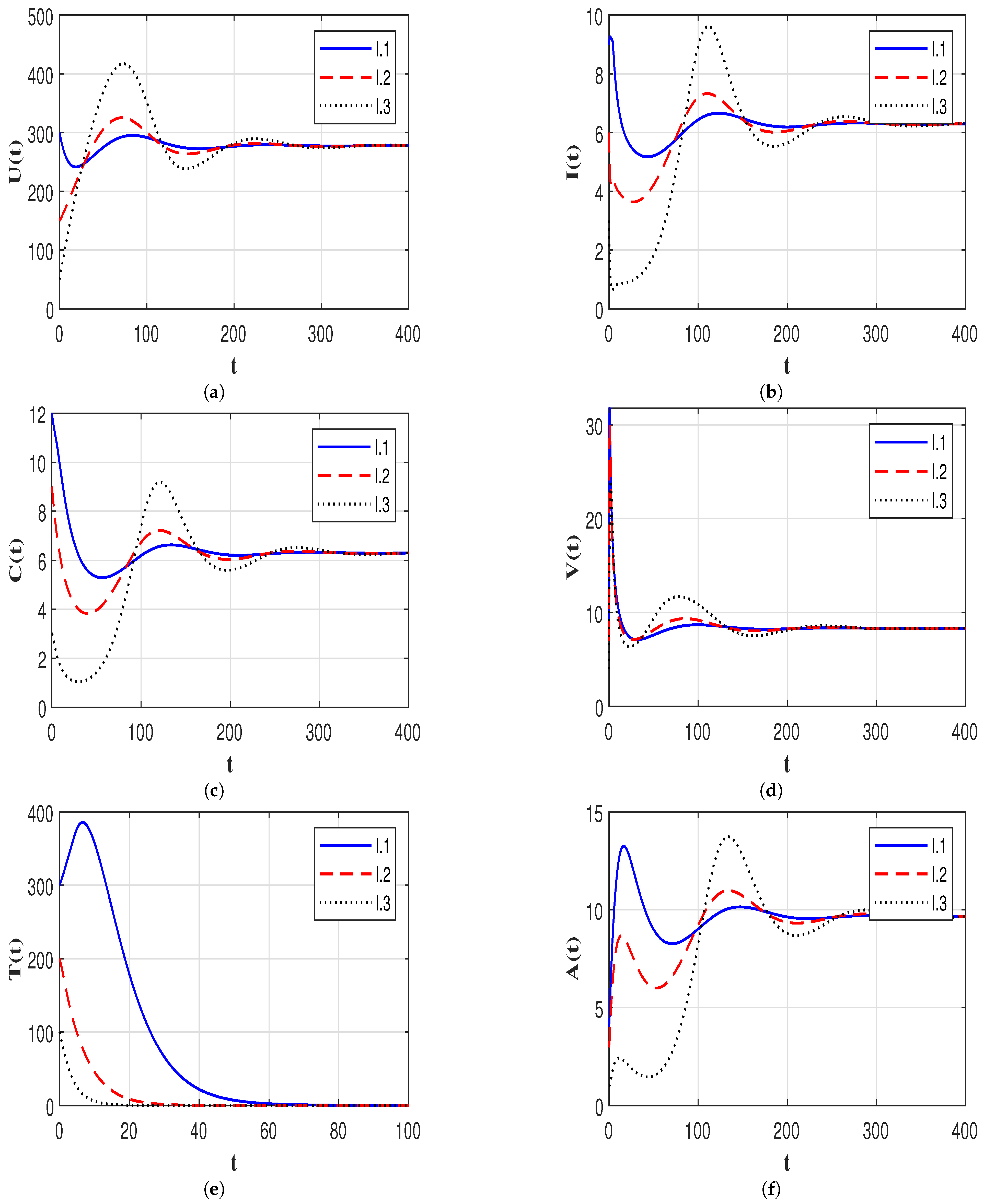
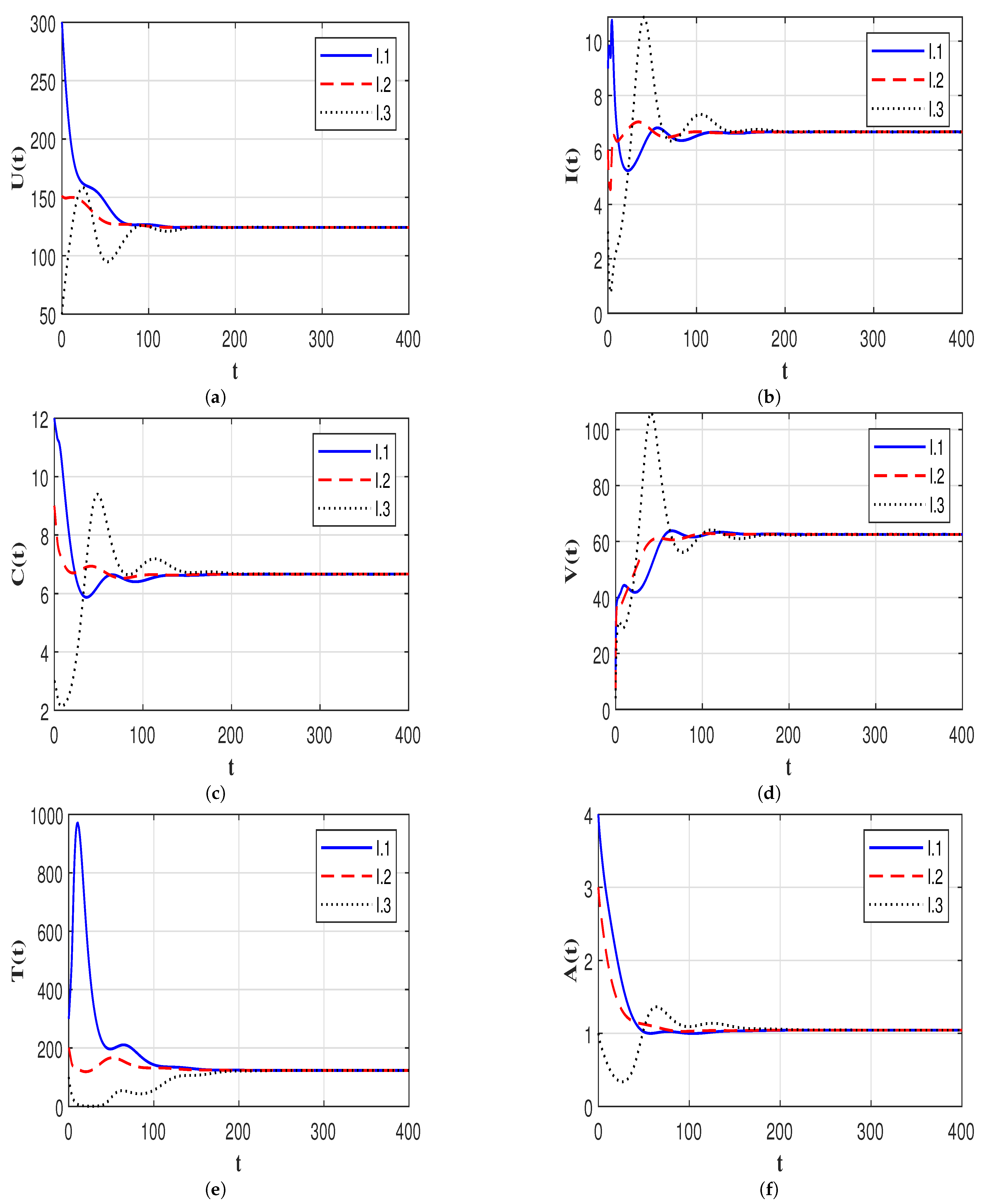
7.2. Stability of the Equilibria

In this subsection, we chose the delay parameters to be ${\nu }_1=3$ and ${\nu }_2=2$. We then used numerical simulation to illustrate our results given in Theorems 1–5. To obtain the numerical solutions of the model, we used the MATLAB’s dde23 solver. To illustrate the global stability, we chose three different initial conditions as:

I.1:  $(U(\theta ),I(\theta ),C(\theta ),V(\theta ),T(\theta ),A(\theta ))=(300,9,12,8,300,4);$

I.2:  $(U(\theta ),I(\theta ),C(\theta ),V(\theta ),T(\theta ),A(\theta ))=(150,6,9,7,200,3);$

I.3: $(U(\theta ),I(\theta ),C(\theta ),V(\theta ),T(\theta ),A(\theta ))=(50,3,3,4,100,1).$$\theta \in [-3,0]$.

We mention that, since we did not have real data, these initial values were chosen just for numerical purposes.

Under the preceding beginning conditions, selecting the chosen values of ${\varrho }_1,$ ${\varrho }_2,$ $\sigma$, and $\xi$ resulted in the following scenarios:

Scenario 1 (stability of $E{P}_0$): ${\varrho }_1=0.00001$, ${\varrho }_2=0.001$, $\sigma =0.001$, and $\xi =0.001$. These values give ${\Re }_0=0.39<1$. The numerical solutions eventually reach the equilibrium $E{P}_0=\left(1000,0,0,0,0,0\right)$ (see Figure 2). The numerical results shown in Figure 2 agree with the results of Theorem 1. This indicates that the HIV-1 particles ultimately are eradicated.

Scenario 2 (stability of $E{P}_1$): ${\varrho }_1=0.00018$, ${\varrho }_2=0.0038$, $\sigma =0.03$, and $\xi =0.0001$. These choices give ${\Re }_0=8.88>1$, ${\Re }_1=0.73<1$, and ${\Re }_2=0.29<1$ and create the persistent state of lacking immunity $E{P}_1=\left(112.64,7.73,7.73,274.38,0,0\right)$. Figure 3 illustrates the global stability of $E{P}_1$, which is proven in Theorem 2. This indicates that the levels of infected cells and viruses are small and insufficient to stimulate the adaptive immune response.

Scenario 3 (stability of $E{P}_2$): ${\varrho }_1=0.0001$, ${\varrho }_2=0.004$, $\sigma =0.048$, and $\xi =0.00039$. Using the data values in Table 2, we obtain ${\Re }_1=1.1086>1$ and ${\Re }_3=0.92<1$. The numerical simulations showed that $E{P}_2=\left(165.79,6.67,6.67,236.52,77.002,0\right)$ is G.A.S. (see Figure 4). This observation agrees with the outcomes of Theorem 3. This suggests that the CTL immune response is activated to remove infected cells without the need for antibodies.

Scenario 4 (stability of $E{P}_3$): ${\varrho }_1=0.0001$, ${\varrho }_2=0.004$, $\sigma =0.04$, and $\xi =0.012$. The values in Table 2 give ${\Re }_2=26.8028>1$ and ${\Re }_4=0.84<1$. The numerical solutions plotted in Figure 5 converge to $E{P}_3=\left(277.66,6.30,6.29,8.33,0,9.68\right)$. We see that, starting from any initial value, the concentration of the CTLs will go to zero, while all other compartments eventually tend to be constant over time. This supports the result of Theorem 4.

Scenario 5 (stability of $E{P}_4$): ${\varrho }_1=0.0007$, ${\varrho }_2=0.004$, $\sigma =0.048$, and $\xi =0.0016$. The values in Table 2 give ${\Re }_3=3.78>1$ and ${\Re }_4=1.14>1$. The numerical solutions displayed in Figure 6 tend to $E{P}_4=$$\left(124.35,6.67,6.67,62.5,123.04,1.04\right)$. We observed that, starting from any initial value, the concentrations of all compartments finally tend to be constant as time goes on. Consequently, $E{P}_4$ is G.A.S., and this agrees with the result of Theorem 5. This case represents the patient livedwith HIV-1 and that the adaptive immunity is active.

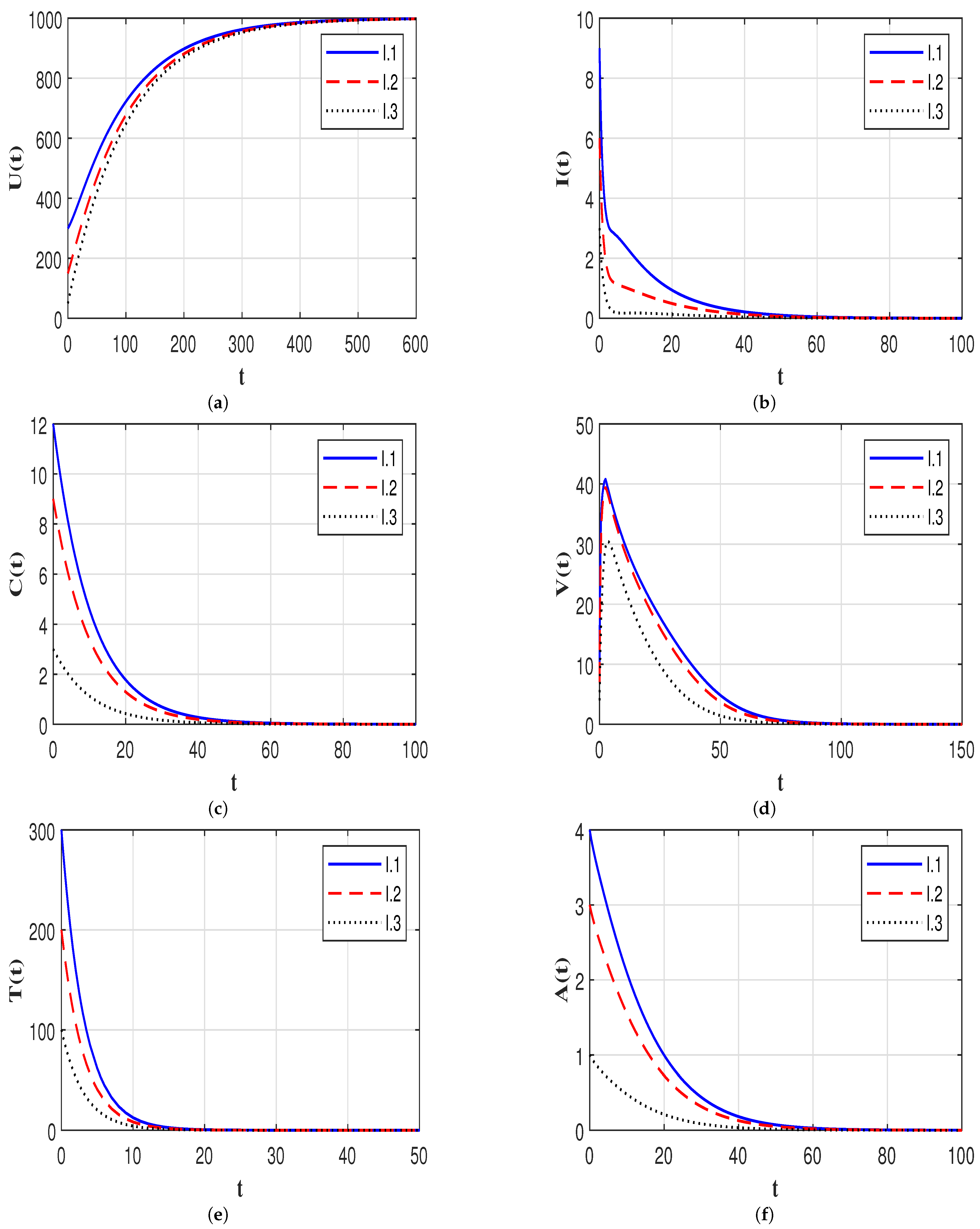
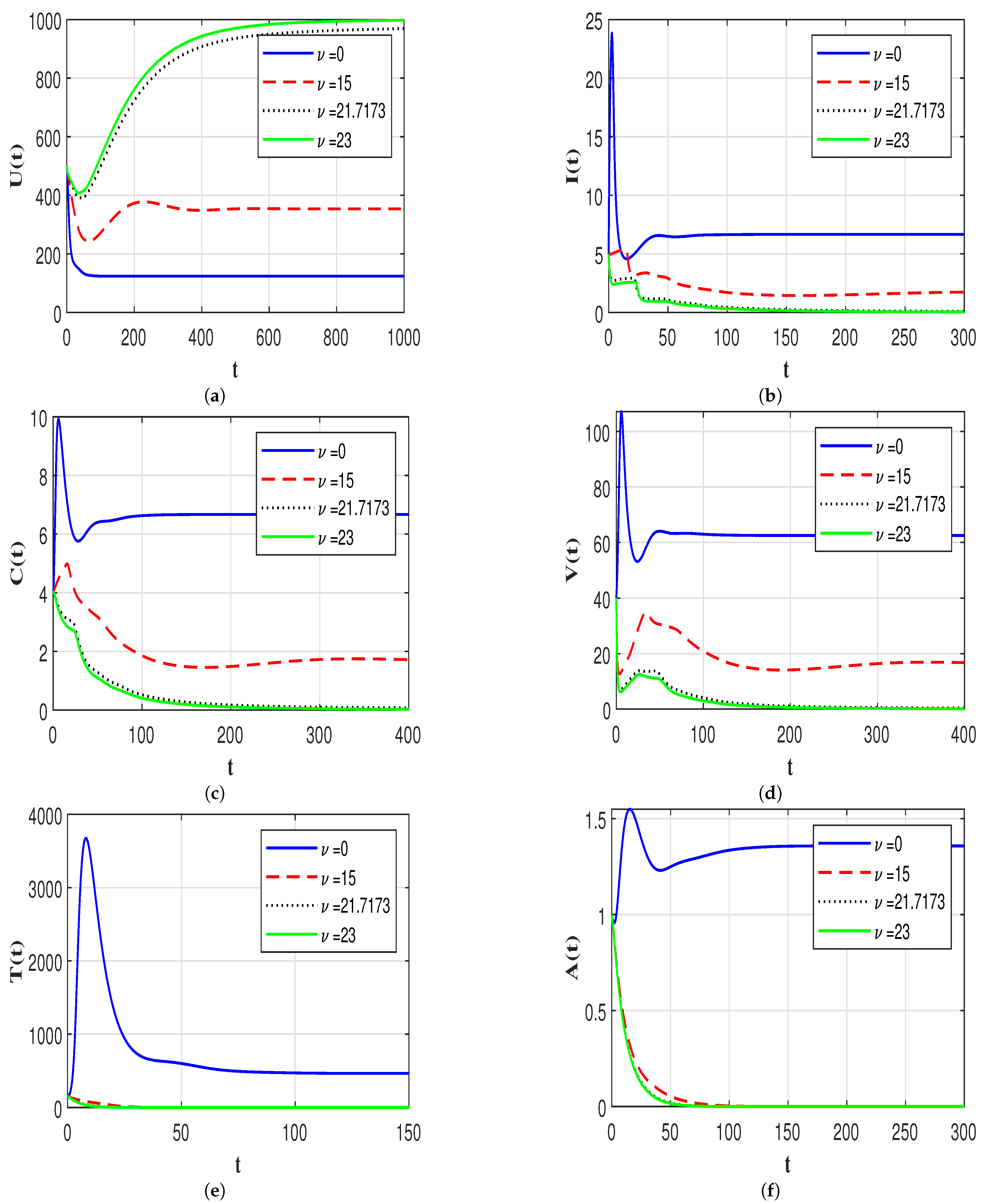
7.3. Effect of Time Delays on the HIV-1 Dynamics

In this part, we show the effect of time delay on the solutions of the system. We fixed the values ${\varrho }_1=0.0007$, ${\varrho }_2=0.004,$$\sigma =0.048$, and $\xi =0.0016$. Let us take $\nu ={\nu }_1={\nu }_2$, then the basic reproduction number ${\Re }_0$ becomes

$${\Re }_0=\frac{\omega e^{-{\gamma }_1\nu }\left({\varrho }_1{\delta }_C\alpha e^{-{\gamma }_2\nu }+{\varrho }_2{\lambda }_2{\delta }_V\right)}{{\delta }_U{\delta }_V{\delta }_C\left({\lambda }_1+{\delta }_I\right)}.$$

We observed that ${\Re }_0$ is a decreasing function of $\nu$. Therefore, the stability of the system we will change as $\nu$ changes. Since we are interested in the stabilization of the uninfected equilibrium $E{P}_0$, we computed the critical value of the delay ${\nu }_{cr}$, which makes

$${\Re }_0=\frac{\omega e^{-{\gamma }_1{\nu }_{cr}}\left({\varrho }_1{\delta }_C\alpha e^{-{\gamma }_2{\nu }_{cr}}+{\varrho }_2{\lambda }_2{\delta }_V\right)}{{\delta }_U{\delta }_V{\delta }_C\left({\lambda }_1+{\delta }_I\right)}=1.$$

(69)

By solving Equation (69) numerically, we obtain ${\nu }_{cr}=21.7173$. Then, we have that if $\nu \ge 21.7173$, then ${\Re }_0\le 1$ and $E{P}_0$ is G.A.S., and the virus will be eradicated. Now, we study the impact of delay parameter $\nu$ on the solutions of System (62)–(67) with initial values:

I.4: $(U(\theta ),I(\theta ),C(\theta ),V(\theta ),T(\theta ),A(\theta ))=(500,5,4,40,150,1),$ where $\theta \in [-max\{{\nu }_1,{\nu }_2\},0]$.

Figure 7 demonstrates the impact of $\nu$ on the system’s solutions. We observed that, as $\nu$ increases, the level of uninfected CD4${}^{+}$T cells will increase, while the levels of other compartments will decrease.

Biologically, time delays play important roles in HIV-1 progression, which gives some indications of how to control the infection. Sufficiently large time delays result in slower HIV-1 development, and HIV-1 is controlled and may disappear. This may give an indication of the possibility of creating new HIV-1 drugs that extend the delay time.

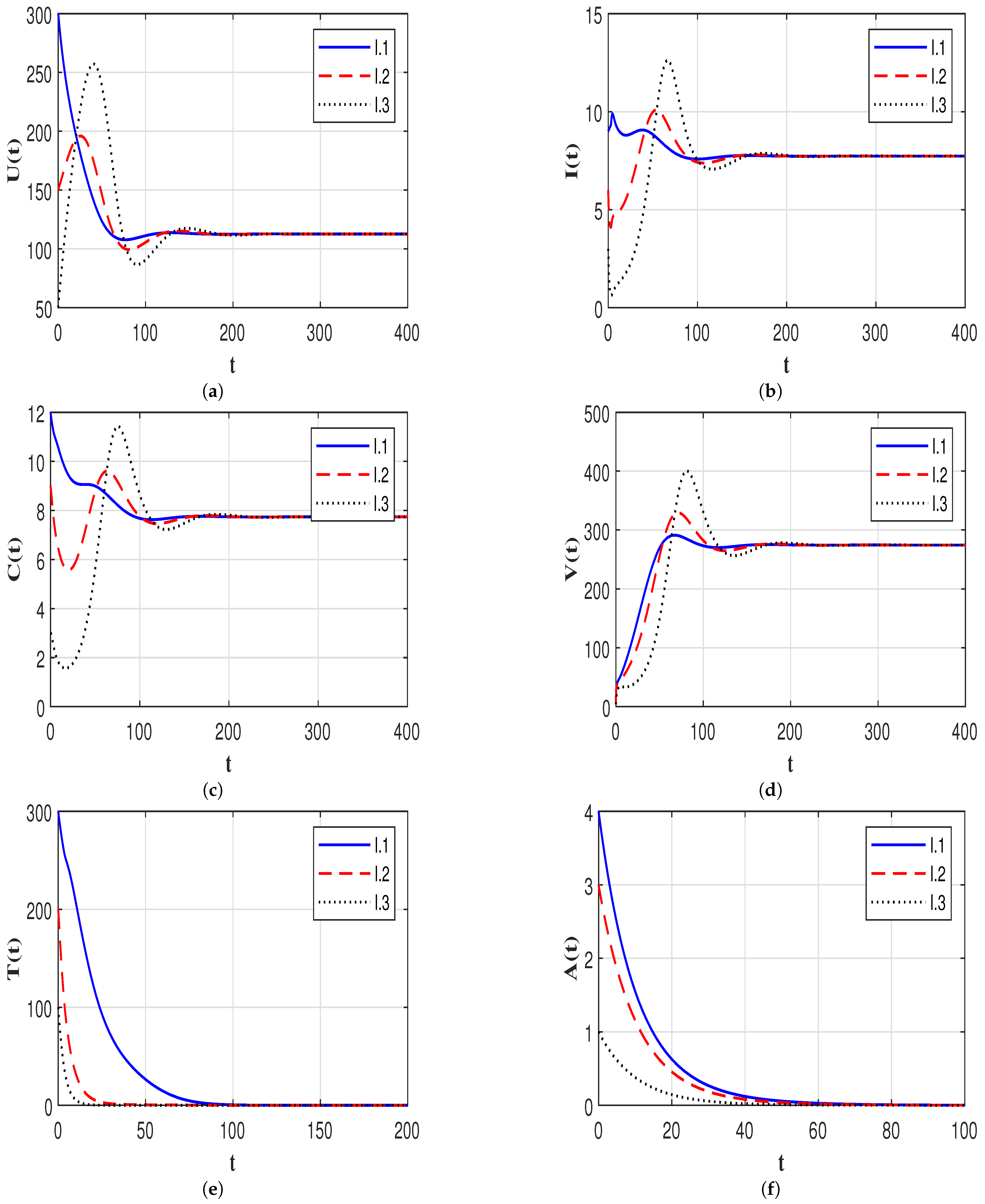
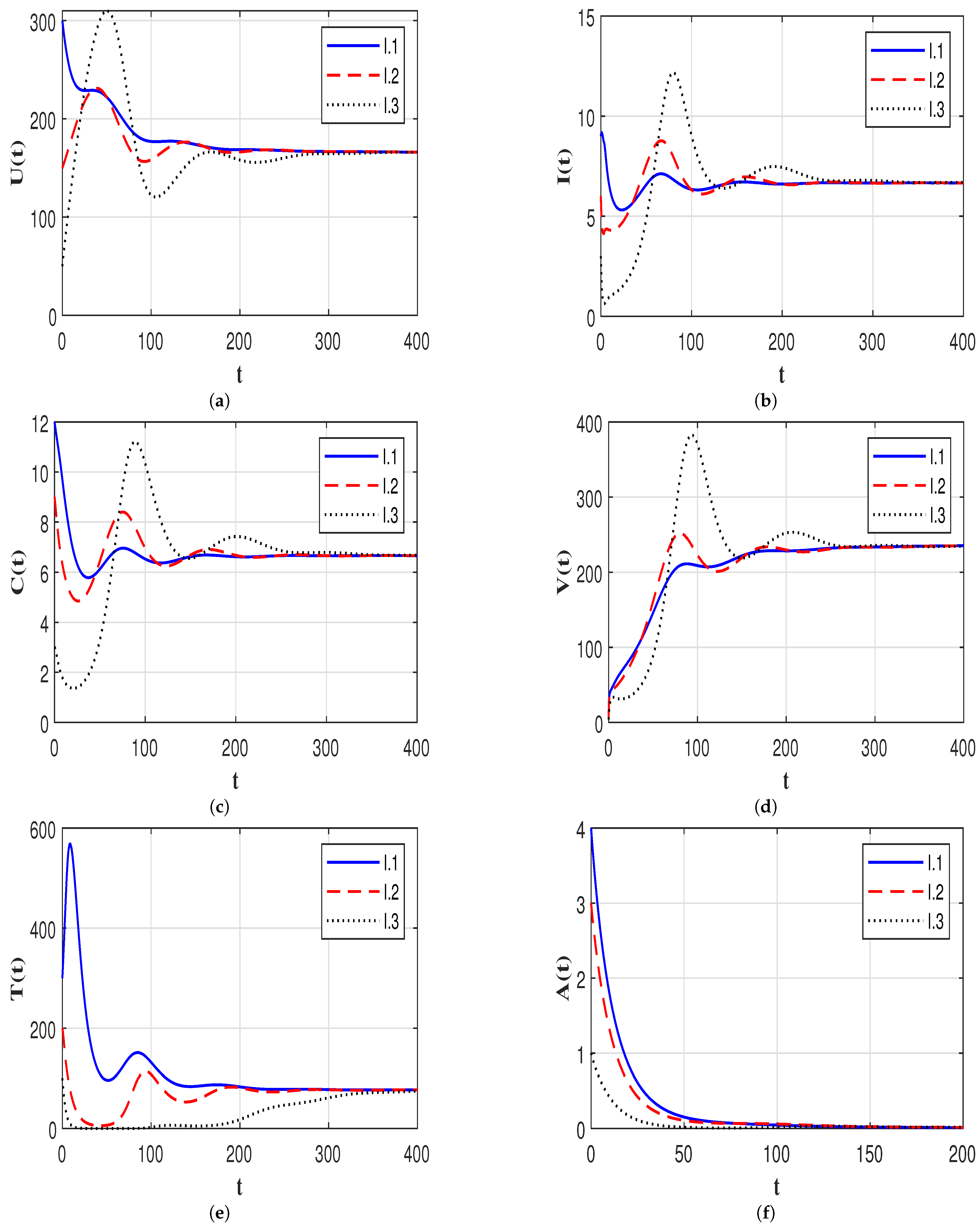
7.4. Effect of Immune Response on the HIV-1 Dynamics

In this part, we show the effect of immune response on the HIV-1 dynamics. We used the parameters given in Table 2 and fixed the parameters ${\varrho }_1=0.00018$, ${\varrho }_2=0.0038$, ${\nu }_1=3$, and ${\nu }_2=2$. We considered the following initial condition:

I.5: $(U(\theta ),I(\theta ),C(\theta ),V(\theta ),T(\theta ),A(\theta ))=(280,4,5,15,200,4),$ where $\theta \in [-3,0]$.

We varied the parameters $\sigma$ and $\xi$ as shown in Figure 8, which displays that, whenever the activity of the immune response changes, the dynamic behavior of the virus changes. We see that, when $\sigma$ and $\xi$ increase, the populations of uninfected CD4${}^{+}$T cell, CTLs, and antibodies increase, whereas the populations of infected cells, inflammatory cytokines, and free HIV-1 particles decrease.

8. Discussion

Recent research works have demonstrated that, during HIV-1 infection, pyroptosis is associated with the release of inflammatory cytokines. This can attract more CD4${}^{+}$T cells for infection and can lead to more CD4${}^{+}$T cell death. Understanding the dynamics of HIV-1 within the host under the influence of inflammatory cytokines is, thus, urgently needed. In this paper, we developed a cytokine-enhanced HIV-1 dynamics model with adaptive immunity and distributed delays. The model admits five equilibrium points as follows:

• The uninfected equilibrium, $E{P}_0$, usually exists, and it is G.A.S. when ${\Re }_0\le 1$. In this state, the number of HIV-1 particles eventually converges to 0. Different control plans can be applied to make

  $${\Re }_0=\frac{\omega e^{-{\gamma }_1{\nu }_1}}{{\delta }_U}\left[\frac{{\varrho }_1\alpha e^{-{\gamma }_2{\nu }_2}}{{\delta }_V\left({\lambda }_1+{\delta }_I\right)}+\frac{{\varrho }_2{\lambda }_2}{{\delta }_C\left({\lambda }_1+{\delta }_I\right)}\right]\le 1.$$
  These plans are, for example:

(i) Reducing both parameters ${\varrho }_1$ and ${\varrho }_2$. This may be achieved by applying two types of treatments: RTI [11] and necrosulfonamide [38], with drug efficacies ${ϵ}_1\in [0,1]$ and ${ϵ}_2\in [0,1]$, respectively. Thus, parameters ${\varrho }_1$ and ${\varrho }_2$ will be $(1-{ϵ}_1){\varrho }_1$ and $(1-{ϵ}_2){\varrho }_2$, respectively. We note that the basic reproduction number ${\widehat{\Re }}_0$ of a model that neglects the role of inflammatory cytokines might be underevaluated. Due to this, the treatment efficacy determined by this basic reproduction number is lower than what is necessary to eradicate the infection. We note also that ${\Re }_0$ does not depend on the humoral and CTL parameters. Therefore, humoral and CTL immunities play the role of controlling the HIV-1 infection, but not in clearing it. Our proposed model under the effect of anti-viral drugs can be considered as a nonlinear control system. Therefore, different control strategies can be applied for the stabilization of the system around a desired equilibrium (see, e.g., [48,49,50]).

(ii) Enlarging the length of delay periods ${\nu }_1$ and ${\nu }_2$ [35]. This may be performed if a new class of treatments is developed to prolong the delay periods and, then, inhibit HIV-1 progression.

• The chronic infection equilibrium with inactive immune response, $E{P}_1$, exists when ${\Re }_0>1$. Moreover, $E{P}_1$ is G.A.S. when ${\Re }_0>1$, ${\Re }_1\le 1$, and ${\Re }_2\le 1$. In this situation, HIV-1 is present, but without any immune response. This can happen when the populations of both HIV-1 and infected cells are insufficient to activate the immune system’s reaction, i.e., $V\le \frac{{\delta }_A}{\xi }$ and $I_4\le \frac{{\delta }_T}{\sigma }$.
• The chronic infection equilibrium with only CTL immunity, $E{P}_2$, exists when ${\Re }_1>1$. Further, $E{P}_2$ is G.A.S. when ${\Re }_1>1$ and ${\Re }_3\le 1$. In this case, HIV-1 exists in the body under CTL immune response only. This can happen when the number of viruses in the body becomes small and insufficient to activate the humoral immune response, i.e., $V\le \frac{{\delta }_A}{\xi }$.
• The chronic infection equilibrium with only humoral immunity, $E{P}_3$, exists when ${\Re }_2>1$. Further, $E{P}_3$ is G.A.S. when ${\Re }_2>1$ and ${\Re }_4\le 1$. In this case, HIV-1 exists in the body under humoral immune response only. This can happen when the number of infected cells becomes small and insufficient to activate the CTL immune response, i.e., $I_4\le \frac{{\delta }_T}{\sigma }$.
• The chronic infection equilibrium with both CTL and humoral immunities, $E{P}_4$, exists and is G.A.S. when ${\Re }_3>1$ and ${\Re }_4>1$. In this case, HIV-1 infection is chronic, where both humoral and CTL immune responses are activated.

The primary drawback of our study is that we were unable to estimate the values of the model’s parameters using real data. The reasons are as follows: (i) There is still a lack of real data on HIV-1 infection; (ii) it may not be very accurate to compare our results with a small number of real studies; (iii) it is difficult to gather real data from patients who are HIV-1 infected; (iv) conducting experiments to obtain real data is outside the purview of this paper. As a result, when real data become available, the theoretical conclusions reached in this study need to be compared against empirical findings.

9. Conclusions

In this paper, we formulated an HIV-1 model to obtain insight into the HIV-1 dynamics, taking the role of inflammatory cytokines into consideration. The effect of both humoral and CTL immunities on HIV-1 infection was included. Two distributed time delays were incorporated: (i) delay in the HIV-1 infection of uninfected CD4${}^{+}$T cells and (ii) delay in the maturation of recently released HIV-1 virions. We first showed the fundamental properties of the solutions, nonnegativity, and boundedness. Then, we established that the model admits five equilibria: $E{P}_i$, $i=0,1,\dots ,4$. We derived five threshold parameters, ${\Re }_i$, $i=0,1,\dots ,4,$ which completely determine the existence and global stability of the model’s equilibria. We used the Lyapunov method to prove the global asymptotic stability for all equilibria. We solved the model numerically and presented the results graphically. We found an agreement between the numerical and theoretical findings. A sensitivity analysis was performed to establish how the values of the model’s parameters affect the basic reproduction number ${\Re }_0$. We discussed the effect of pyroptosis, time delays, and adaptive immunity on the HIV-1 dynamics. We found that pyroptosis contributes to the number ${\Re }_0$, and then, neglecting it will make ${\Re }_0$ underevaluated. Besides the highly active antiretroviral drug therapies, which are usually used to inhibit viral replication, necrosulfonamide can be used to inhibit pyroptosis. Further, it was found that, increasing time delays can effectively decrease ${\Re }_0$ and, then, inhibit HIV-1 replication. This may indicate the development of new treatments that will prolong the delay. Furthermore, we showed that both humoral and CTL immunities have no effect on ${\Re }_0$, while this can result in less HIV-1 infection.

Our model can be extended by including (i) the mobility of cells and viruses [51], (ii) viral mutations [52], and (iii) stochastic interactions [53].

References

1. WHO. The Global Health Observatory. Available online: https://www.who.int/data/gho/data/themes/hiv-aids (accessed on 1 October 2023).
2. Wang, S.; Hottz, P.; Schechter, M.; Rong, L. Modeling the slow CD4+T cell decline in HIV-infected individuals. Plos Comput. Biol. 2015, 11, e1004665. [Google Scholar] [CrossRef] [PubMed]
3. Nowak, M.A.; Bangham, C.R.M. Population Dynamics of Immune Responses to Persistent Viruses. Science 1996, 272, 74–79. [Google Scholar] [CrossRef]
4. Wodarz, D.; May, R.M.; Nowak, M.A. The role of antigen-independent persistence of memory cytotoxic T lymphocytes. Int. Immunol. 2000, 12, 467–477. [Google Scholar] [CrossRef] [PubMed]
5. Wang, S.; Zou, D. Global stability of in host viral models with humoral immunity and intracellular delays. Appl. Math. Model. 2012, 36, 1313–1322. [Google Scholar] [CrossRef]
6. Tang, S.; Teng, Z.; Miao, H. Global dynamics of a reaction–diffusion virus infection model with humoral immunity and nonlinear incidence. Comput. Math. Appl. 2019, 78, 786–806. [Google Scholar] [CrossRef]
7. Zheng, T.; Luo, Y.; Teng, Z. Spatial dynamics of a viral infection model with immune response and nonlinear incidence. Z. Angew. Math. Phys. 2023, 74, 124. [Google Scholar] [CrossRef]
8. Kajiwara, T.; Sasaki, T.; Otani, Y. Global stability for an age-structured multistrain virus dynamics model with humoral immunity. J. Appl. Math. Comput. 2020, 62, 239–279. [Google Scholar] [CrossRef]
9. Dhar, M.; Samaddar, S.; Bhattacharya, P. Modeling the effect of non-cytolytic immune response on viral infection dynamics in the presence of humoral immunity. Nonlinear Dyn. 2019, 98, 637–655. [Google Scholar] [CrossRef]
10. Murase, A.; Sasaki, T.; Kajiwara, T. Stability analysis of pathogen-immune interaction dynamics. J. Math. Biol. 2005, 51, 247–267. [Google Scholar] [CrossRef]
11. Nowak, M.A.; May, R.M. Virus Dynamics; Oxford University Press: New York, NY, USA, 2000. [Google Scholar]
12. Lv, C.; Huang, L.; Yuan, Z. Global stability for an HIV-1 infection model with Beddington-DeAngelis incidence rate and CTL immune response. Commun. Nonlinear Sci. Numer. Simul. 2014, 19, 121–127. [Google Scholar] [CrossRef]
13. Jiang, C.; Kong, H.; Zhang, G.; Wang, K. Global properties of a virus dynamics model with self-proliferation of CTLs. Math. Appl. Sci. Eng. 2021, 2, 123–133. [Google Scholar] [CrossRef]
14. Ren, J.; Xu, R.; Li, L. Global stability of an HIV infection model with saturated CTL immune response and intracellular delay. Math. Biosci. Eng. 2020, 18, 57–68. [Google Scholar] [CrossRef] [PubMed]
15. Wang, A.P.; Li, M.Y. Viral dynamics of HIV-1 with CTL immune response. Discret. Contin. Dyn. Syst. Ser. 2021, 26, 2257–2272. [Google Scholar] [CrossRef]
16. Yang, Y.; Xu, R. Mathematical analysis of a delayed HIV infection model with saturated CTL immune response and immune impairment. J. Appl. Math. Comput. 2022, 68, 2365–2380. [Google Scholar] [CrossRef]
17. Chen, C.; Zhou, Y. Dynamic analysis of HIV model with a general incidence, CTLs immune response and intracellular delays. Math. Comput. Simul. 2023, 212, 159–181. [Google Scholar] [CrossRef]
18. Amarante-Mendes, G.P.; Adjemian, S.; Branco, L.M.; Zanetti, L.; Weinlich, R.; Bortoluci, K.R. Pattern recognition receptors and the host cell death molecular machinery. Front. Immunol. 2018, 9, 2379. [Google Scholar] [CrossRef]
19. Jiang, Y.; Zhang, T. Global stability of a cytokine-enhanced viral infection model with nonlinear incidence rate and time delays. Appl. Math. Lett. 2022, 132, 108110. [Google Scholar] [CrossRef]
20. Doitsh, G.; Galloway, N.L.K.; Geng, X.; Yang, Z.; Monroe, K.M.; Zepeda, O.; Hunt, P.W.; Hatano, H.; Sowinski, S.; Muñoz-Arias, I.; et al. Pyroptosis drives CD4 T-cell depletion in HIV-1 infection. Nature 2014, 505, 509–514. [Google Scholar] [CrossRef]
21. Wang, W.; Zhang, T. Caspase-1-mediated pyroptosis of the predominance for driving CD4+T cells death: A nonlocal spatial mathematical model. Bull. Math. Biol. 2018, 80, 540–582. [Google Scholar] [CrossRef]
22. Wang, W.; Feng, Z. Global dynamics of a diffusive viral infection model with spatial heterogeneity. Nonlinear Anal. Real World Appl. 2023, 72, 103763. [Google Scholar] [CrossRef]
23. Wang, W.; Ma, W.; Feng, Z. Complex dynamics of a time periodic nonlocal and time-delayed model of reaction-diffusion equations for modelling CD4+T cells decline. J. Comput. Appl. Math. 2020, 367, 112430. [Google Scholar] [CrossRef]
24. Wang, W.; Ren, X.; Ma, W.; Lai, X. New insights into pharmacologic inhibition of pyroptotic cell death by necrosulfonamide: A PDE model. Nonlinear Anal. Real World Appl. 2020, 56, 103173. [Google Scholar] [CrossRef]
25. Wang, W.; Ren, X.; Wang, X. Spatial-temporal dynamics of a novel PDE model: Applications to pharmacologic inhibition of pyroptosis by necrosulfonamide. Commun. Nonlinear Sci. Numer. Simul. 2021, 103, 106025. [Google Scholar] [CrossRef]
26. Xu, J. Dynamic analysis of a cytokine-enhanced viral infection model with infection age. Math. Biosci. Eng. 2023, 20, 8666–8684. [Google Scholar] [CrossRef] [PubMed]
27. Zhang, T.; Xu, X.; Wang, X. Dynamic analysis of a cytokine-enhanced viral infection model with time delays and CTL immune response. Chaos Solitons Fractals 2023, 170, 113357. [Google Scholar] [CrossRef]
28. Wodarz, D. Hepatitis C virus dynamics and pathology: The role of CTL and antibody responses. J. Gen. Virol. 2003, 84, 1743–1750. [Google Scholar] [CrossRef]
29. Wang, J.; Pang, J.; Kuniya, T.; Enatsu, Y. Global threshold dynamics in a five-dimensional virus model with cell-mediated, humoral immune responses and distributed delays. Appl. Math. Comput. 2014, 241, 298–316. [Google Scholar] [CrossRef]
30. Yan, Y.; Wang, W. Global stability of a five-dimensional model with immune responses and delay. Discret. Contin. Dyn. Syst. Ser. B 2012, 17, 401–416. [Google Scholar] [CrossRef]
31. Dubey, P.; Dubey, U.S.; Dubey, B. Modeling the role of acquired immune response and antiretroviral therapy in the dynamics of HIV infection. Math. Comput. Simul. 2018, 144, 120–137. [Google Scholar] [CrossRef]
32. Junxian, Y.; Wang, L. Dynamics analysis of a delayed HIV infection model with CTL immune response and antibody immune response. Acta Math. Sci. 2021, 41, 991–1016. [Google Scholar]
33. Kuang, Y. Delay Differential Equations with Applications in Population Dynamics; Academic Press: Boston, MA, USA, 1993. [Google Scholar]
34. Korobeinikov, A. Global properties of basic virus dynamics models. Bull. Math. Biol. 2004, 66, 879–883. [Google Scholar] [CrossRef]
35. Huang, G.; Takeuchi, Y.; Ma, W. Lyapunov functionals for delay differential equations model of viral infections. Siam J. Appl. Math. 2010, 70, 2693–2708. [Google Scholar] [CrossRef]
36. Hale, J.K.; Lunel, S.M.V. Introduction to Functional Differential Equations; Springer: New York, NY, USA, 1993. [Google Scholar]
37. Khalil, H.K. Nonlinear Systems, 3rd ed.; Prentice Hall: Upper Saddle River, NJ, USA, 2002. [Google Scholar]
38. Rathkey, J.K.; Zhao, J.; Liu, Z.; Chen, Y.; Yang, J.; Kondolf, H.C.; Benson, B.L.; Chirieleison, S.M.; Huang, A.Y.; Dubyak, G.R.; et al. Chemical disruption of the pyroptotic pore-forming protein gasdermin D inhibits inflammatory cell death and sepsis. Sci. Immunol. 2018, 3, eaat2738. [Google Scholar] [CrossRef]
39. Li, F.; Ma, W. Dynamics analysis of an HTLV-1 infection model with mitotic division of actively infected cells and delayed CTL immune response. Math. Methods Appl. Sci. 2018, 41, 3000–3017. [Google Scholar] [CrossRef]
40. Elaiw, A.M.; AlShamrani, N.H. Modeling and analysis of a within-host HTLV-I/HIV co-infection. Bol. Soc. Math. Mex. 2021, 1, 27–38. [Google Scholar] [CrossRef]
41. Perelson, A.S.; Kirschner, D.E.; de Boer, R. Dynamics of HIV Infection of CD4+T cells. Math. Biosci. 1993, 114, 81–125. [Google Scholar] [CrossRef]
42. Alshaikh; AlShamrani, N.H.; Elaiw, A.M. Stability of HIV/HTLV co-infection model with effective HIV-specific antibody immune response. Results Phys. 2021, 27, 104448. [Google Scholar] [CrossRef]
43. Callaway, D.S.; Perelson, A.S. HIV-1 infection and low steady state viral loads. Bull. Math. Biol. 2002, 64, 29–64. [Google Scholar] [CrossRef]
44. Mohri, H.; Bonhoeffer, S.; Monard, S.; Perelson, A.S.; Ho, D. Rapid turnover of T lymphocytes in SIV-infected rhesus macaques. Science 1998, 279, 1223–1227. [Google Scholar] [CrossRef]
45. Elaiw, A.M.; AlShamrani, N.H. Stability of a delayed adaptive immunity HIV infection model with sitrnt infected cells and cellular infection. J. Appl. Anal. Comput. 2021, 11, 964–1005. [Google Scholar]
46. Elaiw, A.M.; AlShamrani, N.H.; Hobiny, A.D. Stability of an adaptive immunity delayed HIV infection model with active and silent cell-to-cell spread. Math. Biosci. Eng. 2020, 17, 6401–6458. [Google Scholar] [CrossRef]
47. Marino, S.; Hogue, I.B.; Ray, C.J.; Kirschner, D.E. A methodology for performing global uncertainty and sensitivity analysis in systems biology. J. Theor. Biol. 2008, 254, 178–196. [Google Scholar] [CrossRef] [PubMed]
48. Chen, J.; Zhang, H.; Yin, G. Distributed dynamic event-triggered secure model predictive control of vehicle platoon against DoS attacks. IEEE Trans. Veh. Technol. 2022, 72, 2863–2877. [Google Scholar] [CrossRef]
49. Zhang, H.; Shi, Y.; Wang, J.; Chen, H. A new delay-compensation scheme for networked control systems in controller area networks. IEEE Trans. Ind. Electron. 2018, 65, 7239–7247. [Google Scholar] [CrossRef]
50. Elaiw, A.M.; Xia, X. HIV dynamics: Analysis and robust multirate MPC-based treatment schedules. J. Math. Appl. 2009, 359, 285–301. [Google Scholar] [CrossRef]
51. Elaiw, A.M.; AlAgha, A.D. Analysis of a delayed and diffusive oncolytic M1 virotherapy model with immune response. Nonlinear Anal. Real World Appl. 2020, 55, 103116. [Google Scholar] [CrossRef]
52. Bellomo, N.; Burini, D.; Outada, N. Multiscale models of Covid-19 with mutations and variants. Netw. Heterog. Media 2022, 17, 293–310. [Google Scholar] [CrossRef]
53. Gibelli, L.; Elaiw, A.M.; Alghamdi, M.A.; Althiabi, A.M. Heterogeneous population dynamics of active particles: Progression, mutations, and selection dynamics. Math. Model. Methods Appl. Sci. 2017, 27, 617–640. [Google Scholar] [CrossRef]
Figure 1. Forward sensitivity analysis to assess the influence of the system’s (62)–(67) parameters on 0 .
Computation 11 00217 g001
Figure 2. The equilibrium point E P 0 = 1000 , 0 , 0 , 0 , 0 , 0 is G.A.S. whenever 0 1 . (a) Uninfected CD4 + T cells; (b) infected CD4 + T cells; (c) inflammatory cytokines; (d) free HIV-1; (e) CTLs; (f) antibodies.
Computation 11 00217 g002
Figure 3. The equilibrium point E P 1 = 112.64 , 7.73 , 7.73 , 274.39 , 0 , 0 is G.A.S. whenever 0 > 1 , 1 1 and 2 1 . (a) Uninfected CD4 + T cells; (b) infected CD4 + T cells; (c) inflammatory cytokines; (d) free HIV-1; (e) CTLs; (f) antibodies.
Computation 11 00217 g003
Figure 4. The equilibrium point E P 2 = 165.78 , 6.66 , 6.66 , 236.51 , 77.003 , 0 is G.A.S. whenever 2 > 1 and 3 1 . (a) Uninfected CD4 + T cells; (b) infected CD4 + T cells; (c) inflammatory cytokines; (d) free HIV-1; (e) CTLs; (f) antibodies.
Computation 11 00217 g004
Figure 5. The equilibrium point E P 3 = 277.65 , 6.29 , 6.29 , 8.34 , 0 , 9.67 is G.A.S. whenever 3 > 1 and 4 1 . (a) Uninfected CD4 + T cells; (b) infected CD4 + T cells; (c) inflammatory cytokines; (d) free HIV-1; (e) CTLs; (f) antibodies.
Computation 11 00217 g005
Figure 6. The equilibrium point E P 4 = 124.35 , 6.66 , 6.66 , 62.5 , 123.04 , 1.0441 is G.A.S. whenever 3 > 1 and 4 > 1 . (a) Uninfected CD4 + T cells; (b) infected CD4 + T cells; (c) inflammatory cytokines; (d) free HIV-1; (e) CTLs; (f) antibodies.
Computation 11 00217 g006
Figure 7. Influence of the delay parameter ν on the solutions of System (62)–(67). (a) Uninfected CD4 + T cells; (b) infected CD4 + T cells; (c) inflammatory cytokines; (d) free HIV-1; (e) CTLs; (f) antibodies.
Computation 11 00217 g007
Figure 8. Influence of the immune response parameters σ and ξ on the solutions of System (62)–(67). (a) Uninfected CD4 + T cells; (b) infected CD4 + T cells; (c) inflammatory cytokines; (d) free HIV-1; (e) CTLs; (f) antibodies.
Computation 11 00217 g008