1. Introduction
Welding is often used to connect metallic structures [
1,
2,
3], including connecting metallic parts for oil and gas pipelines and other civil structures [
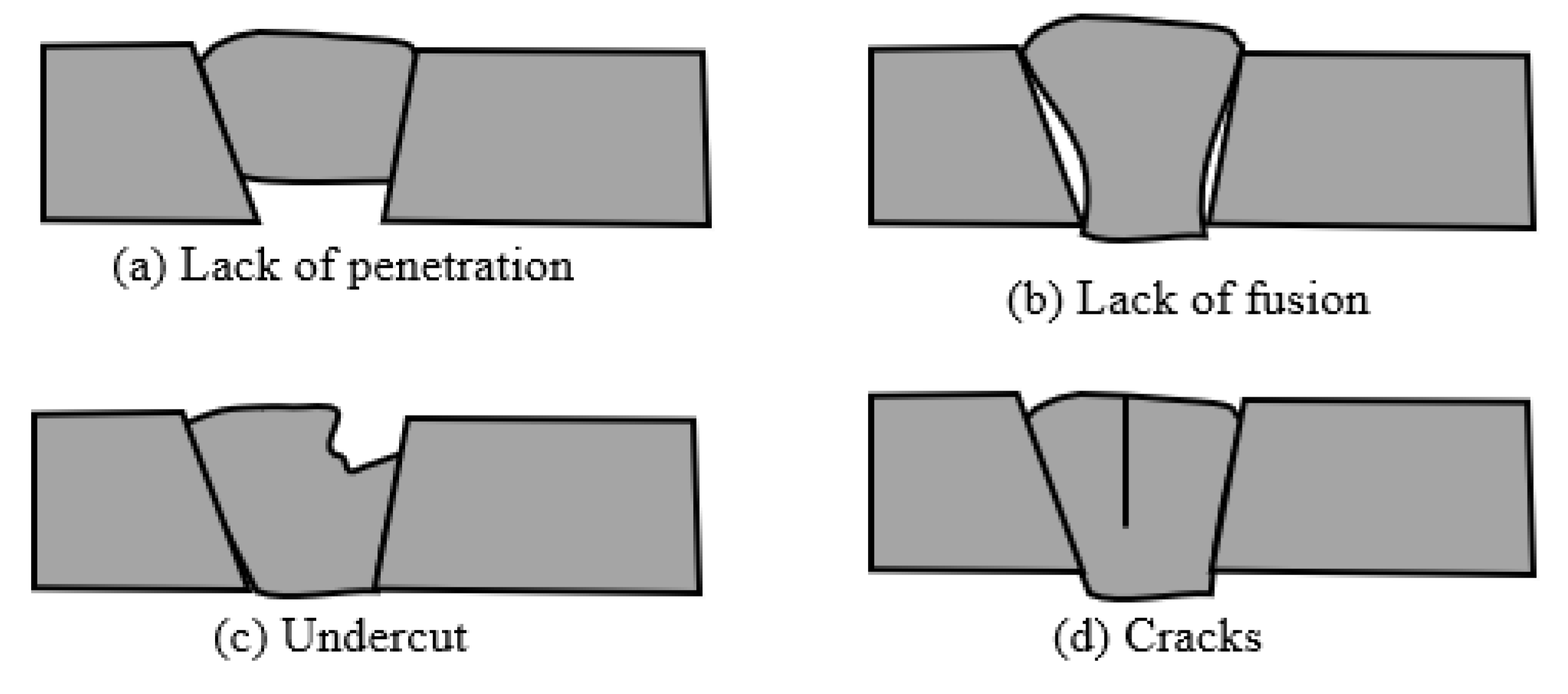
4]. Different forms of welding faults, including partial penetration, lack of fusion, cracking, and undercut are frequently observed due to the complicated properties of the welding procedure used in shops and on building sites [
4]. As a result, even seemingly minor welding errors frequently lead to early-age damage in materials and structures, such as corrosion caused by cracks [
4,
5,
6]. Thus, it is essential to inspect the weldment for structural health monitoring (SHM) [
7,
8,
9] during fabrication, construction, and afterward during the in-service phase to ensure welding quality [
10,
11,
12,
13,
14,
15].
Nondestructive testing methods, including ultrasonic, dye penetration, magnetic particle, and eddy current are widely used in pipeline damage detection [
16,
17,
18]. But for online testing, dye penetrant and magnetic particle testing typically necessitate removing the tested portion [
16]. Eddy current testing cannot be used on non-standard surfaces [
16]. However, ultrasonic-guided wave testing [
4,
19,
20] can be used to carry out large-scale and quantitative damage detection because of its benefits of non-contact, a large working area, and high sensitivity [
16,
21,
22].
Table 1 compares ultrasonic-guided wave testing with other non-destructive testing techniques for detecting pipe welding defects.
Weldment is a part of pipelines and is vulnerable to damage [
23,
24,
25,
26]. Rattanawangcharoen et al. [
27] used the finite element approach and wave expansion function to simulate the propagation of ultrasonic-guided waves with various weld shapes in thin-walled cylinders and studied the dispersion of axisymmetric guided waves in the area where the cylinders’ bonding materials were located. The resonance peak of the reflection coefficient was more pronounced as the joint thickness increased. The proposed method could be used to evaluate weld faults quantitatively and without causing any damage. Zhuang et al. [
28] also simulated the propagation of a symmetrical guided wave mode in welded steel pipes based on finite element analysis and analyzed the difference between weld joints with and without faults in the reflection coefficient.
Deep learning approaches have demonstrated their robustness in the signal processing of ultrasonic-guided waves [
29,
30,
31,
32]. CNN is one of the representative deep learning algorithms and it has the properties of local perception and parameter sharing, which enables CNN to efficiently learn the associated features from many samples [
16,
33]. Xu et al. [
34] used features extracted from the guided wave on several monitoring paths to train CNN and determined the length of the fatigue fracture. Su et al. [
35] established a damage classification model based on CNN. Frequency-domain characteristics of the ultrasonic-guided wave were used to train the model. Feng et al. [
36] developed a CNN model to detect damage based on image detection. Kumaresan et al. [
37] used CNN for transfer learning to classify welding defects. But, the CNN model did not consider the temporal connection of the collected signals. LSTM networks, a subset of Recurrent Neural Networks (RNNs), are renowned for their prowess in time series analysis, adept at capturing intricate temporal patterns. They have excelled in multiple fields: financial markets [
38,
39], forecasting stock prices [
40], healthcare, predicting patient outcomes from health records [
41], and natural language processing [
42]. LSTM’s adaptability and ability to tackle sequential data make them indispensable in a broad range of domains. LSTM has also been used to identify the damage information in the vibration signal damage because it can maintain the temporal correlation of vibration signals [
16]. Zhao et al. [
43] proposed the CNN and LSTM networks to achieve early damage detection and identify the cantilever beam breathing crack. Choe et al. [
44] used gated recurrent unit neural networks with LSTM to identify damage related to structures, which resulted in high damage identification performance. The time series features obtained by LSTM can be used to improve the damage detection accuracy, as demonstrated by the literature mentioned above.
In this study, the CNN-LSTM network was used to detect pipeline damage with different types of welding defects in a notch. Firstly, twenty-nine feature parameters were calculated and compared based on the training performance of different deep learning models, including CNN, LSTM, and CNN-LSTM models. The CNN-LSTM hybrid model was expected to achieve the highest performance because of its complex structure. It combined CNN and LSTM networks; as a result, it could help the hybrid network to extract temporal information comprehensively, which reduces the side effects of the CNN network. The LSTN network is followed the CNN network; the compressed information from the CNN network could be input into the LSTM network directly, and it could improve the training efficiency of the CNN-LSTM hybrid model. Furthermore, noise interference, different types of defects, and different types of pipeline embedment were designed to verify the effectiveness of the CNN-LSTM hybrid model.
2. Deep Learning Enriched Automation in Damage Detection
The structure of methodologies is shown in
Figure 1, including feature extraction, model training and testing, and classification. Different types of features were chosen, calculated, and trained by deep learning models. The most effective features were selected to express the signals’ information. Three deep learning approaches, including CNN, LSTM, and CNN-LSTM models, were then used to perform the data classification for detecting welding defects (type and severity). Noises were introduced to the original signals to discuss the robustness of the deep learning approaches.
2.1. CNN Model
CNN is a widely accepted deep learning approach with a deep neural network, consisting of convolutional, pooling, and a fully linked layer with a rectified linear activation function (ReLU), for data processing [
45,
46]. In this study, a one-dimensional (1D) signal was used as an input for the CNN network. The input data of the 1D signal vector is represented by
where
stands for features (i.e., time series signal data) and C stands for a class label. From a collection of features
, the following new feature map
is created [
45].
where a feature map
. The kernel
is applied to each array of features
within the input data specified as
, and
signifies a bias term [
45].
The average pooling layer receives the output of the convolutional layer and down samples the data [
47], which employs the ReLU activation function applying
to each input to the ReLU represented by x [
45]. Here, each feature map is subjected to the average-pooling process using the formula
, which yields the most important features [
45]. The fully connected layer, which contains the
function and provides the probability distribution across each class, receives these chosen features as input [
45]. As a result, the CNN network’s fully connected layer (FC) calculates the classes that make up its final output [
45].
2.2. LSTM Model
LSTM was developed to overcome recurrent neural networks (RNNs) with consideration of long-term memory of time-dependent information [
45]. This implies LSTMs possess the capacity to retain and establish connections between preceding data—often considerably distant in time from the current moment—to the present context [
45]. With the progression of LSTM research, enhancements such as the introduction of forget gates and peephole connections became integrated into the LSTM network [
45]. The forget gate replaces the constant error carousel (CEC) and aids in forgetting or resetting the states of memory cells [
45].
The functioning of the LSTM is as described below. The LSTM architecture receives an input sequence of data with length
that can be any length [
45]. Within the recurrent concealed stratum of the LSTM framework, the resultant sequence
is computed in an iterative manner, progressing from t = 1 to T. This is achieved through consistent write, read, and reset actions executed via the memory cell (me) of the input gate (
), forget gate (
), and output gate (
) [
45,
48]. The operation sequence at the time t can be described as follows [
45].
The forget gate is essential for removing self-recurrent values no longer useful and maintaining them for the next time step by multiplying them with the memory cell. Additionally, peephole connections allow each gate and memory cell to determine the exact timings of their outputs [
45]. This comprehensive LSTM architecture, with the forget gate and peephole connections, enhances the model’s ability to capture and utilize long-term dependencies in time series data.
2.3. CNN-LSTM Hybrid Model
A CNN-LSTM model was developed, as shown in
Figure 2. The proposed CNN-LSTM model used the convolution1D and average pooling1D layers to extract features from a number of variables affecting the categorization of defect types and to reduce the data distribution [
49,
50]. The following LSTM layer receives input from the average pooling1D layer’s output.
The original input vector of the CNN network, along with its corresponding class label, is denoted as . The resulting output of the CNN network, represented by , serves as the input for the subsequent LSTM network. In order to learn the long-range temporal relationships, the LSTM is fed with the feature vector created by the average pooling procedure in CNN.
In the context of detecting pipeline damage with various welding defects, the CNN-LSTM network serves as a powerful tool, offering efficient temporal feature extraction. In this study, a comprehensive analysis of deep learning models, including CNN, LSTM, and the CNN-LSTM hybrid, was conducted to determine the most suitable approach.
Table 2 illustrates and compares the structure of CNN, LSTM and CNN-LSTM networks. In our MATLAB training process, the learning rate is set to 0.1, the mini-batch size is set to 16, and the number of LSTM units is 100. The chosen activation functions are ReLU for the CNN layers and hyperbolic tangent (tanh) for the LSTM layers.
The CNN-LSTM hybrid model was expected to outperform others due to its intricate structure. This model combines the strengths of both CNN and LSTM networks, resulting in the comprehensive extraction of temporal information. In the CNN, LSTM, and CNN-LSTM models, we included batch normalization layers to standardize the outputs of each layer. This was done to reduce the chances of overfitting and enhance the robustness of the optimization process. The effectiveness of batch normalization layers has been supported by prior research [
51]. By integrating CNN before LSTM, the hybrid network can efficiently process spatial and sequential data. It captures essential spatial features via CNN and subsequently feeds this compressed information into LSTM for in-depth temporal analysis. This not only optimizes feature extraction but also reduces the potential side effects associated with using CNN in isolation.
The CNN-LSTM model was then put to the test under challenging conditions, including noise interference, various defect types, and distinct pipeline embedment scenarios. Its effectiveness in handling these complex and real-world situations was assessed. The combination of CNN and LSTM, offering a balance between spatial and temporal feature extraction, demonstrated its capability to robustly detect pipeline damage and welding defects in notches, making it a promising approach for real-world applications.
2.4. Features Extraction
Definition of Features
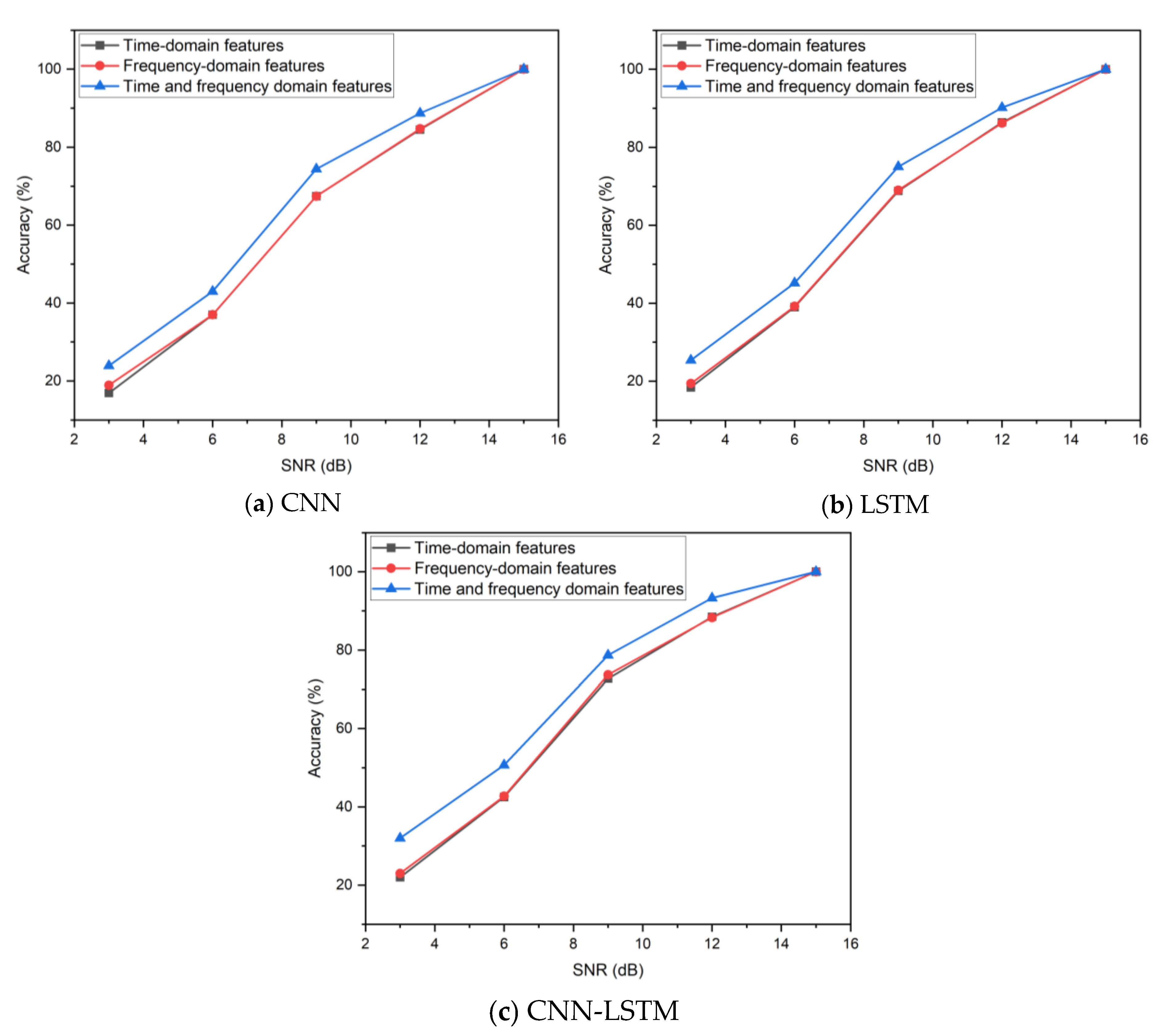
To define the fault characteristics in various types of damaged pipelines, 29 time- and frequency-domain feature parameters, comprising a total of 16 feature parameters in the time domain and 13 feature parameters in the frequency-domain, were chosen for this work. The detailed information is shown in
Table 3. These parameters were chosen in accordance with the findings of Chen’s study [
52]. In this study, feature extraction was used as a signal preprocessing method.
2.5. Evaluation of Model Performances
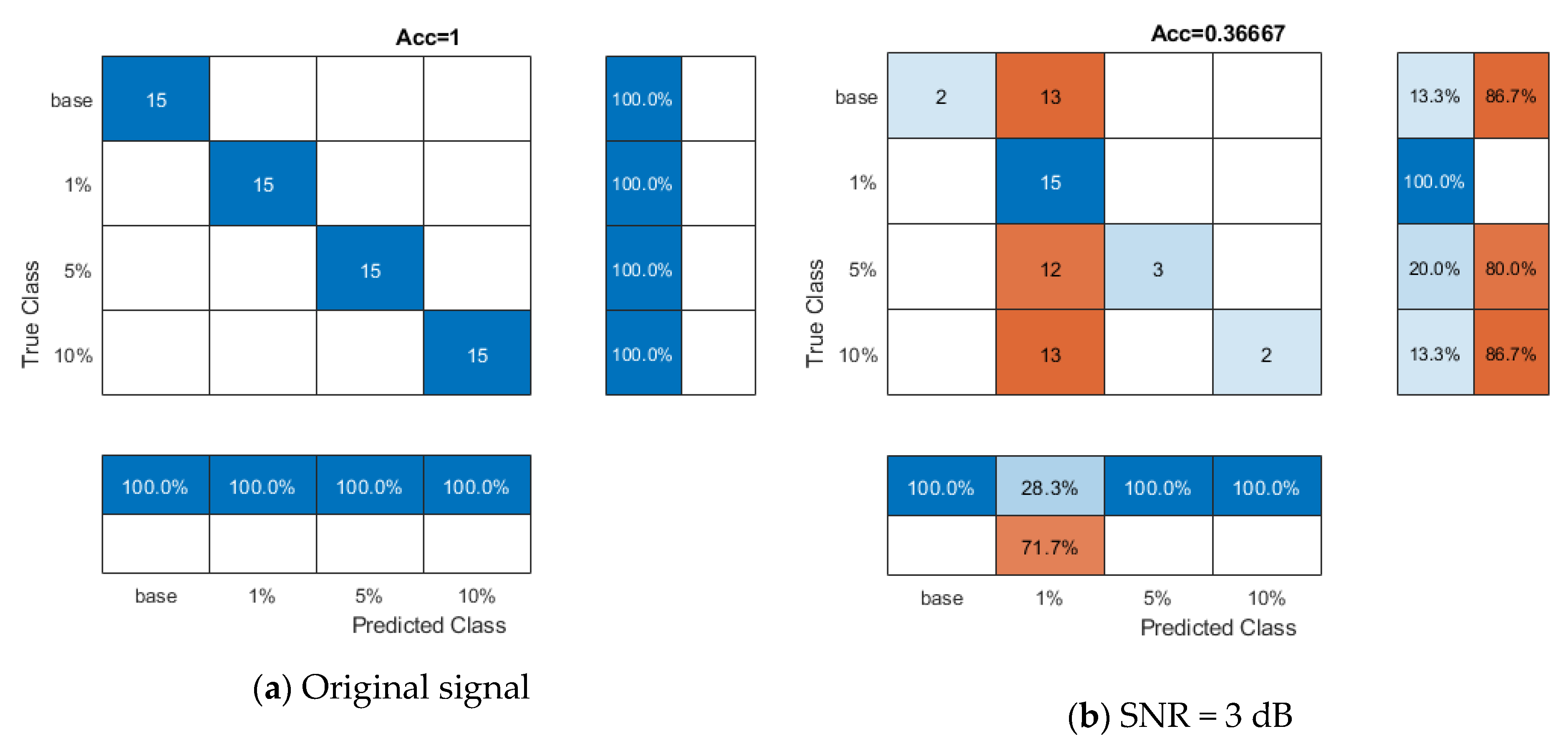
The confusion matrix serves as a robust tool for assessing the classification performance, enabling the quantification of overlaps in categorization [
53]. This numerical framework is pivotal in analyzing error distributions within classification tasks [
54]. It is utilized extensively in various machine learning contexts, including neural networks, decision trees, Bayesian methods, and support vector machines [
55]. Ahmad et al. applied modularized induction techniques using the confusion matrix for pretrained CNNs [
56]. This matrix can be used to determine the classification accuracy as follows:
where
signifies the ratio of correct negative predictions,
stands for the ratio of incorrect positive predictions,
denotes the ratio of precise negative predictions, and
indicates the ratio of precise positive predictions.
The Area Under the Receiver Operating Characteristic Curve (AUC), a crucial assessment tool in classification tasks, is also introduced. The AUC quantifies the model’s proficiency in distinguishing between classes by measuring its capacity to assign higher probabilities to positive instances. A higher AUC score, closer to 1, signifies superior discrimination and overall model performance. This inclusion broadens the scope of our evaluation, offering deeper insights into the model’s classification ability and its adaptability to class imbalances, ensuring a more comprehensive analysis of its effectiveness and reliability.
5. Further Discussion of Pipelines under Different Embedment
To further evaluate the robustness of the effectiveness of the CNN-LSTM model, CNN and LSTM models were trained, and more complex models were constructed in COMSOL to produce more training data. The established parameter of the COMSOL model was kept the same as in Case 1, as shown in
Figure 3. The only difference was the pipeline embedding materials. The soil embedding materials [
34] were changed to soft clay, stiff clay, loose sand, dense sand, and concrete [
58,
59,
60].
Table 8 shows the properties of the embedding materials.
5.1. Signal Characteristics of the Pipes under Different Embedment Materials
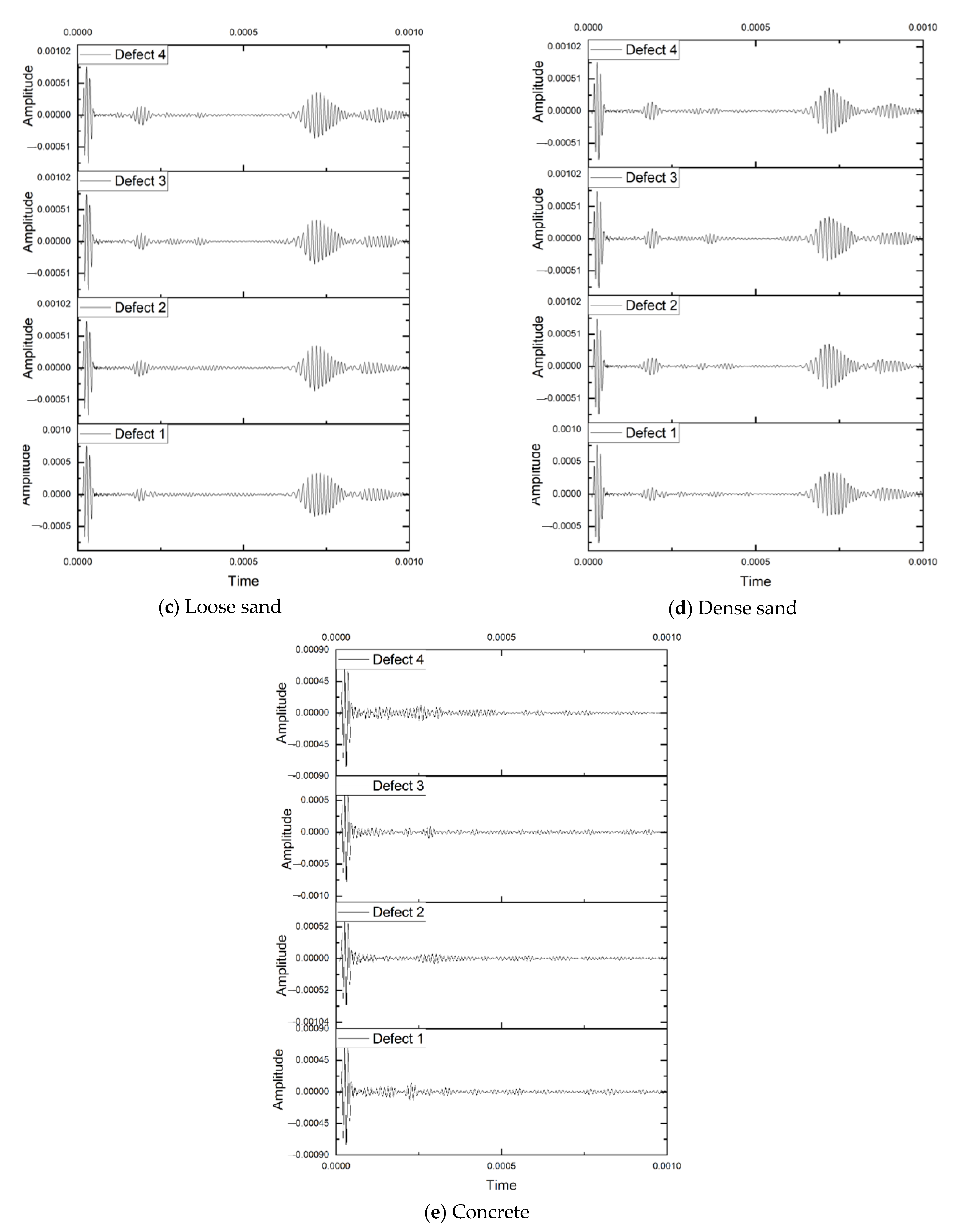
Figure 12 shows the pipeline waveforms with defect 4 with 10% severity under soft clay, stiff clay, loose sand, dense sand, and concrete embedment. It can be seen the signals of soft clay, stiff clay, loose sand, and dense sand have the most obvious defect reflection area and boundary reflection area, while the signals of concrete embedment have no such trend. It was mostly due to the concrete’s substantially higher attenuation of sand and concrete, which results from the directed waves’ higher energy leakage to the embedment and energy loss absorbed by concrete and sand in comparison to soil. Leinov’s research also confirmed this [
61].
5.2. Impacts of Embedment Conditions on Classification Performance of Deep Learning Models
As shown in
Figure 13, the performance for the cases with embedding soil, soft clay, stiff clay, loose sand, and dense sand is almost the same. It can be also demonstrated in
Figure 12, the waveforms of embedding soil, soft clay, stiff clay, loose sand, and dense sand are almost the same. And, the CNN-LSTM model has the best training performance and the highest accuracy in comparison with the CNN and LSTM models under high noise interference for the cases of embedding soil, soft clay, stiff clay, loose sand, and dense sand. For instance, when the noise level rises to 6 dB for the cases with embedding sand, the performance of the CNN-LSTM model improves by 12.2% compared to the CNN model and 17.9% compared to the LSTM model. At the same noise level for the cases with embedding concrete, the CNN-LSTM model outperforms the CNN and LSTM models by 12.1% and 6.1% higher, respectively. The results show the CNN-LSTM hybrid has the best classification performance.
Furthermore, the accuracies of the three models for the cases with embedding soil, soft clay, stiff clay, loose sand, and dense sand are much higher than the accuracies of the three models for the cases with embedding concrete. When SNR is equal to 12 dB, the performance of the three models for the cases with embedding soil improves by 8–11% compared to that for the cases with embedding concrete, which is consistent with Zhang’s early findings [
4].
5.3. Further Discussion about the Applicability to Different Metallic Materials
Our proposed ultrasonic-guided wave testing method has shown promise for the detection of welding defects in pipelines. While the study primarily focuses on a specific material, Ti-6Al-4V, which is commonly used in pipelines, it is essential to consider the broader applicability of this method to a range of metallic materials, including steel, aluminum, and copper, which are frequently employed in various industrial settings.
Advantages of the Proposed Method for Different Metallic Materials: firstly, the method’s non-destructive nature makes it adaptable to a variety of metallic materials without causing damage [
62]. Secondly, ultrasonic-guided waves have demonstrated sensitivity to material variations, enabling the detection of defects in different metals. Thirdly, the method’s ability to operate at various frequencies allows for versatility when dealing with different materials, each having its own acoustic characteristics.
However, there are still limitations and challenges with non-ferrous metals. Non-ferrous metals, such as aluminum and copper, have distinct acoustic properties that may require specific calibration and signal processing techniques. Furthermore, materials with high electrical conductivity, like copper, can affect the propagation of ultrasonic waves. Mitigating this influence is an ongoing challenge. Last but not least, non-ferrous metals may exhibit higher signal attenuation compared to ferrous materials, impacting the range and quality of defect detection.
As a result, to broaden the scope of our method’s applicability, further research is needed to investigate and address the specific challenges associated with non-ferrous metals. This includes the development of material-specific calibration techniques and signal processing algorithms to enhance the accuracy and reliability of defect detection.


