Article

Modeling of Heat Flux in a Heating Furnace

1
Department of Thermal Technology and Gas Industry, Institute of Metallurgy, Faculty of Materials, Metallurgy and Recycling, Technical University of Kosice, Letná 9, 042 00 Kosice, Slovakia
2
Department of Process Technique, Faculty of Manufacturing Technologies with a Seat in Presov, Technical University of Kosice, Bayerova 1, 080 01 Presov, Slovakia
*
Author to whom correspondence should be addressed.
Computation 2023, 11(7), 144; https://doi.org/10.3390/computation11070144
Submission received: 2 July 2023 / Revised: 14 July 2023 / Accepted: 14 July 2023 / Published: 17 July 2023

Abstract

:
Modern heating furnaces use combined modes of heating the charge. At high heating temperatures, more radiation heating is used; at lower temperatures, more convection heating is used. In large heating furnaces, such as pusher furnaces, it is necessary to monitor the heating of the material zonally. Zonal heating allows the appropriate thermal regime to be set in each zone, according to the desired parameters for heating the charge. The problem for each heating furnace is to set the optimum thermal regime so that at the end of the heating, after the material has been cross-sectioned, there is a uniform temperature field with a minimum temperature differential. In order to evaluate the heating of the charge, a mathematical model was developed to calculate the heat fluxes of the moving charge (slabs) along the length of the pusher furnace. The obtained results are based on experimental measurements on a test slab on which thermocouples were installed, and data acquisition was provided by a TERMOPHIL-stor data logger placed directly on the slab. Most of the developed models focus only on energy balance assessment or external heat exchange. The results from the model created showed reserves for changing the thermal regimes in the different zones. The developed model was used to compare the heating evaluation of the slabs after the rebuilding of the pusher furnace. Changing the furnace parameters and altering the heat fluxes or heating regimes in each zone contributed to more uniform heating and a reduction in specific heat consumption. The developed mathematical heat flux model is applicable as part of the powerful tools for monitoring and controlling the thermal condition of the charge inside the furnace as well as evaluating the operating condition of such furnaces.

1. Introduction

Heating furnaces can be divided into various groups based on selected criteria. One of the criteria is the heating mode, which is determined by the technological requirements. Convective or radiant heating can predominate in the furnace. The importance of the correct heating mode is related to the uniformity of the temperature field within the charge and the heating time. These two factors are crucial for intensifying the heating process and determining the operational economy of such a furnace [1,2,3].
Among the important types of heating furnaces are pusher furnaces. Pusher furnaces have undergone development, with their geometry and parameters based on technological needs. Various construction types of pusher furnaces have been described by authors in [2] and [3]. An important common factor is the energy consumption for heating the charge. Therefore, possibilities for reducing energy consumption are explored, such as by installing more efficient insulation and refractory materials [4,5,6]. Another option is to achieve better heat distribution through the installation of new burners [7].
Pusher furnaces are continuous heating furnaces used for heating slabs to the rolling temperature. They feature a floor-level balancing zone, a radiant ceiling, bottom heating, front loading, and front unloading using inclined skids or an unloading machine [3].
Pusher furnaces are used for heating square or rectangular billets for rolling and forging. Furnaces for heating thin material (50–100 mm) with large lengths (up to 12,000 mm) typically have a slight slope, usually around 6–7°, towards the extraction opening to prevent the material from sticking and reduce the required pressing force. The processed materials have the following dimensions: thickness of 40–400 mm, width of 40–2500 mm, length of up to 15,000 mm, and weight of 0.05–40 tons [3,6].
The heating of slabs in pusher furnaces depends on subsequent forming processes and the desired final heating temperature before hot rolling. It is influenced by various factors, especially the type of steel. The temperature should be maintained at approximately 100–150 °C below the solidus curve. The upper limit is constrained by grain growth, the risk of overheating due to thermal stresses, and increased oxidation. The lower limit of heating is determined by the permissible temperature at the end of processing, depending on the steel grade. Pusher furnaces play a crucial role in the rolling process. The furnace must deliver the required quantity of slabs with the desired heating quality within a specified time frame, forming an integral part of the production line [3,6].
The heating of metal in a pusher furnace is a flow process characterized by the movement of heated material through a series of heating zones arranged spatially. Control variables (e.g., zone temperature) are also distributed in space, acting on all slabs simultaneously along the entire length of the heating zone, which are at different thermal states [3,6].
The heating of slabs in a pusher furnace depends on the forming process. This process must be carried out to achieve the following objectives [6]:
-
Uniform desired properties along the length of the strip are considered for the rolling direction and transverse direction (yield strength, elongation, toughness);
-
The uniform geometric shape of the strip (thickness, width) along its entire length;
-
Maximum line performance with minimal energy consumption and minimal material losses [8,9].
The working space of the pusher furnace is divided into several temperature zones. The material passes through four consecutive zones: preheating, heating (upper and lower heating), balancing, and holding zone, where irregularities occurring during material heating are leveled out [3,4,6].
The preheating zone, into which the cold charge enters, serves two main purposes and is characterized by a gradual increase in the flue gas temperature. The first purpose is the slow heating of the pre-rolls up to a temperature of 500 °C, where there is a risk of thermal stress damage to the steel. The charge is heated gradually to avoid an undesirable temperature gradient between the surface and the center of the pre-roll. The second function is the utilization of flue gas heat.
From the preheating zone, the charge proceeds to the heating zone, where the surface of the pre-rolls is rapidly heated to the desired heating temperature. Upon exiting the heating zone, the pre-rolls are unevenly heated, with a significant difference between the surface and center temperatures. The balancing zone is responsible for reducing this temperature difference. It is an important part of the pusher furnace and serves to eliminate shadows during the heating of the pre-rolls on the skids. For rolling purposes, it is required that the temperature gradient along the height of the pre-rolls does not exceed 1 to 3 K·cm−1. The power input into the balancing zone is chosen so that the flue gas temperature is 50 to 70 K higher than the heating temperature. The surface temperature remains unchanged, while the center temperature slowly approaches it [1,3,6].
The characteristics of pusher furnaces indicate numerous factors that need to be incorporated into the control of such thermal units.
The authors in [8,9] address the factor of scale in the charge heating process. Appropriate heating parameters allow the formation of deposits to be controlled during the heating process and ensure the predictability of the effects on the material.
For a more complex analysis of the heating process, it is necessary to make an energy and material balance of the charge heating [1]. This is based on data from measurements on heat aggregates, which serve to verify calculations. In many studies, the authors devoted themselves to the creation of balance [10,11,12] and prediction models [13,14], the basis of which was internal and external heat exchange. Some authors focused on the analysis of furnace work [10,15] and the creation control systems [12,13,16,17,18] for heating in pusher furnaces. Optimization models [19,20] or, currently, CFD modeling [14,15] are used for the analysis of the work of the thermal aggregate. Another suitable method is work analysis based on heat losses [10], from which the efficiency of the slab heating process is determined. Due to the non-linearity of the parameters of the heated material, it is necessary to apply suitable non-linear equations in the calculations [16,17], which are also part of control and prediction models [12,13,14,18].
It follows from the works [10,11,12,13,14,15,16,17,18,19,20] that some heat aggregates have a different heating mode, and therefore the mathematical models created are specific.
A big problem with the created models is downtime when removing the heated slabs from the furnace. This is due to a malfunction (technical defect) on the device or in another device during slab processing. In such cases, it is possible to adjust the heating mode using some prediction, control, and control models.
The authors aim to create a mathematical model for evaluating heat fluxes on the massive charge based on temperature profile measurements. The calculation algorithm is based on internal heat exchange. The developed model is intended to serve as a supporting tool for monitoring the duration of the heating process, and the results of the calculations will be used as a basis for intensifying the heating of the charge in the pusher furnace. The created model should be applicable to similar types of charge heating furnaces with moving charges.

2. Materials and Methods

Optimal parameters for heating the slabs in a pusher furnace, including the heating time of the material and specific energy consumption, are dependent on the following factors [1,3]:
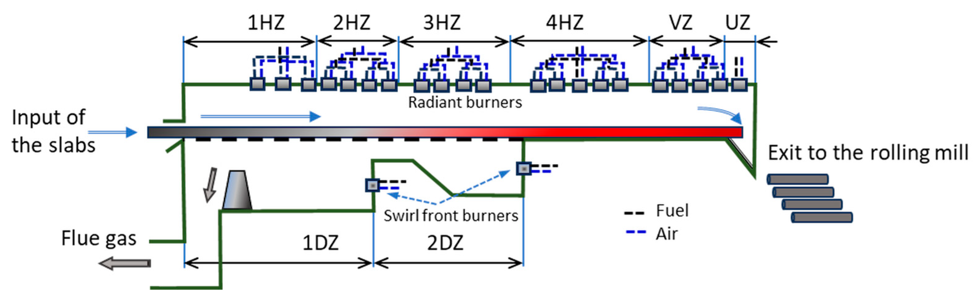
  • Temperature field in the furnace working space (heat inputs in individual furnace zones);
  • Composition of the furnace atmosphere (excess combustion air, fuel composition, and fuel combustion);
  • Inlet temperature of the slabs;
  • Slab temperatures above the skids (condition of the furnace cooling system);
  • Type of steel.
These factors significantly influence both the external and internal heat exchange during the slab heating process in pusher furnaces. Conducting a thorough analysis of these factors allows for the identification of key factors that can intensify the slab’s heating process.
The internal heat exchange of the slabs is characterized by the temperature field within the slab, while the external heat exchange is determined by the temperature profile in the furnace working space and the heat flux incident on the slab’s surface. By evaluating the heat exchange along the length of the furnace during the heating process, temperature measurements taken within the slab between the skids serve as crucial reference data.
In order to enhance slab heating in pusher furnaces, measurements of thermotechnical variables were conducted. The following parameters were measured [1,3]:
-
Type and characteristics of the charge material;
-
Fuel type, fuel composition, and heat inputs in different furnace zones;
-
Quantity of air in each furnace zone and air temperature;
-
Furnace temperature in each zone;
-
Inlet surface temperature of the charge material;
-
The oxygen content of the flue gas at the furnace flue gas outlet;
-
Rolling temperature behind the 5th rolling table;
-
Quantity of cooling water, as well as inlet and outlet water temperatures;
-
Temperatures within the slab.
These measurements provide essential data for understanding and optimizing the slab heating process in pusher furnaces.
To measure the temperature profile inside the material, a test slab made of low-carbon steel 11-375 was utilized. This steel contains a carbon content of up to 0.09% by weight and is accurately defined according to the STN 41-1375 standard [21]. The measurements were carried out with the aim of intensifying the heating of slabs in pusher furnaces. The measurements took place inside the furnace during its operation with the test slab, and the temperatures inside the slab were continuously measured from the entry point into the furnace until its expulsion at the furnace outlet. The measuring device used for these temperature measurements was the data logger TERMOPHIL-stor type 4468/4469 (Ultrakust Electronic GmbH, Gotteszell, Germany), capable of recording data from 6 measuring points. The measuring points within the slab are schematically illustrated in Figure 1. Thermocouples 1–3 were positioned outside the skids at a distance of 650 mm from the right edge of the slab, while thermocouples 4–6 were positioned at a distance of 1300 mm from the right edge of the slab (above the skids). Measurement points 1, 4, 3, and 6 were positioned at a distance of 25 mm from the upper and bottom surfaces of the slab. Measurement points 2 and 5 were positioned in the center of the slab. The selection of measurement locations was specified in order to capture the temperature distribution within the slab, unaffected by the cooling system of the skids, as well as the temperature distribution directly above the skids. This approach enabled the acquisition of more comprehensive insights into the slab heating process.
Due to the high temperatures in the furnace, type S thermocouples (PtRh10-Pt) were employed for temperature measurement at the measuring points in the test slab. Type S thermocouples can be used up to a temperature of 1600 °C.
The parameters of the test slab were as follows:
-
Dimensions: 8000 × 1540 × 200 mm
-
Weight: 15.5 t
The values of the temperatures at all measuring points were registered at one minute intervals.
After the test slab was pushed out of the furnace, the data logger was removed from the slab, and the measurement was completed. By synchronizing the time, a section was marked in the acquired data that corresponded to the actual time the slab stayed in the pusher furnace.
Figure 2 shows the location of the slabs and their movement, which was carried out by a push button at the furnace entrance. At the outlet, the slab slides down the inclined surface onto the roller transport conveyor. The above method of exiting the slabs from the pusher furnace before the reconstruction caused large mechanical shocks when they hit the roller conveyor.
The heating of the charge in the pusher furnace is provided by combined heating by overhead radiant and underfloor swirl front burners [7]. For each zone, a separate heating mode is set. In the high-temperature field, the furnace atmosphere is also adjusted to prevent excessive scale formation [4,9]. During heating, scale affects the transfer of the body to the inside of the slab and thus can cause differences in the temperature field across the cross-section of the heated material [6,9].
Figure 3 illustrates the differences between the measured temperatures outside the skids (measuring points 1–3) and directly on the water-cooled skids (measuring points 4–5). The water in the skids creates temperature shadows that need to be eliminated in the balancing zone (VZ).
During the measurement, the residence time of the slab in the furnace was 171 min, with a residence time in the double-sided heating zones of 100 min. The temperatures between the skids reached 1258–1280 °C at the end of the heating process, while above the skids, temperatures ranged from 1244 to 1272 °C. The maximum temperature difference across the thickness of the slab was 42 °C.
The analysis of the slab heating process in the pusher furnaces was conducted through comprehensive measurements of furnace operation and temperature profiles in the slabs at various heating times. These measurements subsequently led to the design and implementation of reconstruction, involving adjustments to specific parameters of the pusher furnace. A schematic representation is shown in Figure 4.
The main objective of the reconstruction is primarily to reduce the specific energy consumption during heating, improve the quality of slab heating, and reduce losses due to scaling [9]. After the reconstruction of the pusher furnace, the active length of the furnace changed from 32.5 m to 34 m. From the schematic representation in Figure 4, one can also observe the change in the furnace profile in the vault and the lower zone. The added partitions have intensified heat exchange, especially through convection. The flue gases are now forced to flow more around the slabs. The method of slab removal from the furnace has been modified. The insulation of the water-cooled skids and the burner system has been improved.
The furnace reconstruction at its discharge end consists of the elimination of the inclined slips and the prolongation of the furnace nest part. The insulation of the lower face after combustion fuel burners provides higher-quality slab heating, and the temperature difference between the upper and lower slab sides will decrease [3,9].
In order to verify the appropriateness of the changes in the parameters of the pusher furnace, control measurements were carried out using a test slab. The location of the thermocouples in the test slab is shown in Figure 5.
Figure 5 shows the schematic layout of measurement points in the test slab. The material of the used test slab had the same properties as in the case of the pusher furnace before reconstruction, which was low-carbon steel 11-375 [21]. In this case, a test slab with a thickness of 220 mm was employed. The temperature field was recorded at unaffected measurement points 1–3, while the temperature field influenced by the cooling system of the skids was observed at measurement points 4–6.
Figure 6 shows the temperature curves in the test slab at individual measurement points along the length of the furnace. The temperatures indicated in Figure 6 as t1t6 correspond to the respective measuring points 1–6 as illustrated in Figure 5. The heating is set up in such a way that the temperature in the slab increases only in the region of uniform heating, indicated by 20 m. During this heating phase, the surface temperature of the slab reaches approximately 1200 °C. Subsequently, in the following zones during the heating process, the temperature inside the slab equalizes and reaches the desired temperature for rolling.

Determination of Heat Fluxes on the Charge Surface

Knowledge of the course of heat fluxes falling on the charge surface allows charge heating intensification, e.g., Varga [1]. In this work, the authors focused on the solution of internal heat exchange, which was based on the fundamentals of the 1st Fourier law of heat transfer [22,23,24]. Due to the unsteady heat flux, the 1st Fourier law cannot be applied. Therefore, an alternative solution was sought, which was based on the measured temperatures and the determination of the material’s enthalpy. When estimating heat fluxes falling on the charge surface, the way out is the course of the measured temperature in the slab between skids. Since the temperature distribution along the slab height follows a quadratic pattern, the entire temperature profile across the slab cross-section can be determined from just 3 measured values, as described by the following equation:
t = k   x 2 + q   x + p .
The coefficients k, q, and p are obtained by solving Equation (1) for values of 3 temperatures from 3 measuring points (a set of 3 equations of 3 variables).
As the temperature course along the slab cross-section is described by a quadratic equation, the temperature at a certain distance from the slab surface, x m i n , is minimal at t m i n .
The t m i n value is determined from:
t m i n = d t d x = 0 .
The distance x m i n is calculated from Equation (1) when the substitution t = tmin is made.
For the calculation of heat fluxes, it is assumed that up to the distance x m i n , the heat flux from the upper side q h is effective, and up to the distance ( s x m i n ), the heat flux from the lower side q d is effective. This is clearly illustrated in Figure 7.
The heat fluxes are calculated according to the following equations:
q h , i = c p   h , i + 1   t ¯ h , i + 1 c p   h , i   t ¯ h , i ρ ¯ h   x m i n   τ ,
q d , i = c p   d , i + 1   t ¯ d , i + 1 c p   d , i   t ¯ d , i ρ ¯ d   s x m i n   τ ,
where:
i—time index;
τ —length of the time interval (s);
q h , i and q d , i —the heat flux from the upper side to the lower side (W m−2);
c p   h , i —the mean specific heat capacity at the t ¯ h , i temperature (J·kg−1 K−1);
c p   d , i —the mean specific heat capacity at the t ¯ d , i temperature (J·kg−1 K−1);
t ¯ h , i + 1 —the mean charge temperature on the thickness x m i n at time τ i + 1 (°C);
t ¯ h , i —the mean charge temperature on the thickness x m i n at time τ i (°C);
t ¯ d , i + 1 — the mean charge temperature on the thickness ( s x m i n ) at time τ i + 1 (°C);
t ¯ d , i — the mean charge temperature on the thickness ( s x m i n ) at time τ i (°C);
ρ ¯ h —charge density at the mean temperature t ¯ h , i + 1 + t ¯ h , i 2 in the time interval ( τ i , τ i + 1 ) (kg m−3);
ρ ¯ d —charge density at the mean temperature t ¯ d , i + 1 + t ¯ d , i 2 in the time interval ( τ i , τ i + 1 ) (kg m−3);
s—slab thickness (m).
The mean charge temperatures from the upper side t ¯ h , i on the thickness x m i n and from the lower side t ¯ d , i on the thickness ( s x m i n ) are obtained by solving Equation (1) as follows:
t ¯ h , i = k x m i n , i 3 3 + q x m i n , i 2 2 + p   x m i n , i t o , i t m i n , i .
To shorten the following equation, substitutions are used:
a 1 = s x m i n 3 ; a 2 = s x m i n 2 ; a 3 = s x m i n ,
t ¯ d , i = k a 1 3 + q a 2 2 + p   a 3 t s , i t m i n , i ,
where t o , i represents the temperature of the upper surface of the slab in Equation (5), and t s , i represents the temperature of the lower surface of the slab in Equation (6) (°C).
During the experimental measurements, a slab made of low-carbon steel was used, which exhibits nonlinear thermophysical properties, especially in terms of thermal capacity (cp). Therefore, it was necessary to establish temperature dependencies for this material. Some of the literature divides the temperature range into smaller intervals and utilizes linearized dependencies in their models. In this case, tabulated values from [25] were employed, and temperature dependencies for the mean specific heat capacity of low-carbon steel with a carbon content of 0.08 mass% were obtained through regression analysis. The temperature dependence of the heat capacity was addressed by employing a 3rd degree polynomial, as outlined in Equation (7), which effectively captured the behaviour of the provided data in [25]. The coefficients necessary for Equation (7) were determined and are presented in Table 1. To enhance the precision of the specific heat capacity calculations, it seemed most appropriate to divide the temperature interval as shown in Table 1.
c ¯ p = a + b   t ¯ + c   t ¯ 2 + d   t ¯ 3
To calculate the density ρ (kg m−3) of low-carbon steel, the following relationship can be used:
ρ = 7886,285 0,35   t ¯ .
When deriving Equations (3) and (4) for the heat flux estimation, the law of energy conservation is applied, which means that the charge enthalpy can be changed only due to the heat supplied to the charge surface. From the calculated heat fluxes q h and q d the total heat amount falling on the surface unit is determined according to the expression:
q = q h q d .
From the measured and calculated results obtained, graphical relationships were created.
The correctness of the proposed method for the solution of the heat fluxes is also confirmed by the following calculation:
The change of the specific enthalpy i can be estimated according to the expression:
i = c p , k t ¯ k c p ,   p t ¯ p ,
c p ,   p —the mean specific heat capacity at the beginning of heating (J kg−1 K−1);
c p , k —the mean specific heat capacity at the end of heating (J kg−1 K−1);
t ¯ k —the mean slab temperatures at the end of heating (°C).
t ¯ p —the mean slab temperatures at the beginning of heating (°C).
The change of enthalpy i can be estimated according to the relationship:
i = 1 = 1 n i h , i + i d , i ,
where:
i h , i —change of the charge-specific enthalpy at the heat flux from the upper side for the time interval (J kg−1);
i d , i —change of the charge-specific enthalpy at the heat flux from the lower side for the time interval (J kg−1).
For i h , i and i d , i the following calculation is applied:
i h , i = c p   h , i + 1   t ¯ h , i + 1 c p   h , i   t ¯ h , i x m i n , i s ,
i d , i = c p   d , i + 1   t ¯ d , i + 1 c p   d , i   t ¯ d , i s x m i n , i s .
If we compare the equations for calculating heat fluxes (3) and (4) and the change in enthalpy (12) and (13), the following holds true:
i = q ρ i   s   τ .
When comparing the i values calculated using Equations (10) and (11), it is observed that there is an approximate difference of 0.5% attributed to calculation inaccuracies. This indicates that the proposed methodology for calculating the heat fluxes falling onto the charge surface from the obtained measurements can be considered accurate. This finding is consistent with the work of Varga [1].

3. Results and Discussion

Based on the mathematical model created and the measured temperatures inside the slab, the results of the heat flux profiles were obtained as a function of the slab heating time in the heating furnace. When performing calculations using the mathematical model, only temperatures outside the skids were considered, as the temperatures inside the slab or the heat dissipation through the water-cooled slides would influence the results, which are not accounted for in this model.
From the processed measurement results, the following graphical dependences have been constructed:
-
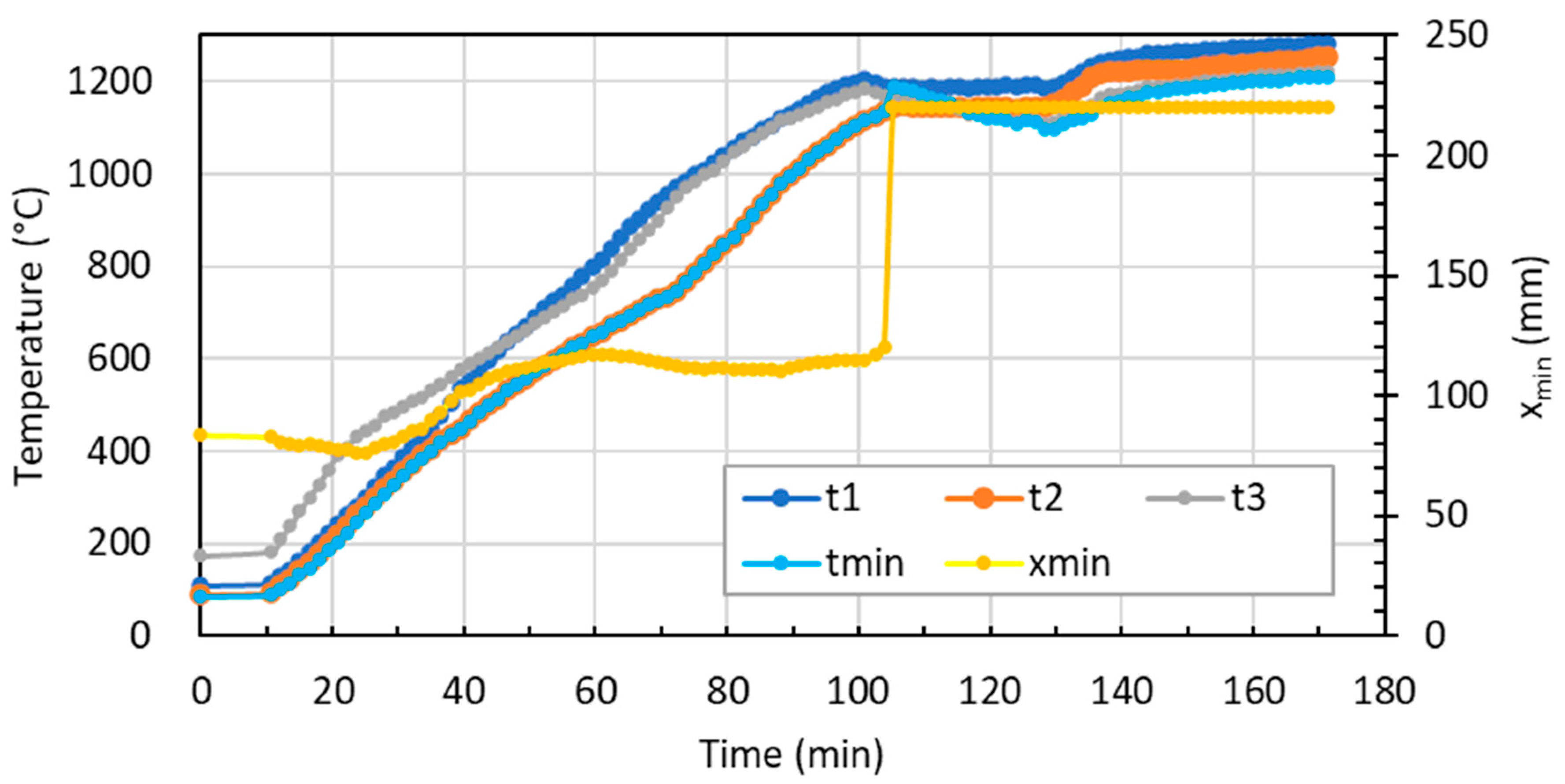
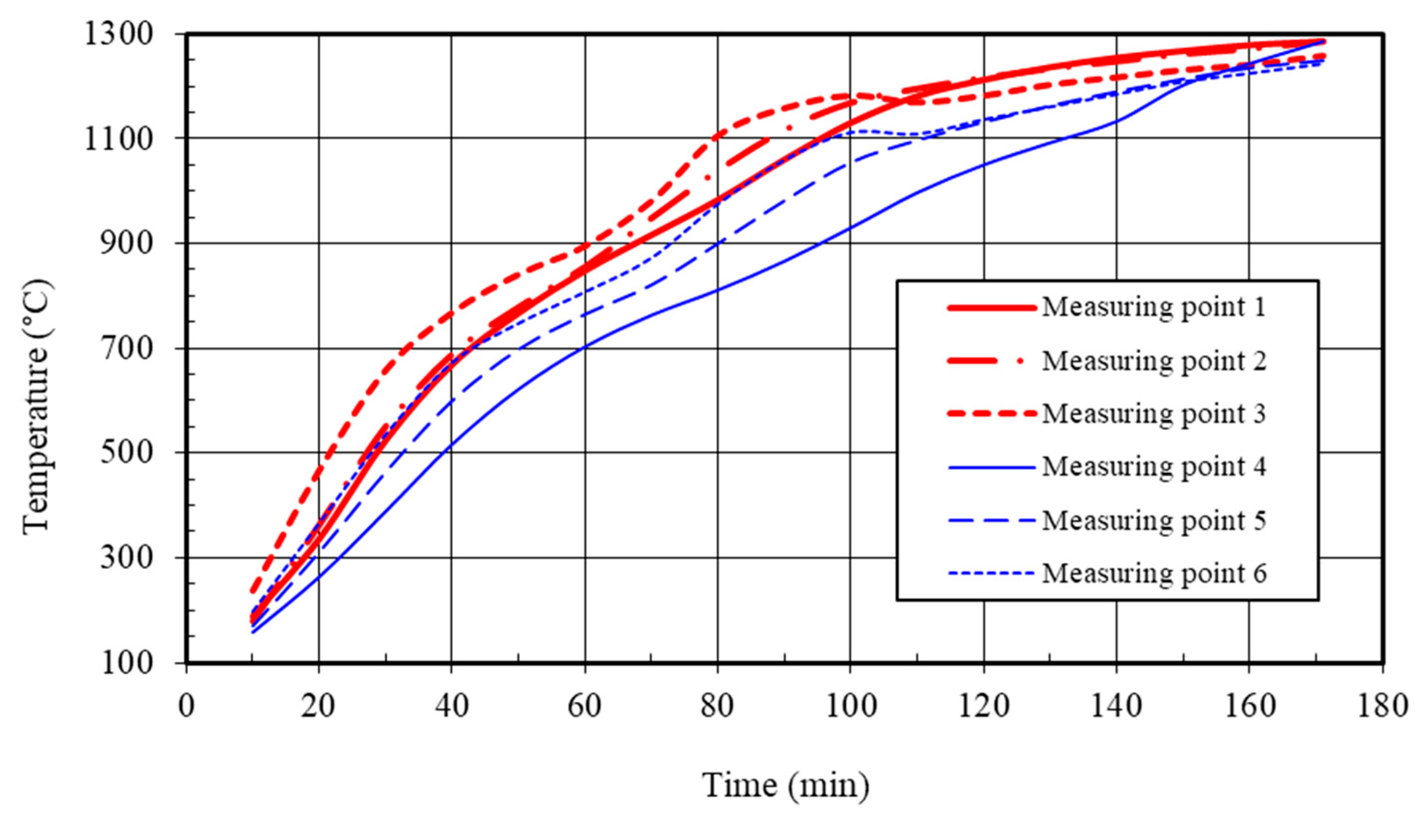
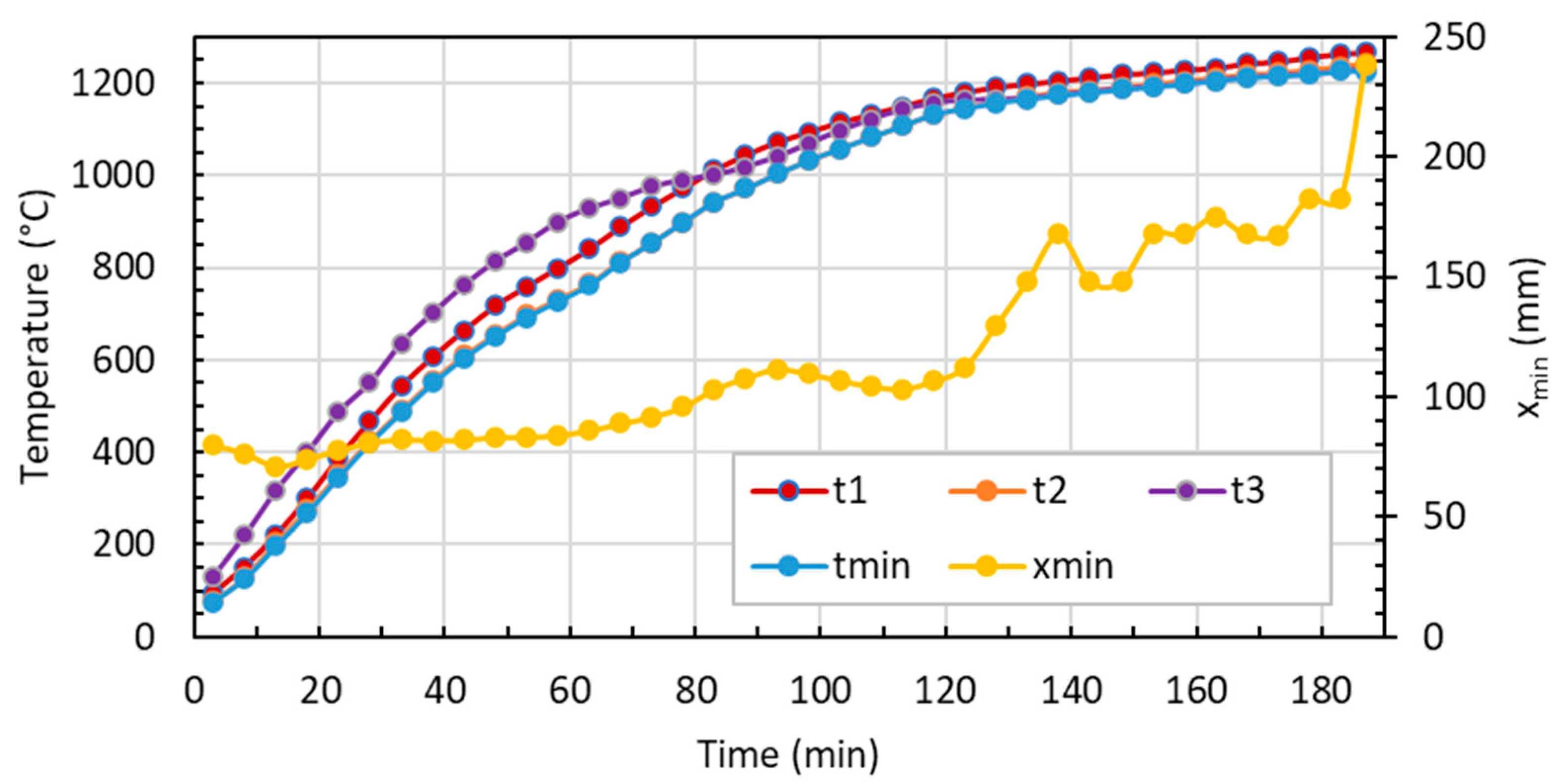
The temperature courses in the slab in dependence on the duration of before reconstruction and after reconstruction of the pusher furnace;
-
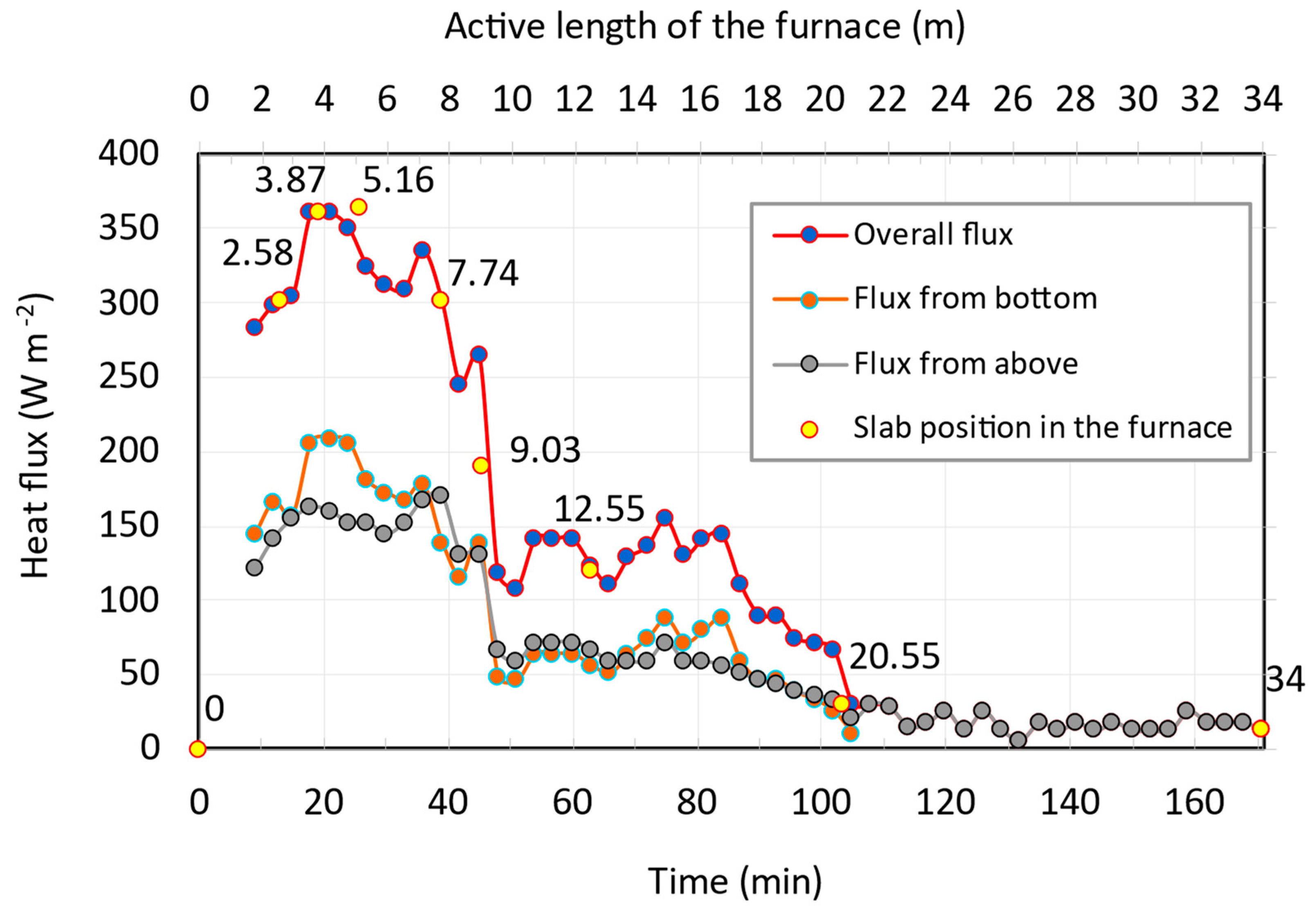
The heat flux courses to the slab surface in dependence on the duration of heating before reconstruction and after reconstruction of the pusher furnace.
Figure 8 and Figure 9 show the results for the test slab measurement with a heating time of 187 min. This is because of the heating comparison shown in Figure 3, where the residence time of the slab in the furnace was 171 min.
In Figure 8, it is possible to observe the temperature rise in the slab during the measurement as well as the calculated minimum temperature tmin and the calculated slab thickness xmin needed to calculate the heat fluxes. Temperatures t1–t3 correspond to the temperatures at measuring points 1–3 in the slab, which are in Figure 1.
By comparing different residence times in the pusher furnace, it was found that the temperature profiles measured over the furnace length are very similar. From the thermomechanical analysis of the heating of the slabs during the measurements with the test slab (Figure 8 and Figure 9), it follows that there is an increase in heat fluxes from the top and bottom up to a heating time corresponding to a distance of approximately 4 m. In this area of the furnace, there are no burners, and the heat mainly comes from radiation from other parts of the furnace. The increase in heat flux corresponds to an increase in furnace temperatures in that furnace region. In the lower part of the furnace, this distance corresponds to the width of the exhaust flue gas channel.
From Figure 9, it is evident that until a heating time corresponding to the width of 1DZ, the heat fluxes from the bottom are considerably higher than the heat fluxes from the top, which is also reflected in the higher surface temperatures at the bottom, approximately 100 °C higher than the surface temperatures at the top (Figure 9). Furthermore, Figure 9 shows that the heat fluxes in 2DZ are lower than the heat fluxes in the upper zones of that region, resulting in a slight increase in the surface temperatures of the slabs at the bottom compared to the surface temperatures of the slabs at the top (Figure 8). Additionally, Figure 9 indicates that the heat fluxes in 2DZ are lower than the heat fluxes in the upper zones of that region, causing only a slight increase in the surface temperatures of the slabs at the bottom compared to the surface temperatures of the slabs at the top (Figure 8). The surface temperatures of the slabs at the top are higher than those at the bottom at the end of 2DZ, which negatively affects the residence time in 4HZ and VZ, considering only the upper heating method in these zones.
In the 4HZ and VZ regions, the heat fluxes are approximately equal, resulting in only a slight increase in surface temperature at the top. The furnace temperature is relatively uniform throughout this region. Similar results were obtained for low-carbon steels in other measurements.
From this analysis, it can be concluded that such a regime is not suitable in terms of energy consumption. This controlled heating leads to an increased temperature of the exhaust gases leaving the furnace, indicating increased heat losses through the exhaust gases. To reduce specific energy consumption for heating, it is necessary to regulate the heat inputs in individual zones in such a way that:
-
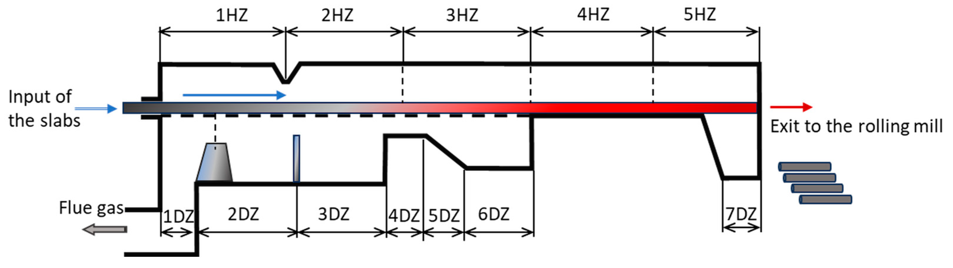
The heat fluxes from the bottom and top are approximately equal up to a distance of 1DZ;
-
The heat fluxes from the bottom are slightly higher than the heat fluxes from the top in the 2DZ, ensuring higher surface temperatures for the slabs at the bottom and the top at the end of the 2DZ.
To achieve this, it is necessary to reduce the heat input in 1DZ and increase the heat input in 2DZ, resulting in a smoother increase in temperatures in the slab.
Based on measurements of heat inputs in individual zones of the furnace, it can be observed that the heat input in 1DZ was 25.7%, in 1HZ it was 31.4%, and in 2HZ it was 16.6%. Considering that there is a high heat consumption for cooling the skids and other parts of the cooling system in 1DZ, the heat fluxes and surface temperatures of the slabs from the top should be higher than those from the bottom. This fact indicates that significant transfers of heat inputs (or fresh combustion gases) occur through the free spaces between the furnace walls and the charge, from the upper zones to the lower zones. These transfers of heat inputs require studying the flow of combustion gases in the working space of the furnace, depending on the overall furnace regime. Understanding the flow pattern is only possible through a physical furnace model that allows simulation for different furnace heat regime variants or through advanced CFD simulation software [14,15].
Considering that the cooling system of the pusher furnace was not insulated before the reconstruction, there was increased heat consumption, especially in 1DZ and 2DZ. Insulating the cooling system can reduce the heat input in 1DZ and provide the possibility of increasing the heat input in 2DZ, thus ensuring uniform heating of the slabs up to a distance of approximately 1DZ and slightly increased bottom heating of the slabs in the 2DZ region. Insulating the cooling system and making subsequent adjustments to the furnace heat regime will reduce the overall thermal energy consumption and, therefore, decrease the specific energy consumption for heating the slabs in pusher furnaces. It will also provide a more uniform temperature distribution across the slab section at the end of the heating process and shorten the heating time.
Figure 10 shows the t1t3 temperature time histories corresponding to the temperatures from measurement points 1–3 in the slab according to Figure 5. For the calculation of tmin and xmin, the same calculation methodology was applied as in Figure 8.
The comparison of the slab heating curves before reconstruction in Figure 8 and after reconstruction in Figure 10 reveals that the thermal regime of the furnaces after reconstruction is more favorable due to a more uniform temperature rise in the slab area during double-sided heating.
From the comparison of the heat flux curves in Figure 9 and Figure 11, a significant change in the decrease of heat flux in the double-sided heating region can be observed.
Comparing the maximum total heat fluxes, a 63% decrease can be observed, and similarly for the upper (59% decrease) and lower heat fluxes (65% decrease). The mathematical model is applicable for the evaluation of the heating from the internal heat exchange point of view. However, the heat flux drops do not take into account another parameter affecting the specific energy savings. Therefore, it is only an auxiliary but effective tool for more complex mathematical models.

4. Conclusions

The mathematical model created for evaluating the thermal regime of pusher furnaces for slab heating prior to rolling provides valuable insights into optimizing the heating process. By combining modern measurement techniques with the mathematical model, important data was gathered to assess the operational state of these furnaces, with a focus on specific energy consumption for slab heating.
The conducted measurements, subsequent calculations, and evaluation of the results have shed light on the fundamental principles of slab heating. They have also highlighted the potential for further improvements in optimizing the slab heating process. These findings pave the way for future research and development efforts aimed at enhancing the efficiency and performance of pusher furnaces.
The utilization of zonal heating in large furnaces, such as pusher furnaces, proves crucial in achieving uniform temperature fields with minimal temperature differences across the material cross-section. This zonal approach allows for the adjustment of thermal regimes in each zone according to the desired parameters, ultimately leading to improved heating performance.
By applying the developed mathematical model, engineers and operators can effectively monitor and control the thermal state of the charge inside the furnace. Additionally, the model serves as a valuable tool for evaluating the operational performance of pusher furnaces, aiding in the reduction of specific energy consumption and overall energy efficiency. The created model can also serve as a predictive tool when changing the parameters of the heated charge or furnace thermal power.
Overall, the findings and insights gained from this research contribute to the advancement of heating technologies in the metallurgical industry, with the potential to drive cost savings, enhance product quality, and minimize environmental impact. Further research and implementation of optimized heating strategies based on the developed model can lead to significant improvements in the performance and energy efficiency of pusher furnaces for slab heating.

Author Contributions

Conceptualization, A.V. and J.K.; methodology, A.V. and J.K.; software, A.V.; validation, A.V., J.K. and L.L.; formal analysis, M.F.; investigation, M.F.; resources, A.V., J.K. and I.Č.; data curation, A.V.; writing—original draft preparation, J.K., I.Č. and A.V.; writing—review and editing, J.K. and I.Č.; visualization, J.K. and A.V.; supervision, M.R.; project administration, J.K.; funding acquisition, M.R. All authors have read and agreed to the published version of the manuscript.

Funding

The work is supported by the KEGA grant agency under Grant KEGA 023TUKE-4/2021.

Data Availability Statement

The study did not report any data.

Conflicts of Interest

The authors declare no conflict of interest.

References

  1. Varga, A. Intensifying the process of heating slabs in pusher furnaces. Trans. Technol. Univ. Košice 1992, 2, 264–276. [Google Scholar]
  2. Brunklaus, J.H. Building of Industrial Furnaces, 2nd ed.; Vulkan-Verlag: Essen, Germany, 1962. [Google Scholar]
  3. Tatič, M.; Lukáč, L.; Súčik, G. Industrial Furnaces in Metallurgical Secondary Production, 1st ed.; TU of Košice: Košice, Slovakia, 2021. [Google Scholar]
  4. Tatič, M. Modernization of the pusher furnace lining in VSŽ a.s. Acta Metall. Slovaca 1997, 2, 469–476. [Google Scholar]
  5. Horbaj, P.; Črnko, J.; Lazić, L. Effect of varying the power and frequency of insulation maintenance on the heat consumption of a pusher furnace. Hutnícke Listy 1992, 47, 26–28. [Google Scholar]
  6. Kollerova, I. The Study of the Wear of the Pusher Furnace Bottom with Steel Scales. Ph.D. Thesis, Technical University of Ostrava, VŠB Ostrava, Czech Republic, March 2010. [Google Scholar]
  7. Varga, A.; Tatič, M.; Lazić, L. Application of roof radiant burners in large pusher-type furnaces. Metalurgija 2009, 48, 203–207. [Google Scholar]
  8. Benduch, A.; Boryca, J. The verification of the influence of heating steel charge parameters on the thickness of scale layer. Adv. Sci. Technol. Res. J. 2013, 7, 1–5. [Google Scholar] [CrossRef]
  9. Kostúr, K. Minimization of costs when heating the slabs in the pusher furnace. Hutnícke Listy 1994, 49, 43–47. [Google Scholar]
  10. Setiawan, A.F.; Arsana, I.M.; Soeryanto, S. Performance Analysis of Reheating Furnace on Billet Heating Production of Reinforced Iron. In Proceedings of the International Joint Conference on Science and Engineering 2022 (IJCSE 2022), Advances in Engineering Research, Surabaya, Indonesia, 10–11 September 2022. [Google Scholar]
  11. Jaklič, A.; Vode, F.; Koleno, T. Online simulation model of the slab-reheating process in a pusher-type furnace. Appl. Therm. Eng. 2007, 27, 1105–1114. [Google Scholar] [CrossRef]
  12. Steinboeck, A.; Wild, D.; Kiefer, T.; Kugi, A. A mathematical model of a slab reheating furnace with radiative heat transfer and non-participating gaseous media. Int. J. Heat Mass Transf. 2010, 53, 25–26. [Google Scholar] [CrossRef]
  13. Feliu Batlle, V.; Rivas Pérez, R.; Castillo, F.; Mora, I.Y. Fractional Order Temperature Control of a Steel Slab Reheating Furnace Robust to Delay Changes. In Proceedings of the 5th IFAC Workshop on Fractional Differentiation and its Applications, FDA’12, Nanjing, China, 14–17 May 2012. [Google Scholar]
  14. Prieler, R.; Mayr, B.; Demuth, M.; Holleis, B.; Hochenauer, C.H. Prediction of the heating characteristic of billets in a walking hearth type reheating furnace using CFD. Int. J. Heat Mass Transf. 2016, 53, 675–688. [Google Scholar] [CrossRef]
  15. Wang, J.; Liu, Y.; Sundén, B.; Yang, R.; Baleta, J.; Vujanović, M. Analysis of slab heating characteristics in a reheating furnace. Energy Convers. Manag. 2017, 149, 928–936. [Google Scholar] [CrossRef]
  16. Radhika, S.B.; Nasar, A. Internal Model Control based Preheating Zone Temperature Control for Varying Time Delay Uncertainty of the Reheating Furnace. Int. J. Sci. Res. (IJSR) 2015, 4, 78–82. [Google Scholar]
  17. Marino, P.; Pignotti, A.; Solis, D. Numerical model of steel slab reheating in pusher furnaces. Lat. Am. Appl. Res. 2002, 32, 257–261. [Google Scholar]
  18. Marino, P.; Pignotti, A.; Solis, D. Control of Pusher furnaces for steel slab reheating using a numerical model. Lat. Am. Appl. Res. 2004, 34, 249–255. [Google Scholar]
  19. Andreev, S. System of Energy-Saving Optimal Control of Metal Heating Process in Heat Treatment Furnaces of Rolling Mills. Machines 2019, 7, 60. [Google Scholar] [CrossRef] [Green Version]
  20. Yang, Z.; Luo, X. Optimal set values of zone modeling in the simulation of a walking beam type reheating furnace on the steady-state operating regime. Appl. Therm. Eng. 2016, 101, 191–201. [Google Scholar] [CrossRef]
  21. STN 41 1375; Steel 11 375 Non-Alloy Steel of The usual Qualities Suitable For Welding For Steel Constructions. Available online: https://docplayer.cz/19932075-Csn-41-1523-nelegovana-konstrukcni-jemnozrnna-11-523-stn-41-1523-ocel-vhodna-ke-svarovani-znacka.html (accessed on 1 July 2023).
  22. Rédr, M.; Příhoda, M. Fundamentals of Thermal Engineering, 1st ed.; SNTL: Praha, Czech Republic, 1991. [Google Scholar]
  23. Sazima, M.; Kmoníček, V.; Schneller, J. Heat, 1st ed.; SNTL: Praha, Czech Republic, 1989. [Google Scholar]
  24. Cengel, Y.; Ghajar, A. Heat and Mass Transfer: Fundamentals and Applications, 6th ed.; McGraw Hill: New York, NY, USA, 2019. [Google Scholar]
  25. Hašek, P. Tables for Thermal Engineering, 11th ed.; VŠB: Ostrava, Czech Republic, 1980. [Google Scholar]
Figure 1. Schematic location of thermocouples at the measuring points in the test slab (side view and top view).
Computation 11 00144 g001
Figure 2. The scheme and the parameters of the pusher furnace before reconstruction. 1HZ, 2HZ, 3HZ, and 4HZ—upper heating zones defined by a group of radiant burners; VZ—balancing zone; UZ—holding zone; and 1DZ and 2DZ—lower heating zones.
Computation 11 00144 g002
Figure 3. Time-dependent temperature curves before reconstruction (heating time: 171 min).
Computation 11 00144 g003
Figure 4. The scheme and the parameters of the pusher furnace after reconstruction.
Computation 11 00144 g004
Figure 5. Schematic location of the measuring points in the test slab after the reconstruction of the pusher furnace (side view).
Computation 11 00144 g005
Figure 6. Time-dependent temperature curves after reconstruction (heating time: 171 min).
Computation 11 00144 g006
Figure 7. Schematic of the distribution of heat fluxes incident on the surface of the slab from above or below.
Computation 11 00144 g007
Figure 8. The course of measured temperatures in the slab t1t3 along the length of the furnace and the calculated values tmin and xmin (before reconstruction).
Computation 11 00144 g008
Figure 9. Dependency of calculated heat fluxes along the furnace length as a function of the slab residence time in the pusher furnace (before reconstruction).
Computation 11 00144 g009
Figure 10. The course of measured temperatures in the slab t1t3 along the length of the furnace and the calculated values tmin and xmin (after reconstruction).
Computation 11 00144 g010
Figure 11. Dependence of calculated heat fluxes along the furnace length as a function of the slab residence time in the pusher furnace (after reconstruction).
Computation 11 00144 g011
Table 1. Coefficients for the calculation of the median specific heat capacity, c ¯ p , (kJ kg−1 K−1).
tabcd
<800 °C0.47271.67 × 10−4−2.654 × 10−75.0107 × 10−10
≥800 °C−0.0932.2962 × 10−3−2.1714 × 10−66.66668 × 10−10
Disclaimer/Publisher’s Note: The statements, opinions and data contained in all publications are solely those of the individual author(s) and contributor(s) and not of MDPI and/or the editor(s). MDPI and/or the editor(s) disclaim responsibility for any injury to people or property resulting from any ideas, methods, instructions or products referred to in the content.

