Article

Mathematical Modelling of Tuberculosis Outbreak in an East African Country Incorporating Vaccination and Treatment

by
Kayode Oshinubi
1,
Olumuyiwa James Peter
2,3,*,
Emmanuel Addai
4,5,
Enock Mwizerwa
6,
Oluwatosin Babasola
7,
Ifeoma Veronica Nwabufo
8,
Ibrahima Sane
9,
Umar Muhammad Adam
10,
Adejimi Adeniji
11 and
Janet O. Agbaje
12
1
School of Informatics, Computing, and Cyber Systems, Northern Arizona University, Flagstaff, AZ 86011, USA
2
Department of Mathematical and Computer Sciences, University of Medical Sciences, Ondo City PMB 536, Nigeria
3
Department of Epidemiology and Biostatistics, School of Public Health, University of Medical Sciences, Ondo City PMB 536, Nigeria
4
College of Biomedical Engineering, Taiyuan University of Technology, Taiyuan 030024, China
5
Department of Mathematics, Taiyuan University of Technology, Taiyuan 030024, China
6
African Institute for Mathematical Science, Kigali KN3, Rwanda
7
Department of Mathematical Sciences, University of Bath, Bath BA2 7AY, UK
8
African Institute for Mathematical Sciences, Mbour BP 1418, Senegal
9
Departement de Mathematiques, Laboratoire Maths Appliquees, Universite Assane Seck de Ziguinchor, Ziguinchor 27000, Senegal
10
Department of Mathematics, Federal University, Dutse F130, Nigeria
11
Department of Mathematics and Statistics, Tshwane University of Technology, Pretoria 0083, South Africa
12
Department of Mathematical Sciences, Montana Technological University, Butte, MT 59701, USA
*
Author to whom correspondence should be addressed.
Computation 2023, 11(7), 143; https://doi.org/10.3390/computation11070143
Submission received: 12 June 2023 / Revised: 6 July 2023 / Accepted: 10 July 2023 / Published: 17 July 2023

Abstract

:
In this paper, we develop a deterministic mathematical epidemic model for tuberculosis outbreaks in order to study the disease’s impact in a given population. We develop a qualitative analysis of the model by showing that the solution of the model is positive and bounded. The global stability analysis of the model uses Lyapunov functions and the threshold quantity of the model, which is the basic reproduction number is estimated. The existence and uniqueness analysis for Caputo fractional tuberculosis outbreak model is presented by transforming the deterministic model to a Caputo sense model. The deterministic model is used to predict real data from Uganda and Rwanda to see how well our model captured the dynamics of the disease in the countries considered. Furthermore, the sensitivity analysis of the parameters according to R 0 was considered in this study. The normalised forward sensitivity index is used to determine the most sensitive variables that are important for infection control. We simulate the Caputo fractional tuberculosis outbreak model using the Adams–Bashforth–Moulton approach to investigate the impact of treatment and vaccine rates, as well as the disease trajectory. Overall, our findings imply that increasing vaccination and especially treatment availability for infected people can reduce the prevalence and burden of tuberculosis on the human population.

1. Introduction

Mycobacterium tuberculosis (TB), often known as Tubercle Bacilli, is the bacterium that causes the infectious, contagious disease called tuberculosis (TB), which most frequently affects the lungs. When an infected person coughs or sneezes, the bacilli that live in their infected host’s lungs spread to other people. Sometimes, because the immune system can keep a person from becoming sick, not everyone who contracts the TB bacteria becomes sick. For this reason, medical professionals distinguish between an active TB infection (ATBI) and a latent TB infection (LTBI). For LTBI, one has a TB infection but the bacteria in the body are dormant and do not produce any symptoms. Latent tuberculosis, also known as dormant tuberculosis, is not contagious. When latent TB becomes active, treatment is crucial. An active TB infection, often known as TB disease, causes illness and can be transmitted to other people. Transmission might occur shortly after TB bacterial infection or years later. A lengthy course of treatment comprising numerous antibiotics will be necessary for those who have active symptoms. After HIV/AIDS, tuberculosis (TB) remains one of the world’s most lethal infectious diseases.
The African Region will account for more than 36 % of TB deaths in 2022, according to the World Health Organization (WHO) [1,2,3,4]. Ethiopia, Rwanda, Kenya, Tanzania, and Uganda are among the 30 nations with the highest MDR-TB burden at the moment. According to the WHO, Kenya and Ethiopia are among the 30 countries with the highest rates of tuberculosis (TB) in the world. Also, according to [5], East Africa countries with high tuberculosis cases are Uganda, Kenya, and Tanzania. This is because more of their citizens are moving across borders, as reported by news [6]. Kenya is seventh in Africa and has the fifteenth-highest load globally [2]. Although it affects all age groups, the most productive age range of 15 to 44 years suffers the most from it. The concurrent HIV epidemics are the main cause of Kenya’s widespread TB sickness, according to the media [7]. Using data from Tigania West Sub County Hospital, [1,8] evaluated the effect of HIV/AIDS on TB infections using numerical simulation. According to the numerical simulation, HIV infection accelerates the transition from exposed to infectious or active TB. The two illnesses have a synergistic relationship in which one illness infection speeds up the progression of the other. The East Africa Regional Program is a nine-month effort financed by USAID East Africa within the five-year Challenge TB project. Ethiopia, Kenya, Rwanda, Somalia, Tanzania, and Uganda are the six key nations in the region where the program concentrates its efforts. The program’s objectives include developing demonstration/learning sites where best practices can be produced and disseminated for adoption and implementation, as well as initiatives that go beyond the borders of specific nations. Many MDR-TB patients from Somalia have traveled into Kenya in East Africa in search of medical care. Although Somalia has the ability to diagnose MDR-TB, it does not have the ability to treat it; as a result, the majority of Somalis choose to receive treatment in neighbouring nations [4]. According to a study on the primary causes of tuberculosis in Dar es Salaam, Tanzania, numerous genotypes that were imported into Tanzania over the past 300 years have dominated the TB epidemic in Dar es Salaam. Different transmission rates and lengths of the infectious period were present in the most prevalent MTBC genotypes resulting from these introductions, but there were few variations in overall fitness, as shown by the effective reproductive number [5]. A further systematic review and meta-analysis on the frequency of multi drug-resistant tuberculosis among newly diagnosed and previously treated pulmonary tuberculosis cases was carried out in East African nations [2]. Ref. [3] indicated the mortality rate from tuberculosis in two slum areas of Nairobi, Kenya. They came to the conclusion that fewer people died from TB during the research period. In order to improve early identification and treatment, it is necessary to improve TB surveillance and access to TB diagnosis and treatment within informal settlements because men had the highest risk of dying from the disease [9,10,11,12,13,14,15,16]. Despite the fact that most African countries are now using the WHO-approved Bacille Calmette–Guerin (BCG) vaccine [17], there are still a high number of reported cases in these countries. MDR-TB treatment and prevention have become increasingly important in recent years, and they comprise the focus of this article [18]. Other articles that deal with the modelling of TB can be found in [19,20,21,22,23].
One of the most promising areas of modern research is fractional calculus [24]. Numerous studies have been conducted in this field, which has resulted in amazing applications. This is because, unlike the local operator, which disregards the influence of larger neighbours, the fractional operator is a global operator that predicts the behaviour of physical events at infinite tails. When the integer-order derivative is singular, real-world issues can also be resolved using the fractional derivative. The Caputo fractional derivative [25], the conformal fractional differential operator [26], the b e t a fractional operator [27], the truncated M-fractional operator [28], the Riemann–Liouville fractional derivative [29], the Caputo–Fabrizio (CF) differential operator [30], and the fractional Atangana–Baleanu–Caputo (ABC) derivative [31] are just a few notable examples of significant fractional operators. In the field of mathematical epidemiology, these operators have numerous works; recently, for instance, in [32], the Mittag–Leffler-type kernel modelling for Ebola-malaria co-infection was investigated. Ngungu et al. [33] investigated monkeypox dynamism with the CF operator. Addai et al. [34] studied the transmission dynamism of SARS-CoV-2 involving Alzheimer’s disease. The authors of [35] studied the dynamics of Q fever by employing the Mittag–Leffler kernel. And other fractional derivative models have all been extensively described in the literature; see, for example, [36,37,38,39].
In the field of mathematical biology, the Caputo fractional-order operator has been used over Atangana–Beleanu, beta derivatives, and a few more to design numerous epidemiological models such as dengue fever, smoking, COVID-19, measles, Ebola, and other diseases. The only reason that many researchers take the Caputo fractional derivative into consideration is due to its ability to include conventional initial and boundary conditions in the formulation of the problem and the fact that the derivative for a constant is zero. Thus, to show the dynamism of the Caputo fractional derivative concept, the work in [40] modelled giving up smoking mathematically under the Caputo fractional derivative. In [41], the authors investigated the Caputo fractional model for Middle East Lungs Coronavirus dynamism transmission. For more papers on the Caputo fractional derivative see, for instance, [42,43] and the references therein.
Several researchers have used several classes of epidemic compartmental models to investigate tuberculosis infection from a modelling standpoint. A six-compartmental deterministic model was developed in [13] to study the effects of vaccination on the dynamics of tuberculosis in a specific community. The system’s tuberculosis-free equilibrium was found to be unstable otherwise and locally asymptotically stable when the effective reproduction number was R 0 < 1 . The theoretical findings were demonstrated and supported by a numerical simulation. The findings indicate that minimizing actual contact with an infected person and increasing the rate at which susceptible persons receive high-efficacy vaccinations will lower the prevalence of tuberculosis in the general population. Ref. [14] looked at the impact of contact rate, vaccine efficacy, and susceptibility on the dynamics of tuberculosis transmission using the S E I R model. The six compartmental model used in this study was similar to that in [15], but it was predicated on the idea that, in the event of treatment failure, only a portion of the treated persons would progress to the latent TB class, while the remainder would shift to the active TB class, which was not the case in this article. We also extend the new model presented in this research to a fractional-order derivative and fit the model to data from Uganda and Rwanda in order to validate our model, which is the novelty of this work and makes it different from other approaches in literature.
This work is motivated with the aim of using fractional-order derivatives in the modelling approach; the dynamic system helps to describe treatment and vaccination as essential features for intervention, which will have visible effect on the dynamics of our model and showcase the robust behaviour of each compartment against the time t in days. The novelty of our work is to use fractional-order derivatives to depict how TB can be properly mitigated in East Africa by promptly treating infected individuals and ensuring vaccines are available for the populace and to present a concise directional solution to the government and policy makers.
The subsequent sections of this paper are structured as follows. We present the model formulation in Section 2. Some key definitions and concepts necessary for the model analysis are presented in Section 3. A qualitative study of the model is provided in Section 4. Section 5 provides the dynamics of the fundamental basic reproduction number and deals with the global stability of the model using Lyapunov functions, while Section 6 provides the uniqueness and existence of the model in the Caputo sense. Section 7 and Section 8 include the quantitative analysis, discussion, and conclusion, respectively.

2. Model Formulation

The population under consideration in this study is divided into six compartments based on the epidemiological status of individuals in the population. These are susceptible S ( t ) , vaccinated class V ( t ) , latent class L ( t ) (individuals in latent class are infected with TB with no symptoms of the disease), active TB J ( t ) (individuals with full symptoms of the disease), treated class T ( t ) , and recovered class R ( t ) . Total population is expressed as N ( t ) = S ( t ) + V ( t ) + L ( t ) + J ( t ) + T ( t ) + R ( t ) . Recruitment into the susceptible class is at a rate ϕ ; the recruitment rate is assumed to be by immigration or by birth. We assume that only individuals in the active TB class can transmit the disease. Hence, the force of infection is given as ξ S J . We assume that the vaccine was imperfect; thus, vaccinated individuals can be infected with diseases via interaction with active TB individuals at a reduced rate ( 1 β ) . Therefore, the force of infection for vaccinated individuals is expressed as ξ ( 1 β ) V J . Parameter ρ represents the vaccine wane rate. We assume that the natural death rate μ occurs in all the classes, while the disease-induced death rate δ only occurs among active TB individuals. Parameter ε represents the movement of individuals in the latent class to active TB class, while we represent the rate of treatment for individuals in the active TB class as ω . σ represents the movement rate from the treated class, and θ represents the treatment failure rate. We assume that a proportion of treated individuals moved to latent class at a rate ( 1 θ ) σ due to the remainder of the bacteria in the body system and the rest of θ σ moved to active TB class as a result of treatment failure. The parameter γ represents the recovery rate of treated individuals. The above description can be represented by a system of nonlinear differential equations as follows:
d S d t = ϕ + ρ V ξ S J ( τ + μ ) S , d V d t = τ S ξ ( 1 β ) V J ( ρ + μ ) V , d L d t = ξ S J + ξ ( 1 β ) V J + ( 1 θ ) σ T ( ε + μ ) L , d J d t = ε L + θ σ T ( μ + δ + ω ) J , d T d t = ω J ( μ + γ + σ ) T , d R d t = γ T μ R ,
where t > 0 with the initial conditions S ( 0 ) = S 0 0 , V ( 0 ) = V 0 0 , L ( 0 ) = L 0 0 , J ( 0 ) = J 0 0 , T ( 0 ) = T 0 0 , R ( 0 ) = R 0 0 . The flow diagram of the model is presented in Figure 1, while the description of variables and parameters is presented in Table 1.
According to research, fractional derivative modelling capabilities are enhanced by its non-fixed order. The selection of the Caputo operator in this research is motivated by the fact that it allows for the use of local initial conditions to be included in the derivation of the model solution. Additionally, the Caputo derivative for a given constant function is zero; thus, it takes the same result for integer order derivatives. Based on the memorability nature of the Caputo fractional operator, model parameters can be estimated well. In light of this advantage, we use the Caputo fractional operator to investigate the effect of vaccination and treatment on the TB burden in an East African countries. Considering the above interrelationship and the explanation of the time-dependent kernel defined by the power law correlation function, the Caputo fractional-order derivative model for the TB outbreak in some East Africa countries with vaccination and treatment is given by the following deterministic system of nonlinear differential equations:
0 C D t α S ( t ) = ϕ + ρ V ξ S J ( τ + μ ) S , 0 C D t α V ( t ) = τ S α ( 1 β ) V J ( ρ + μ ) V , 0 C D t α L ( t ) = ξ S J + ξ ( 1 β ) V J + ( 1 θ ) σ T ( ε + μ ) L , 0 C D t α J ( t ) = ε L + θ σ T ( μ + δ + ω ) J , 0 C D t α T ( t ) = ω J ( μ + γ + σ ) T , 0 C D t α R ( t ) = γ T μ R ,
where the order is 0 < α 1 and 0 C D t α is Caputo derivative.

3. Preliminaries

In this section, we review several key definitions, lemmas, and concepts that are necessary to understand our suggested model.
Definition 1
([30,31]). Given a function u : R + R , and α ( n 1 , n ) , n N . The left Caputo fractional derivative of order α of the function u is defined as
0 C D t α ( u ( t ) ) = 1 Γ ( n α ) 0 t u n ( Θ ) ( t Θ ) n α 1 d Θ
Definition 2
([30,31]). The corresponding Riemann–Liouville fractional integral associated with the power-law kernel is defined as
0 C I t α ( u ( t ) ) = 1 Γ ( α ) 0 t ( t Θ ) α 1 u ( Θ ) d Θ , t > 0 .
Lemma 1
([32,34]). Assuming there is a function u ( t ) C [ 0 , η ] of order α ( 0 , 1 ) , the solution of fractional differential equation
0 C D t α u ( t ) = Υ ( t , u ( t ) ) , t [ 0 , η ] , u ( 0 ) = u 0 ,
is given by
u t u 0 = 1 Γ ( α ) 0 t Υ ( Θ , u ( Θ ) ) ( t Θ ) α 1 d Θ .

4. Non-Negativity and Boundedness of the Model Solution

In this section, we shall show the positivity and boundedness of the ODE model. An ODE model is said to be positive and bounded if all its variables have non-negative values t > 0 , as well as limited to a finite range of values.
Lemma 2.
If the initial condition of the system satisfies
t = 0 , ( S ( 0 ) , V ( 0 ) , L ( 0 ) , J ( 0 ) , T ( 0 ) , R ( 0 ) 0 ) R + 6 ,
then
S ( t ) , V ( t ) , L ( t ) , J ( t ) , T ( t ) , R ( t ) is the unique solution with positive initial data t > 0 on the interval [ 0 , t ] .
Proof. 
Given t f = s u p t > 0 | S ( t ) , V ( t ) , L ( t ) , J ( t ) , T ( t ) , R ( t ) > 0 [ 0 , t ] , then t f > 0 .
From the S compartment
d S d t = ϕ + ρ V ξ S J ( τ + μ ) S ϕ ξ S ( τ + μ ) S ,
where ξ = ξ J with ρ , V 0 .
Also,
d S d t + ξ S + ( τ + μ ) S = ϕ ,
on using the integrating factor:
I . F = λ ( t ) = exp 0 t ( ξ + ( τ + μ ) ) ( η ) d η ,
λ ( t ) = exp ( τ + μ ) t + 0 t ξ ( η ) d η ,
using λ ( t ) · S ( t ) + λ ( t ) · ( ξ + ( τ + μ ) ) S = ϕ · λ ( t ) ,
0 t f ( λ ( t ) · S ( t ) ) d ζ = 0 t f ϕ · λ ( t ) d ζ ,
λ ( t ) · S ( t ) | 0 t f = 0 t f ϕ · λ ( t ) d ζ ,
since
λ ( t ) = exp ( τ + μ ) t f + 0 t f ξ ( η ) d η ,
then
S ( t f ) exp ( τ + μ ) t f + 0 t f ξ ( η ) d η S ( 0 ) 0 t f ϕ e x p ( τ + μ ) ζ + 0 ζ ξ ( η ) d η d ζ ,
Thus,
S ( t f ) S ( 0 ) exp ( τ + μ ) t f + 0 t f ξ ( η ) d η + exp ( τ + μ ) t f 0 t f ξ ( η ) d η
× 0 t f ϕ exp ( τ + μ ) ζ + 0 ζ ξ ( η ) d η d ζ > 0 ,
and this implies that S ( t f ) 0 . This same approach is applicable to the rest of the model, so V ( t f ) , L ( t f ) , J ( t f ) , T ( t f ) , R ( t f ) 0 . □
For boundedness: consider the model with the solution of the system that remains in Ω R + 6 t > 0 .
If we let
Ω = S ( t ) , V ( t ) , L ( t ) , J ( t ) , T ( t ) , R ( t ) R + 6 ,
and
0 < S ( t ) , V ( t ) , L ( t ) , J ( t ) , T ( t ) , R ( t ) , t > 0 ,
then S ( 0 ) , V ( 0 ) , L ( 0 ) , J ( 0 ) , T ( 0 ) , R ( 0 ) 0 Ω with the unique solution
S ( t ) , V ( t ) , L ( t ) , J ( t ) , T ( t ) , R ( t ) t > 0 R + 6 .
On adding all of the model, we have:
d N ( t ) d t = ϕ μ ( S + V + L + J + T + R ) δ J ϕ μ N ( t ) .
Using the integrating factor on d N ( t ) d t + μ N ( t ) = ϕ , the solution is:
N ( t ) ϕ μ + N ( 0 ) ϕ μ
Taking the limit of both sides as t ,
Ω = { ( S , V , L , J , T , R ) R + 6 : S ( t ) + V ( t ) + L ( t ) + J ( t ) + T ( t ) + R ( t ) ϕ μ }
Therefore, the model Equation (1) is positively invariant.
For model Equation (2) under initial conditions, the solution of the proposed system in Equation (2) is nonnegative and bounded in R + 6 . Therefore,
lim t sup S ( t ) S = ϕ + ρ V ξ J + τ + μ , lim t sup V ( t ) V = τ ξ ( 1 β ) J + ρ + μ , lim t sup L ( t ) L = ξ S J + ξ ( 1 β ) V J + ( 1 θ ) σ T ε + μ , lim t sup J ( t ) J = ε L + θ σ T μ + δ + ω , lim t sup T ( t ) T = ω J μ + γ + σ , lim t sup R ( t ) R = γ T μ .
Proof. 
Using the knowledge in [12] and with the initial values provided, we derive the following from from model 2.2:
C D t α S ( t ) = ϕ + ρ V > 0 , C D t α V ( t ) = τ S > 0 , C D t α L ( t ) = ξ S J + ξ ( 1 β ) V J + ( 1 θ ) σ T > 0 , C D t α J ( t ) = ε L + θ σ T > 0 , C D t α T ( t ) = ω J > 0 , C D t α R ( t ) = γ T > 0 .
From (4), the result cannot escape from the hyperplanes since S ( 0 ) > 0 , V ( 0 ) > 0 , L ( 0 ) > 0 , J ( 0 ) > 0 , T ( 0 ) > 0 , R ( 0 ) > 0 , for all t > 0 . Hence, system 2.2 is nonnegative and bounded. □

5. Basic Reproduction Number Dynamics and Stability Analysis

5.1. Basic Reproduction Number

In epidemiology, the basic reproduction number or basic reproductive number, denoted by R 0 , is defined as the expected number of cases directly generated by one case in the population where all individuals are susceptible to infection or is the number of secondary infections produced by a single infected individual; it can be expressed as the product of the expected duration of the infectious period and the rate at which secondary infections occur. For the general model with n disease compartments, these are computed for each compartment hypothetically [9].
The most important use of R 0 is to determine if an emerging infectious disease can spread in the population, determining which proportion of the population would be immunised through vaccination to eradicate a disease [10].
For model (1), together with nonnegative initial conditions, the progression through the compartments is illustrated in Figure 1. New infections in compartment L arise by contact between susceptible and infected individuals in compartments S and J at a rate α S J . Individuals progress from compartment L to J at a rate ε . The system has a unique disease-free equilibrium with ( S 0 , V 0 , L 0 , J 0 , T 0 , R 0 ) = ( ϕ ( ρ + μ ) μ ( τ + ρ + μ ) , τ ϕ μ ( τ + ρ + μ ) , 0 , 0 , 0 , 0 ) . Taking the infected compartment to be L and J gives
F = 0 ξ S V ξ ( β 1 ) 0 0
and
V = ε + μ 0 ε μ + γ + δ
where F is the rate of secondary infections increase in the given compartment and V is the rate of disease progression, death, and recovery decrease in the given compartment. Also,
V 1 = 1 / ε + μ 0 ε / ( ε + μ ) ( μ + γ + δ ) 1 / μ + γ + δ
The basic reproduction number R 0 is given by the ( i , j ) entry of K, which is the expected number of secondary infections in compartment i produced by individuals initially in compartment j, assuming, of course, that the environment seen by the individual remains homogeneous for the duration of its infection:
K = F V 1
where F = F i x j , V = V i x j , and K is the next generation matrix.
Therefore,
R 0 = ρ F V 1 = ξ ε ϕ μ + ρ + τ β τ μ ε + μ μ + ρ + τ δ + μ + ω
For common used infection models when:
  • R 0 > 1 ; this means that the infection will be able to start spreading in the population
  • R 0 < 1 ; this means that the infection will not be able to start spreading in the population.

5.2. Global Stability

To investigate the global asymptotic stability of the DFE, we apply the process of Lyapunov functions. First, we define a Lyapunov function K as follows:
K ( t ) = 1 τ + μ T + Ψ Π J
with
Ψ = ( μ + γ + ω ) ξ ϕ and Π = ε ξ ( 1 β ) V ( ε + μ ) ( μ + γ + ω ) ψ = ( τ + μ ) ε ξ ( 1 β ) V ( ε + μ ) ( μ + γ + ω )
d K ( t ) d t = 1 ψ Π d T + ( τ + μ ) Ψ d J = 1 ψ Π ω J μ + λ + σ T + ( τ + μ ) Ψ ε L + θ σ T + J J μ + γ + ω J ε ξ ( 1 β V ω J ) ψ + Ψ ψ ( τ + μ ) J + ( τ + μ ) θ σ T = τ + μ J + θ σ T R 0 1
we obtain that d K ( t ) d t = 0 when J = T = 0 and d K ( t ) d t 0 when R 0 < 1 . We can conclude that the disease-free equilibrium (DEF) is globally asymptotically stable, when R 0 < 1 .
Therefore, system (1) is uniformly persistent if and only if R 0 > 1 and there exists a constant ζ > 0 such that,
lim inf t S ( t ) > ζ ; lim inf t V ( t ) > ζ ; lim inf t L ( t ) > ζ lim inf t J ( t ) > ζ ; lim inf t T ( t ) > ζ ; lim inf t R ( t ) > ζ
provided that S ( 0 ) , V ( 0 ) , L ( 0 ) , J ( 0 ) , T ( 0 ) , R ( 0 ) Ω .
Further, the uniform persistence of the state variable together with the boundedness of Ω is equivalent to the existence of a compact absorbing set in Ω .

6. Existence and Uniqueness Analysis for Caputo Fractional Tuberculosis Outbreak Model

We shall prove the existence and uniqueness of our proposed model in the Caputo operator using fixed-point theory. We assume a Banach space D ( A ) for an interval-defined continuous real-valued function A = [ 0 , ϑ ] with the sub norm and Z = D ( A ) × D ( A ) × D ( A ) × D ( A ) × D ( A ) × D ( A ) with the norm
  ( S , V , L , J , T , R )   =   S   +   V   +   L   +   J   +   T   +   R   ,
  S   = sup t A | S | ,     V   = sup t A | V | ,     L   = sup t A | L | ,     J   = sup t A | J | ,     T   = sup t A | T |     R   = sup t A | R | . From here, by applying the Caputo fractional operator and fundamental theorem of calculus we have
S ( t ) S ( 0 ) = 0 C D t α ϕ + ρ V ξ S J ( τ + μ ) S , V ( t ) V ( 0 ) = 0 C D t α τ S ξ ( 1 β ) V J ( ρ + μ ) V , L ( t ) L ( 0 ) = 0 C D t α ξ S J + ξ ( 1 β ) V J + ( 1 θ ) σ T ( ε + μ ) L , J ( t ) J ( 0 ) = 0 C D t α ε L + θ σ T ( μ + δ + ω ) J , T ( t ) T ( 0 ) = 0 C D t α ω J ( μ + γ + σ ) T , R ( t ) R ( 0 ) = 0 C D t α γ T μ R .
Now, we let
Υ 1 = ϕ + ρ V ξ S J ( τ + μ ) S , Υ 2 = τ S ξ ( 1 β ) V J ( ρ + μ ) V , Υ 3 = ξ S J + ξ ( 1 β ) V J + ( 1 θ ) σ T ( ε + μ ) L , Υ 4 = ε L + θ σ T ( μ + δ + ω ) J , Υ 5 = ω J ( μ + γ + σ ) T , Υ 6 = γ T μ R .
The equivalent Caputo integral of (6) can be written as
S ( t ) S ( 0 ) = 1 Γ ( α ) 0 t Υ 1 ( α , θ , S ( θ ) ) ( t θ ) 1 α d θ , V ( t ) V ( 0 ) = 1 Γ ( α ) 0 t Υ 2 ( α , θ , V ( θ ) ) ( t θ ) 1 α d θ , L ( t ) L ( 0 ) = 1 Γ ( α ) 0 t Υ 3 ( α , θ , L ( θ ) ) ( t θ ) 1 α d θ , J ( t ) J ( 0 ) = 1 Γ ( α ) 0 t Υ 4 ( α , θ , J ( θ ) ) ( t θ ) 1 α d θ , T ( t ) T ( 0 ) = 1 Γ ( α ) 0 t Υ 5 ( α , θ , T ( θ ) ) ( t θ ) 1 α d θ , R ( t ) R ( 0 ) = 1 Γ ( α ) 0 t Υ 6 ( α , θ , R ( θ ) ) ( t θ ) 1 α d θ ,
We note that Υ 1 ( S , θ ) , Υ 2 ( V , θ ) , Υ 3 ( L , θ ) , Υ 4 ( J , θ ) , Υ 5 ( T , θ ) , Υ 6 ( R , θ ) satisfies the Lipschitz condition if and only if S ( t ) , V ( t ) , L ( t ) , J ( t ) , T ( t ) , and R ( t ) are bounded above. Now, let S ( t ) and S be two functions, so that we have
Υ 1 ( α , t , S ( t ) ) Υ 1 ( α , t , S ( t ) ) = α J ( t ) + τ + μ ( S ( t ) S ( t ) ) .
Now, we assume that J ( t ) ω , and we let K ^ 1 : = α ω + τ + μ ; then, we have
Υ 1 ( α , t , S ( t ) ) Υ 1 ( α , t , S ( t ) ) K ^ 1 ( S ( t ) S ( t ) ) ,
similarly, we have
Υ 2 ( α , t , V ( t ) ) Υ 2 ( α , t , V ( t ) ) K ^ 2 ( V ( t ) V ( t ) ) , Υ 3 ( α , t , L ( t ) ) Υ 3 ( α , t , L ( t ) ) K ^ 3 ( L ( t ) L ( t ) ) , Υ 4 ( α , t , B ( t ) ) Υ 4 ( α , t , J ( t ) ) K ^ 4 ( J ( t ) J ( t ) ) , Υ 5 ( α , t , S T ( t ) ) Υ 5 ( α , t , T ( t ) ) K ^ 5 ( T ( t ) T ( t ) ) , Υ 6 ( α , t , I T ( t ) ) Υ 6 ( α , t , R ( t ) ) K ^ 6 ( R ( t ) R ( t ) ) ,
where K ^ 2 = α ( 1 β ) ω ( ρ + μ ) , K ^ 3 = ε + μ , K ^ 4 = μ + δ + ω , K ^ 5 = μ + γ + σ , K ^ 6 = μ ; hence, this indicates that the Lipschitz condition is fulfilled for Υ i , i = 1 , 2 , 3 , 4 , 5 , 6 .
Recursively, Equation (Section 6) can be written as
S n ( t ) = 1 Γ ( α ) 0 t Υ 1 ( α , θ , S n 1 ( θ ) ) ( t θ ) 1 α d θ , V n ( t ) = 1 Γ ( α ) 0 t Υ 2 ( α , θ , V n 1 ( θ ) ) ( t θ ) 1 α d θ , L n ( t ) = 1 Γ ( α ) 0 t Υ 3 ( α , θ , L n 1 ( θ ) ) ( t θ ) 1 α d θ , J n ( t ) = 1 Γ ( α ) 0 t Υ 4 ( α , θ , J n 1 ( θ ) ) ( t θ ) 1 α d θ , T n ( t ) = 1 Γ ( α ) 0 t Υ 5 ( α , θ , T n 1 ( θ ) ) ( t θ ) 1 α d θ , R n ( t ) = 1 Γ ( α ) 0 t Υ 6 ( α , θ , R n 1 ( θ ) ) ( t θ ) 1 α d θ ,
with the below initial conditions
S ( t ) = S ( 0 ) , V 0 ( t ) = V ( 0 ) , L 0 ( t ) = L ( 0 ) , J ( t ) = J ( 0 ) , T ( t ) = T ( 0 ) , R ( t ) = R ( 0 ) .
Taking the differences in the succession terms, we have
Ψ S , n ( t ) = S n ( t ) S n 1 ( t ) = 1 Γ ( α ) 0 t Υ 1 ( α , θ , S n 1 ( θ ) ) Υ 1 ( α , θ , S n 2 ( θ ) ) ( t θ ) 1 α d θ , Ψ V , n ( t ) = V n ( t ) V n 1 ( t ) = 1 Γ ( α ) 0 t Υ 2 ( α , θ , V n 1 ( θ ) ) Υ 2 ( α , θ , V n 2 ( θ ) ) ( t θ ) 1 α d θ , Ψ L , n ( t ) = L n ( t ) L n 1 ( t ) = 1 Γ ( α ) 0 t Υ 3 ( α , θ , L n 1 ( θ ) ) Υ 3 ( α , θ , L n 2 ( θ ) ) ( t θ ) 1 α d θ , Ψ J , n ( t ) = J n ( t ) J n 1 ( t ) = 1 Γ ( α ) 0 t Υ 4 ( α , θ , J n 1 ( θ ) ) Υ 4 ( α , θ , J n 2 ( θ ) ) ( t θ ) 1 α d θ , Ψ T , n ( t ) = T n ( t ) T n 1 ( t ) = 1 Γ ( α ) 0 t Υ 5 ( α , θ , T n 1 ( θ ) ) Υ 5 ( α , θ , T n 2 ( θ ) ) ( t θ ) 1 α d θ , Ψ R , n ( t ) = R n ( t ) R n 1 ( t ) = 1 Γ ( α ) 0 t Υ 6 ( α , θ , R n 1 ( θ ) ) Υ 6 ( α , θ , R n 2 ( θ ) ) ( t θ ) 1 α d θ ,
From (14), it is clear that
S n ( t ) = j = 0 n Ψ S n ( t ) , V n ( t ) = j = 0 n Ψ V n ( t ) , L n ( t ) = j = 0 n Ψ L n ( t ) , J n ( t ) = j = 0 n Ψ J n ( t ) , T n ( t ) = j = 0 n Ψ T n ( t ) , R n ( t ) = j = 0 n Ψ R n ( t ) .
Additionally, utilizing Equations (10) and (11) with the notion that
Ψ S , n 1 ( t ) = S n 1 ( t ) S n 2 ( t ) , Ψ V , n 1 ( t ) = V n 1 ( t ) V n 2 ( t ) , Ψ L , n 1 ( t ) = L n 1 ( t ) L n 2 ( t ) , Ψ J , n 1 ( t ) = J n 1 ( t ) J n 2 ( t ) , Ψ T , n 1 ( t ) = T n 1 ( t ) T n 2 ( t ) , Ψ R , n 1 ( t ) = R n 1 ( t ) R n 2 ( t ) ,
we can arrive at
| | Ψ S , n ( t ) | | = 1 Γ ( α ) K ^ 1 0 t | | Ψ S , n 1 ( ϑ ) | | ( t θ ) 1 θ d θ , | | Ψ V , n ( t ) | | = 1 Γ ( α ) K ^ 2 0 t | | Ψ V , n 1 ( ϑ ) | | ( t θ ) 1 θ d θ , | | Ψ L , n ( t ) | | = 1 Γ ( α ) K ^ 3 0 t | | Ψ L , n 1 ( ϑ ) | | ( t θ ) 1 θ d θ , | | Ψ V , n ( t ) | | = 1 Γ ( α ) K ^ 4 0 t | | Ψ J , n 1 ( ϑ ) | | ( t θ ) 1 θ d θ , | | Ψ T , n ( t ) | | = 1 Γ ( α ) K ^ 5 0 t | | Ψ T , n 1 ( ϑ ) | | ( t θ ) 1 θ d θ , | | Ψ R , n ( t ) | | = 1 Γ ( α ) K ^ 6 0 t | | Ψ R , n 1 ( ϑ ) | | ( t θ ) 1 θ d θ ,
From here, we state and prove Theorem 1, to complete our proposed model in the Caputo sense for existence and uniqueness.
Theorem 1.
The Caputo fractional tuberculosis outbreak model Equation (2) has a unique solution under the condition that
ϑ α Γ ( α ) K ^ i < 1 , i = 1 , 2 , 3 , 4 , 5 , 6 .
when t [ 0 , ϑ ] .
Proof. 
As it has been established above that S ( t ) , V ( t ) , L ( t ) , J ( t ) , T ( t ) , R ( t ) are bounded and Υ i , i = 1 , 2 , 3 , 4 , 5 , 6 satisfy the Lipschitz condition. Thus, through the recursive principle and Equation (Section 6), we obtain
| | Ψ S , n ( t ) | | | | S 0 ( t ) | | ϑ α Γ ( α ) K ^ 1 n , | | Ψ V , n ( t ) | | | | V 0 ( t ) | | ϑ α Γ ( α ) K ^ 2 n , | | Ψ L , n ( t ) | | | | L 0 ( t ) | | ϑ α Γ ( α ) K ^ 3 n , | | Ψ J , n ( t ) | | | | J 0 ( t ) | | ϑ α Γ ( α ) K ^ 4 n , | | | Ψ T , n ( t ) | | | | T 0 ( t ) | | ϑ α Γ ( α ) K ^ 5 n , | | Ψ R , n ( t ) | | | | R 0 ( t ) | | ϑ α Γ ( α ) K ^ 6 n .
Which implies that
| | Ψ S , n ( t ) | | 0 , | | Ψ V , n ( t ) | | 0 , | | Ψ L , n ( t ) | | 0 , | | Ψ J , n ( t ) | | 0 , | | Ψ T , n ( t ) | | 0 , | | Ψ R , n ( t ) | | 0 , provided n .
Also, with the help of the trianglar inequality together with Equation (Section 6) for any m, we finally attain
| | S n + q ( t ) S n ( t ) | | j = n + 1 n + m H 1 j = H 1 n + 1 H 1 n + m + 1 1 H 1 , | | V n + m ( t ) V n ( t ) | | j = n + 1 n + m H 2 j = H 2 n + 1 H 2 n + m + 1 1 H 2 , | | L n + m ( t ) L n ( t ) | | j = n + 1 n + m H 3 j = H 3 n + 1 H 3 n + m + 1 1 H 3 , | | J n + m ( t ) J n ( t ) | | j = n + 1 n + m H 4 j = H 4 n + 1 H 4 n + m + 1 1 H 4 , | | T n + m ( t ) T n ( t ) | | j = n + 1 n + m H 5 j = H 5 n + 1 H 5 n + m + 1 1 H 5 , | | R n + m ( t ) R n ( t ) | | j = n + 1 n + m H 6 j = H 6 n + 1 H 6 n + m + 1 1 H 6 .
where H i = ϑ α Γ ( α ) K ^ i < 1 , i = 1 , 2 , 3 , 4 , 5 , 6 . Consequently, S n , V n , L n , J n , T n , and R n are Cauchy sequences in the Banach space D ( A ) . Therefore, the state variables converges uniformly. Hence, via the limit theorem, we say that the limit of the sequence (Section 6) is the unique solution of the Caputo fractional tuberculosis outbreak model. This marks the end of the proof. □

7. Quantitative Analysis

7.1. Data Fitting

We obtained data from a public database for Uganda and Kenya for January to December 2020 to make a short-term prediction. Because the data were sparse, we only retained data for January 2020 for our model prediction. We used the initial values S ( 0 ) = 50 , 000 , 000 , V ( 0 ) = 30 , L ( 0 ) = 35 , J ( 0 ) = 20 , T ( 0 ) = 25 , R ( 0 ) = 20 for Uganda, while we used the initial values S ( 0 ) = 15 , 000 , 000 , V ( 0 ) = 30 , L ( 0 ) = 35 , J ( 0 ) = 20 , T ( 0 ) = 25 , R ( 0 ) = 20 for Rwanda susceptible, vaccinated, latent, and active cases, and treated and recovered individuals in the population, respectively. The values of the parameters are shown in Table 2, and we only retain those of Uganda, which was the best fit for our model. Some of the parameters were fitted in order to obtain the optimal parameters, while others were assumed or taken from existing studies. The nonlinear least squares technique was used to fit the model using Python programming, and the graphical result obtained is presented in Figure 2 for both countries.

7.2. Sensitivity Analysis

The sensitivity analysis evaluates how the uncertainty of the parameters can affect the dynamics of the epidemic; this is undertaken to reveal the parameter that has the greatest effect on the spread or contraction of the disease. The sensitivity analysis is investigated analytically by taking the partial derivatives of the basic reproduction number with respect to each parameter. The sensitivity analysis of the basic reproduction number with respect to ξ , ε , ϕ , μ , τ , β , ρ , δ , and ω and the sensitivity index upon evaluation using the parameter values in Table 2 are presented in Table 3. From Table 3, ξ , ε , ρ , and ϕ have positive sensitivity indices, while the other parameters have negative indices. There is a direct relationship between the positive indices parameters with R 0 and an inverse relation between the negative indices parameters. The sensitivity analysis result shows that if we increase the vaccine rate and the treatment rate, the basic reproduction number of the disease will decrease, which is an affirmation of the efficacy of the vaccine and the effectiveness of treatment if the population is vaccinated and treatment is given a priority. This will help to prevent the spread of the disease. We present the graphical result of the sensitivity analysis in Figure 3.

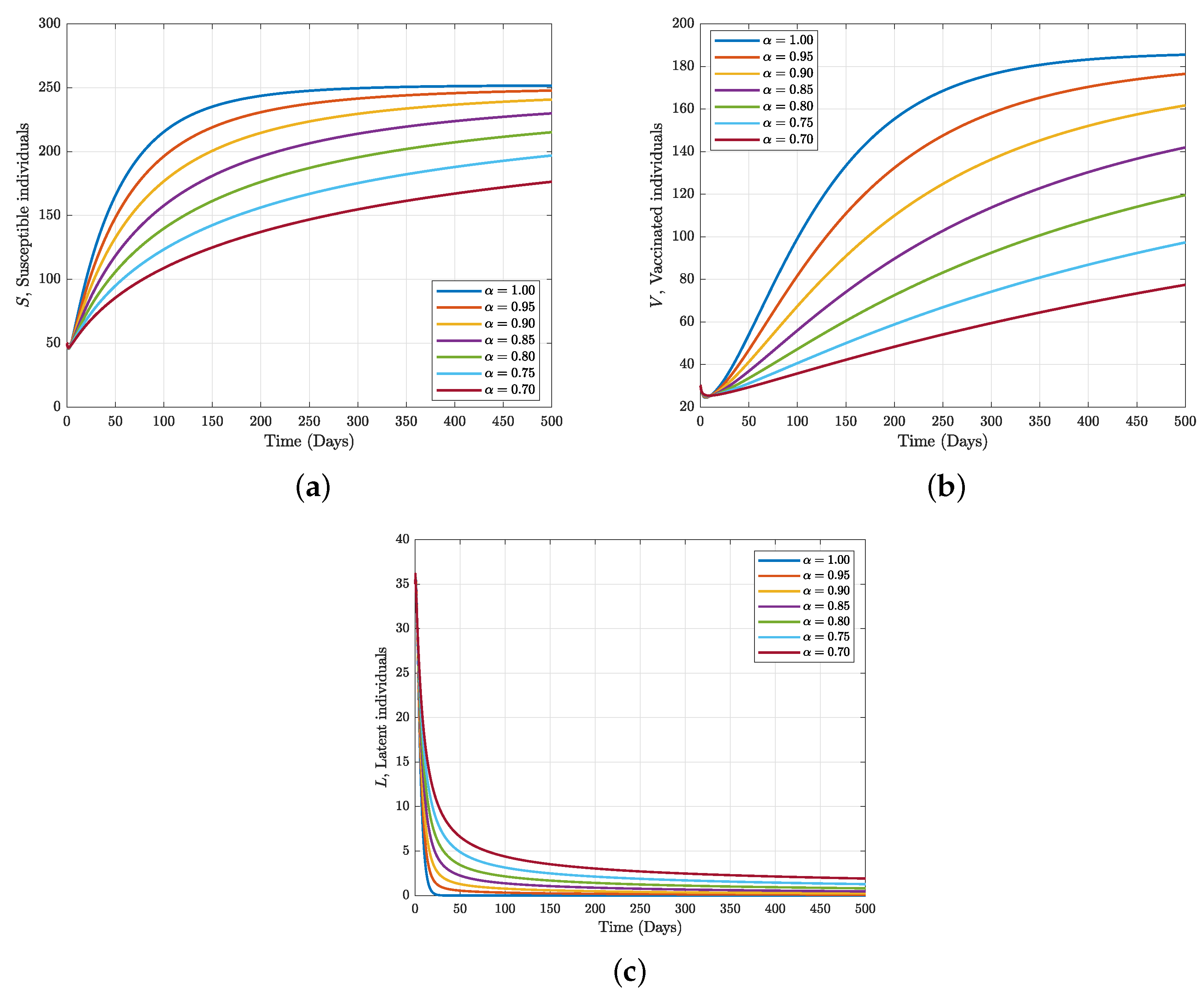
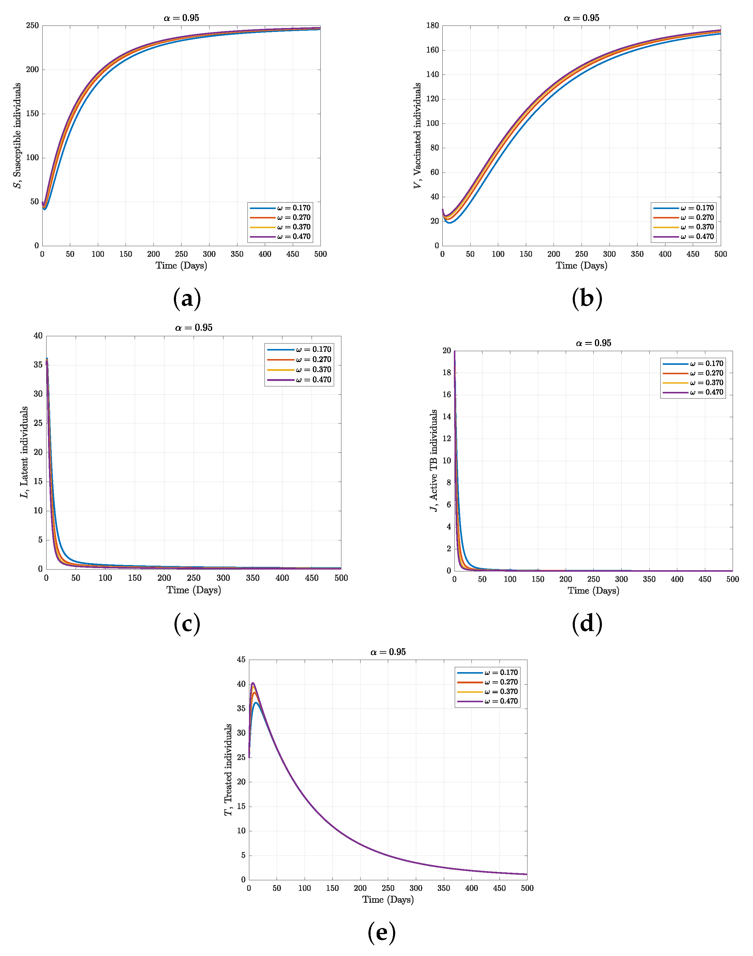
7.3. Numerical Simulation

In this section, we present the numerical algorithms for the Caputo fractional tuberculosis outbreak model, using the famous fractional Adam–Bashforth technique. The parameters used for this simulation can be found in Table 2, and the initial values are S ( 0 ) = 500 , V ( 0 ) = 30 , L ( 0 ) = 35 , J ( 0 ) = 20 , T ( 0 ) = 25 , R ( 0 ) = 20 . For details about this numerical analysis, see [30]. Another numerical method to solve the fractional derivative can also be found in [44]. The formula for the Cauchy problem of the Caputo derivative is
0 C D t α Ψ ( t ) = Υ ( t , Ψ ( t ) ) , u ( 0 ) = u 0 .
With the help of the Caputo integral, (19) can be transformed into
Ψ t Ψ 0 = 1 Γ ( α ) 0 t Υ ( θ , u ( θ ) ) ( t θ ) α 1 d θ .
At the points t ψ + 1 = ( ψ + 1 ) h and t ψ = ψ h , ψ = 0 , 1 , 2 , 3 , 4 , . . . with h being the time step, Equation (20) can be formulated as:
Ψ t ψ + 1 Ψ 0 = 1 Γ ( α ) 0 t ψ + 1 Υ ( θ , Ψ ( θ ) ) ( t ψ + 1 θ ) α 1 d θ .
To integrate (21), refs. [23,33] have applied two-step Lagrange interpolation to solve this integration, and we use similar knowledge to write our proposed model (1) in the following form as [20]:
S ψ + 1 = S 0 + h α Γ ( α + 2 ) φ = 0 ψ Υ ( t φ , S φ ) ( ψ φ + 1 ) α ( ψ φ + 2 + α ) ( ψ φ ) α ( ψ φ + 2 + 2 α ) h α Γ ( α + 2 ) φ = 0 ψ Υ ( t φ 1 , S φ 1 ) ( ψ φ + 1 ) α + 1 ( ψ φ ) α ( ψ φ + 1 + α ) , V ψ + 1 = V 0 + h α Γ ( α + 2 ) φ = 0 ψ Υ ( t φ , V φ ) ( ψ φ + 1 ) α ( ψ φ + 2 + α ) ( ψ φ ) α ( ψ φ + 2 + 2 α ) h α Γ ( α + 2 ) φ = 0 ψ Υ ( t φ 1 , V φ 1 ) ( ψ φ + 1 ) α + 1 ( ψ φ ) α ( ψ φ + 1 + α ) , L ψ + 1 = L 0 + h α Γ ( α + 2 ) φ = 0 ψ Υ ( t φ , L φ ) ( ψ φ + 1 ) α ( ψ φ + 2 + α ) ( ψ φ ) α ( ψ φ + 2 + 2 α ) h α Γ ( α + 2 ) φ = 0 ψ Υ ( t φ 1 , L φ 1 ) ( ψ φ + 1 ) α + 1 ( ψ φ ) α ( ψ φ + 1 + α ) , J ψ + 1 = J 0 + h α Γ ( α + 2 ) φ = 0 ψ Υ ( t φ , J φ ) ( ψ φ + 1 ) α ( ψ φ + 2 + α ) ( ψ φ ) α ( ψ φ + 2 + 2 α ) h α Γ ( α + 2 ) φ = 0 ψ Υ ( t φ 1 , J φ 1 ) ( ψ φ + 1 ) α + 1 ( ψ φ ) α ( ψ φ + 1 + α ) , T ψ + 1 = T 0 + h α Γ ( α + 2 ) φ = 0 ψ Υ ( t φ , T φ ) ( ψ φ + 1 ) α ( ψ φ + 2 + α ) ( ψ φ ) α ( ψ φ + 2 + 2 α ) h α Γ ( α + 2 ) φ = 0 ψ Υ ( t φ 1 , T φ 1 ) ( ψ φ + 1 ) α + 1 ( ψ φ ) α ( ψ φ + 1 + α ) , R ψ + 1 = R 0 + h α Γ ( α + 2 ) φ = 0 ψ Υ ( t φ , R φ ) ( ψ φ + 1 ) α ( ψ φ + 2 + α ) ( ψ φ ) α ( ψ φ + 2 + 2 α ) h α Γ ( α + 2 ) φ = 0 ψ Υ ( t φ 1 , R φ 1 ) ( ψ φ + 1 ) α + 1 ( ψ φ ) α ( ψ φ + 1 + α ) ,

8. Discussion and Conclusions

The computational results of the assessment of our suggested Caputo fractional-order model’s Equation (2) deterministic trajectory in the population are displayed in Figure 4 and Figure 5 while keeping all process parameters. We depict a predetermined pattern by integrating all of the compartments of the framework to achieve determinism figures. In deterministic situations, addressing the population’s contaminated individuals using the rate τ decreases the infectious individuals and increases the population of those who take medication for a set of amount of time. Nonetheless, the system’s Equation (2) dynamics of the curves show realistic behaviour in relation to the mathematical model. According Figure 4a,b, it is easy to see that the compartments start decreasing by decreasing the fractional values, and this shows that physical processes are better explained using the fractional-order derivatives. The operator captured low susceptibility. The biological meaning of this dynamism of Figure 4a–c is that if people have enough knowledge about TB and the rate of the vaccine and its efficacy increase, people will not be exposed to the disease. The dynamics of Figure 4c ensure a low vaccination rate, its low efficacy, and a lack of knowledge about the disease. In Figure 5a–c, compartments start increasing via a decrease in the fractional values. In reality, when we have a large latent or exposed population, this will significantly affect the infected or active TB population. Similarly, the active TB individuals will respond to treatment and recover due to the impact of effective vaccination as a control strategy. In Figure 6 and Figure 7, some of the sensitive parameters are taken to consideration, for example, ω and τ . From Figure 6a,b,e, it is easily to see that the susceptible, vaccination, and treatment compartments increase when the rate of treatment for active TB individuals increases, which clearly indicates that if active TB individuals receive good medication, the proportion of recovered people in the population will increase while the proportion of exposed and infected people in Figure 6c,d will significantly decline. Figure 7a–c, clarify the behaviour of the vaccine rate to TB. It is easily to see that the vaccination compartment increases as the vaccine rate τ increases but not the same as the susceptible and latent classes. This is because when the vaccine works with the rest of the immune system to destroy the pathogen and stop the disease, people who are susceptible move from the susceptible class to the vaccination compartment, which causes a reduction in the latent class. By increasing the vaccine rate τ to TB by 5% (i.e., τ = 0.050 ) as the estimated value, a reduction in the exposed infection is observed. This means that the higher vaccination interaction between the population, the greater the chances of a decrease in the transmission rate to TB, which will lead to elimination of the disease.
There are different phases in an epidemic curve: the exponential phase, the point of inflections, the peaks, and the decompressed peak. These phases exhibit a slow start, a rapid rise, a levelling off, and a decline. Also, these curves can either be concave or convex. The epidemic curve shows that for Figure 2a, there is a sharp decline in the levelling-off of the curve, which looks like a logarithm curve, while Figure 2b shows a rapid rise, a levelling off, and a decline, which looks like an inverted parabolic curve or a concave curve. We were also able to demonstrate similarity between the simulated, real, and fitted data. Figure 2a captures the simulated active TB individuals in Figure 5a. We notice a similarity in the trend of the curve’s behaviour, which means that if the time is extended, it will perfectly correspond to the nature of the real and fitted data.
In this work, we have been able to suggest the Caputo fractional-order model Equation (2) by putting it to the test using the Adams–Bashforth approach, a numerical explicit method with parameter values listed in Table 2. When R 0 > 1 , the DFE point is unstable, and when R 0 < 1 , the DFE point is stable. The sensitivity analysis result was able to suggest to us that increasing the vaccination and treatment rate will help to reduce the spread of the disease. Also, the data fitting result was able to capture to some extent some of the trend in the one year spread of the epidemics in East Africa, most especially in the first month in the year 2020. This study will help public health experts to be able to properly prepare for the pandemic in East Africa. One of the limitations of this work is that the obtained data trend is inconsistent and not fine grain data, which makes it difficult to properly fit the data and affects the nature of the predicted curve. In future work, we suggest that machine learning techniques or different fractional operators or statistical methods could be used to develop this model to mitigate the disease in a different dimension.

Author Contributions

Conceptualisation, O.J.P., K.O., and E.A.; methodology, O.J.P., K.O., E.M., O.B., I.V.N., I.S., U.M.A., and E.A.; software, K.O., E.A., E.M., O.B., and U.M.A.; validation, O.J.P., K.O., and E.A.; formal analysis, K.O., E.M., O.B., I.V.N., I.S., U.M.A., and E.A.; investigation, O.J.P., K.O., and E.A.; resources, K.O. and A.A.; data curation, E.A., O.B., and U.M.A.; writing—original draft preparation, K.O., J.O.A., U.M.A., E.M., I.S., and E.A.; writing—review and editing, E.A. and K.O.; visualisation, E.A., O.B., and U.M.A.; supervision, K.O. and O.J.P.; and project administration, K.O. and O.J.P. All authors have read and agreed to the published version of the manuscript.

Funding

This research received no external funding.

Data Availability Statement

Data used for this research are available on public databases.

Acknowledgments

The authors would like to appreciate Black in Mathematics Association (BMA) for giving us the platform to collaborate as young researchers in order to carry out this work.

Conflicts of Interest

The authors declare no conflict of interest.

References

  1. Tuberculosis Model, a Case Study of Tigania West, Kenya. Available online: https://www.researchgate.net/publication/308631904 (accessed on 2 January 2023).
  2. Molla, K.A.; Reta, M.A.; Ayene, Y.Y. Prevalence of multi drug-resistant tuberculosis in East Africa: A systematic review and meta-analysis. PLoS ONE 2022, 17, e0270272. [Google Scholar] [CrossRef] [PubMed]
  3. Gichuki, J.; Mategula, D. Characterisation of tuberculosis mortality in informal settlements in Nairobi, Kenya: Analysis of data between 2002 and 2016. BMC Infect. Dis. 2021, 21, 718. [Google Scholar] [CrossRef] [PubMed]
  4. Tuberculosis Regional Factsheet. Available online: https://files.aho.afro.who.int/afahobckpcontainer/production/files/iAHO_TB_regional_Factsheet.pdf (accessed on 2 January 2023).
  5. Mnyambwa, N.P.; Philbert, D.; Kimaro, G.; Wandiga, S.; Kirenga, B.; Mmbaga, B.T.; Ngadaya, E. Gaps related to screening and diagnosis of tuberculosis in care cascade in selected health facilities in East Africa countries: A retrospective study. J. Clin. Tuberc. Other Mycobact. Dis. 2021, 25, 100278. [Google Scholar] [CrossRef]
  6. Porous Border Blamed for TB Cases in Kenya and Ethiopia. Available online: https://www.theeastafrican.co.ke/tea/science-health/porous-border-blamed-for-tb-cases-in-kenya-and-ethiopia-3764090 (accessed on 2 January 2023).
  7. Tuberculosis in Kenya. Available online: https://www.tbonline.info/media/uploads/documents/guidelines-on-management-of-leprosy-and-tuberculosis-in-kenya- (accessed on 2 January 2023).
  8. Gakii, G.; Malonza, D. Mathematical Modeling of TB—HIV Co Infection, Case Study of Tigania West Sub County, Kenya. J. Adv. Math. Comput. Sci. 2018, 27, 1–18. [Google Scholar]
  9. Milligan, G.N.; Barrett, A.D. Vaccinology: An Essential Guide; Wiley Blackwell: Chichester, West Sussex, UK, 2015; p. 310. [Google Scholar]
  10. Fine, P.; Eames, K.; Heymann, D.L. Herd Immunity’: A Rough Guide. Clin. Infect. Dis. 2011, 52, 911–916. [Google Scholar] [CrossRef] [PubMed]
  11. Liu, X.; ur Mati, R.; Ahmad, S.; Baleanu, D.; Anjam, Y.N. A new fractional infectious disease model under the non-singular Mittag–Leffler derivative. Waves Random Complex Media 2022, 1–27. [Google Scholar] [CrossRef]
  12. Ahmed, E.; El-Sayed, A.M.A.; El-Saka, H.A. Equilibrium points, stability and numerical solutions of fractional-order predator prey and rabies models. J. Math. Anal. Appl. 2007, 325, 542–553. [Google Scholar] [CrossRef] [Green Version]
  13. Ojo, M.M.; Peter, O.J.; Goufo, E.F.D.; Panigoro, H.S.; Oguntolu, F.A. Mathematical model for control of tuberculosis epidemiology. J. Appl. Math. Comput. 2022, 69, 1865–2085. [Google Scholar] [CrossRef]
  14. Adewale, S.O.; Podder, C.N.; Gumel, A.B. Mathematical analysis of a TB transmission model with DOTS. Can. Appl. Math. Q. 2009, 17, 1–36. [Google Scholar]
  15. Gomes, M.G.M.; Aguas, R.; Lopes, J.S.; Nunes, M.C.; Rebelo, C.; Rodrigues, P.; Struchiner, C.J. How host heterogeneity governs tuberculosis reinfection? Proc. Roy. Soc. B-Biol. Sci. 2012, 279, 2473–2478. [Google Scholar] [CrossRef]
  16. Sterne, J.; Rodrigues, L.; Guedes, I. Does the efficacy of BCG decline with time since vaccination. Int. J. Tuberc. Lung Dis. 2022, 2, 200–207. [Google Scholar]
  17. GHO|By Category|BCG—Immunization Coverage Estimates by Country. Retrieved 25 March 2023. 2023. Available online: https://apps.who.int/gho/data/view.main.80500?lang=en (accessed on 2 April 2023).
  18. Kasereka Kabunga, S.; Doungmo Goufo, E.F.; Ho Tuong, V. Analysis and simulation of a mathematical model of tuberculosis transmission in Democratic Republic of the Congo. Adv. Differ. Equ. 2020, 2020, 642. [Google Scholar] [CrossRef]
  19. Okuonghae, D.; Ikhimwin, B.O. Dynamics of a Mathematical Model for Tuberculosis with Variability in Susceptibility and Disease Progressions Due to Difference in Awareness Level. Front Microbiol. 2016, 2016, 1530. [Google Scholar] [CrossRef] [Green Version]
  20. Nayeem, J.; Sultana, I. Mathematical Analysis of the Transmission Dynamics of Tuberculosis. Am. J. Comput. Math. 2019, 9, 158–173. [Google Scholar] [CrossRef]
  21. Mekonen, K.G.; Balcha, S.F.; Obsu, L.L.; Hassen, A. Mathematical Modeling and Analysis of TB and COVID-19 Coinfection. J. Appl. Math. 2022, 2022, 2449710. [Google Scholar] [CrossRef]
  22. Inayaturohmat, F.; Anggriani, N.; Supriatna, A.K. A mathematical model of tuberculosis and COVID-19 coinfection with the effect of isolation and treatment. Front. Appl. Math. 2022, 8, 2297–4687. [Google Scholar] [CrossRef]
  23. Lee, S.; Park, H.-Y.; Ryu, H.; Kwon, J.-W. Age-Specific Mathematical Model for Tuberculosis Transmission Dynamics in South Korea. Mathematics 2021, 9, 804. [Google Scholar] [CrossRef]
  24. Addai, E.; Adeniji, A.; Peter, O.J.; Agbaje, J.O.; Oshinubi, K. Dynamics of Age-Structure Smoking Models with Government Intervention Coverage under Fractal-fractional-order derivatives. Fractal Fract. 2023, 7, 370. [Google Scholar] [CrossRef]
  25. Almeida, R.A. Caputo fractional derivative of a function with respect to another function. Communic Nonline Sci. Nume. Simul. 2017, 44, 460–481. [Google Scholar] [CrossRef] [Green Version]
  26. Khalil, R.; Horani, M.A.; Yousef, A.; Sababheh, M. A new definition of fractional derivative. J. Comput. Appl. Math. 2014, 264, 65–70. [Google Scholar] [CrossRef]
  27. Scott, A.C. Encyclopedia of Nonlinear Science; Routledge, Taylor and Francis Group: New York, NY, USA, 2005. [Google Scholar]
  28. Sousa, J.; de Oliveira, E.C. A new truncated M-fractional derivative type unifying some fractional derivative types with classical properties. Int. J. Anal. Appl. 2018, 16, 83–96. [Google Scholar]
  29. Jumarie, G. Modified Riemann Liouville derivative and fractional Taylor series of no-differentiable functions further results. Comput. Math. Appl. 2006, 51, 1367–1376. [Google Scholar]
  30. Caputo, M.; Fabrizio, M. A new definition of fractional derivative without singular kernel. Prog. Fract. Differ. Appl. 2015, 1, 73–85. [Google Scholar]
  31. Atangana, A.; Baleanu, D. New fractional derivative without non-local and non-singular kernel: Theory and application to heat transfer model. Therm. Sci. 2016, 20, 763–769. [Google Scholar] [CrossRef] [Green Version]
  32. Zhang, L.; Addai, E.; Ackora-Prah, J.; Dissou Arthur, Y.; Asamoah, J.K.K. Fractional-Order Ebola-Malaria Coinfection Model with a Focus on Detection and Treatment Rate. Comput. Math. Methods Med. 2022, 2022, 6502598. [Google Scholar] [CrossRef]
  33. Ngungu, M.; Addai, E.; Adeniji, A.; Adam, U.M.; Oshinubi, K. Mathematical epidemiological modeling and analysis of monkeypox dynamism with nonpharmaceutical intervention using real data from United Kingdom. Front. Public Health 2023, 11, 1101436. [Google Scholar] [CrossRef]
  34. Addai, E.; Zhang, L.; Preko, A.K.; Asamoah, J.K.K. Fractional order epidemiological model of SARS-CoV-2 dynamism involving Alzheimer’s disease. Healthc. Anal. 2022, 2, 2100114. [Google Scholar] [CrossRef]
  35. Asamoah, J.K.K.; Okyere, E.; Yankson, E.; Opoku, A.A.; Adom-Konadu, A.; Acheampong, E.; Dissou Arthur, Y. Non-fractional and fractional mathematical analysis and simulations for Q fever. Chaos Solitons Fractals 2022, 156, 111821. [Google Scholar] [CrossRef]
  36. Baba, I.A. Existence and uniqueness of a fractional order tuberculosis model. Eur. Phys. J. Plus 2019, 134, 489. [Google Scholar] [CrossRef]
  37. Higazy, M.; Alyami, M.A. New Caputo–Fabrizio fractional order SEIASqEqHR model for COVID-19 epidemic transmission with genetic algorithm based control strategy. Alex. Eng. J. 2020, 59, 4719–4736. [Google Scholar] [CrossRef]
  38. Owolabi, K.M.; Atangana, A. Mathematical modelling and analysis of fractional epidemic models using derivative with exponential kernel. In Fractional Calculus in Medical and Health Science; CRC Press: Boca Raton, FL, USA, 2020; pp. 109–128. [Google Scholar]
  39. Djida, J.D.; Atangana, A. More generalized groundwater model with space-time Caputo Fabrizio fractional differentiation. Numer. Methods Partial Differ. Equ. 2017, 33, 1616–1627. [Google Scholar] [CrossRef] [Green Version]
  40. Singh, J.; Kumar, D.; Qurashi, M.A.; Baleanu, D. A new fractional model for giving up smoking dynamics. Adv. Differ. Equ. 2017, 2017, 88. [Google Scholar] [CrossRef] [Green Version]
  41. Ain, Q.T.; Anjum, N.; Din, A.; Zeb, A.; Djilali, S.; Khan, Z.A. On the analysis of Caputo fractional order dynamics of Middle East Lungs Coronavirus (MERS-CoV) model. Alex. Eng. J. 2022, 61, 5123–5131. [Google Scholar] [CrossRef]
  42. Mustapha, U.T.; Qureshi, S.; Yusuf, A.; Hincal, E. Fractional modeling for the spread of Hookworm infection under Caputo operator. Chaos Solitons Fractals 2020, 137, 109878. [Google Scholar] [CrossRef]
  43. Ahmed, I.; Baba, I.A.; Yusuf, A.; Kumam, P.; Kumam, W. Analysis of Caputo fractional-order model for COVID-19 with lockdown. Adv. Differ. Equ. 2020, 2020, 394. [Google Scholar] [CrossRef]
  44. Mahatekar, Y.; Scindia, P.S.; Kumar, P. A new numerical method to solve fractional differential equations in terms of Caputo–Fabrizio derivatives. Phys. Scr. 2023, 98, 024001. [Google Scholar] [CrossRef]
Figure 1. Pictorial diagram of the model.
Computation 11 00143 g001
Figure 2. Model fitting for January 2020 TB cases for (a) Uganda and (b) Kenya.
Computation 11 00143 g002
Figure 3. The sensitivity analysis of R 0 .
Computation 11 00143 g003
Figure 4. Numerical tuberculosis trajectory for susceptible, vaccinated, and latent individuals under Caputo operator with different fractional order, α .
Computation 11 00143 g004
Figure 5. Numerical tuberculosis trajectory for active TB, treated, and recovered individuals under Caputo operator with a different fractional order, α .
Computation 11 00143 g005
Figure 6. Fractional dynamics for susceptible, vaccinated, and latent individuals when one varies active TB treatment rate with fractional order α = 0.95 .
Computation 11 00143 g006
Figure 7. Fractional dynamics for active TB, treated, and recovered individuals when one varies vaccine rate with fractional order α = 0.95.
Computation 11 00143 g007
Table 1. Description of variables and parameter.
VariablesDescription
S ( t ) Susceptible individuals
V ( t ) Vaccinated individuals
L ( t ) Latent individuals
J ( t ) Active TB individuals
T ( t ) Treated individuals
R ( t ) Recovered individuals
ParametersDescription
ϕ Recruitment rate of individuals in susceptible classes
τ Vaccine rate
ρ Vaccine wane rate
ξ Contact rate
β Efficacy of the vaccine
μ Natural death rate
δ Diseases induced death rate
ε Progression rate from latent to active TB
θ Treatment failure rate
σ Movement rate of individuals in the treated class
γ Recovery rate of treated individuals
ω Rate of treatment for active TB individuals
Table 2. Parameter values in the model (Uganda).
ParametersValuesReferencesUnits
ϕ 5[13]number of persons
τ 0.1[16]persons vaccinated/N
ρ 0.067, 0.1[13]persons loss of immunity/N
ξ 0.6501fitted1/days 1/persons
β 1.6583fitted1/days 1/persons
μ 1/67.7fitted1/days
δ 0.1[13]1/days
ε 0.00375[13]1/days 1/persons
θ 0–1[14,15]1/days 1/persons
σ 0–1assumed1/days 1/persons
γ 0.01[13]1/days
ω 0.1[13]1/days
Table 3. The sensitivity index of R 0 .
ParametersSensitivity Index
ξ 1
ε 0.7975
ϕ 1
ρ 0.0729
μ −1.8502
τ −0.0889
β −0.1977
δ −0.4656
ω −0.4656
Disclaimer/Publisher’s Note: The statements, opinions and data contained in all publications are solely those of the individual author(s) and contributor(s) and not of MDPI and/or the editor(s). MDPI and/or the editor(s) disclaim responsibility for any injury to people or property resulting from any ideas, methods, instructions or products referred to in the content.

