Three-Dimensional Prescribed Performance Tracking Control of UUV via PMPC and RBFNN-FTTSMC

Abstract

To address the search-and-docking problem in multi-stage prescribed performance switching (MPPS) scenarios, this paper presents a novel compound control method for three-dimensional (3D) underwater trajectory tracking control of unmanned underwater vehicles (UUVs) subjected to unknown disturbances. The proposed control framework can be divided into two parts: kinematics control and dynamics control. In the kinematics control loop, a novel parallel model predictive control (PMPC) law is proposed, which is composed of a soft-constrained model predictive controller (SMPC) and hard-constrained model predictive controller (HMPC), and utilizes a weight allocator to enable switching between soft and hard constraints based on task goals, thus achieving global optimal control in MPPS scenarios. In the dynamics control loop, a finite-time terminal sliding mode control (FTTSMC) method combining a finite-time radial basis function neural network adaptive disturbance observer (RBFNN-FTTSMC) is proposed to achieve disturbance estimation and fast convergence of velocity tracking errors. The simulation results demonstrate that the proposed PMPC-FTTSMC approach achieved an average improvement of 33% and 80% in the number of iterations compared with MPC with sliding mode control (MPC-SMC) and traditional MPC methods, respectively. Furthermore, the approach improved the speed of response by 35% and 44%, respectively, while accurately achieving disturbance observation and enhancing the system robustness.

1. Introduction

In recent years, unmanned underwater vehicles (UUVs) have been receiving a significant amount of attention from academia and industry due to their great potential in underwater warning [1], hydrographic surveys [2,3], deep sea exploration [4], and water quality monitoring [5], etc. Using UUVs can significantly reduce the risk to human divers, increase the efficiency and accuracy of data collection, and expand the scope of underwater exploration.

To make UUVs perform complex tasks, underwater trajectory tracking control is essential, which has attracted widespread attention in the field of control engineering. For the motion control of UUVs, tracking the preset desired waypoint for navigation is an essential and critical function [6,7]. However, it is challenging to design reliable tracking controllers due to the nonlinearities in UUV dynamics and the uncertainties in the ocean environment [8,9]. Over the past several decades, various advanced approaches have been proposed to achieve precise position control performance, such as proportional–integral–derivative (PID) control [10], backstepping control (BSC) [11], fuzzy logic control (FLC) [12,13], sliding mode control (SMC) [14,15], adaptive control [16,17], model predictive control (MPC) [18], and disturbance-observer-based feedback control [19,20].

Despite the numerous control approaches that have been proposed, it is still a challenge to achieve optimal control performance in the face of varying ocean environments. Traditional control methods such as PID and BSC may not be suitable in the presence of large disturbances, while FLC and SMC may be more robust; however, FLC requires prior knowledge to formulate fuzzy rules that are often subjective [21]. The SMC method may cause a kind of undesirable high-frequency oscillation on the sliding mode surface, which is called “chattering” because of modeling errors, external disturbances, and discretization [22]. On the other hand, adaptive control and MPC have been shown to have promising results, but adaptive control requires complex modeling and tuning procedures and MPC often involves a long iterative computation time.

To overcome these challenges, researchers have been exploring the use of hybrid control schemes that combine the strengths of different control methods. These hybrid control schemes aim to achieve a better performance, higher accuracy, and improved robustness compared with individual control methods by leveraging the advantages of each method and compensating for their limitations. For example, a global finite-time control method using PID-SMC was proposed to enhance the trajectory tracking performance under model parameter variations and unknown ocean currents [23]. Ref. [24] proposed a linear model predictive control (LMPC) method with a fuzzy logic controller for constrained path following of median and paired fin-propelled robotic fish. In [25], an adaptive fuzzy PID guidance control method was designed, where the control parameters were adjusted by an adaptive fuzzy method to achieve good robustness in different underwater environments. In [26], the kinematic part used MPC to generate a bounded velocity control signal, while the dynamic part used SMC to solve the speed jump problem caused by thruster failure and reduce the computation burden. However, integrating different control methods may introduce new sources of instability or performance degradation, such as constraint violation problems in MPC.

In the context of unpredictable environmental disturbances caused by winds, waves, and ocean currents, the use of disturbance observers plays a crucial role in reconstructing external uncertain information [27]. Ref. [28] proposed an extended state observer (ESO) to estimate the system state information and external disturbances. However, ESO relies on an accurate mathematical model of the system dynamics, and any discrepancies between the actual system and the model can lead to estimation errors. In addition to the steady-state performance, the transient performance also plays a crucial role in task execution. Ref. [29] designed a finite-time disturbance observer to accurately estimate the external disturbances affecting the system. Ref. [30] proposed a synchronization control algorithm based on uncertainty and disturbance estimation (UDE) to achieve rapid and precise synchronization motion. Unlike traditional disturbance observers, which aim for asymptotic convergence, finite-time convergence observers offer the advantage of achieving convergence within a finite time interval. This is particularly important in scenarios where fast and precise disturbance estimation is required.

Prescribed performance tracking control has become a recent research hotspot due to its numerous advantages and applications in UUVs [31]. One of the main reasons for the growing popularity of the prescribed performance tracking control is its ability to provide an improved system performance compared with traditional tracking control methods. It is designed to achieve a desired level of performance, such as a specific settling time, overshoot, or steady-state error [32,33]. By considering the prescribed performance criteria, the control system can be designed to meet specific requirements and avoid undesirable behaviors, such as overshoot, oscillations, or instability. In [34], a robust adaptive dynamic surface control (DSC) scheme with a prescribed performance (PP) was designed to keep the trajectory within the desired values for the prescribed tracking performance, and a nonlinear disturbance observer (NDOB) was also proposed to estimate and compensate for external disturbances. In [35], an error transformation function was proposed to transform the constrained tracking control of the original vessel into an unconstrained system, and stable adaptive neural network control was presented to ensure prescribed tracking performances.

However, less research has been conducted on applying prescribed performance control to address system constraints, thrust limits, and safe operating areas. In this research area, MPC possesses several advantages. MPC utilizes the model of the system to make predictions and optimize control actions over a finite time horizon. It involves repeatedly solving an optimization problem to generate the optimal control sequence based on current system states and predicted future behavior [36]. One of the key advantages of using MPC for prescribed performance control is the ability to formulate and solve the performance specification problem as a constraint in the optimization problem. This means that the controller can explicitly incorporate the desired performance into the control law, ensuring that the system achieves the prescribed performance in a finite time. For example, in [37], the control input and increments were considered and optimized to prescribe the trajectory tracking performance. However, some of the constraints, especially the roll and pitch angle constraints, have rarely been considered. This can be problematic for underwater operations with specific attitude requirements, such as the docking process. In [38], a novel control framework based on MPC with dual closed-loop was designed to improve the tracking performance of constrained UUVs. However, the dynamic control method proposed in this paper cannot guarantee the fast convergence of the velocity tracking error.

Although MPC brings the advantage of achieving the prescribed performance, this advantage comes at price: the heavy computational workload required to solve open-loop optimal control problems. In theoretical studies, the number of iterations required for solving optimal control problems is often omitted, but in engineering practice, it is a critical factor when applying theoretical algorithms to real-world UUVs. Some researchers have recognized this issue and proposed corresponding solutions, such as event-triggered control [39], off-line precomputation [40], and distributed computation schemes [41]. However, the existing study of MPC applied in UUVs mainly focuses on hard constraints, while soft constraints are often omitted or considered less important in the cost function. However, in some cases, soft constraints can also provide benefits such as reducing the number of iterations required for problem-solving, improving the control performance, and reducing the energy consumption of the UUV. Therefore, it is important to investigate the use of soft constraints in the cost function of MPC control algorithms for UUVs and to explore their benefits in practical applications.

To address the problem of a heavy computational burden, and realize the fast convergence of trajectory tracking in MPPS scenarios, a novel control framework that combines MPC guidance law with robust control is proposed to reduce the computational burden. Compared with the traditional MPC guidance law, this paper introduces the method of soft-constrained model predictive control (SMPC) to further reduce the computational complexity and ensure real-time performance. Unlike hard-constrained control, which strictly obeys constraints, SMPC allows for some degree of violation of constraints, while still ensuring that the vehicle’s motion remains within safe and acceptable limits [42]. By incorporating soft constraints and hard constrains, a novel parallel model controller is designed to provide UUVs with greater versatility and robustness, enabling them to complete their missions successfully in challenging conditions. In the dynamics control loop, a finite-time terminal sliding mode control (FTTSMC) method with a finite-time disturbance observer is proposed to reduce the influence of the lumped disturbances and achieve fast convergence. The main contributions can be illustrated as follows:

(1)

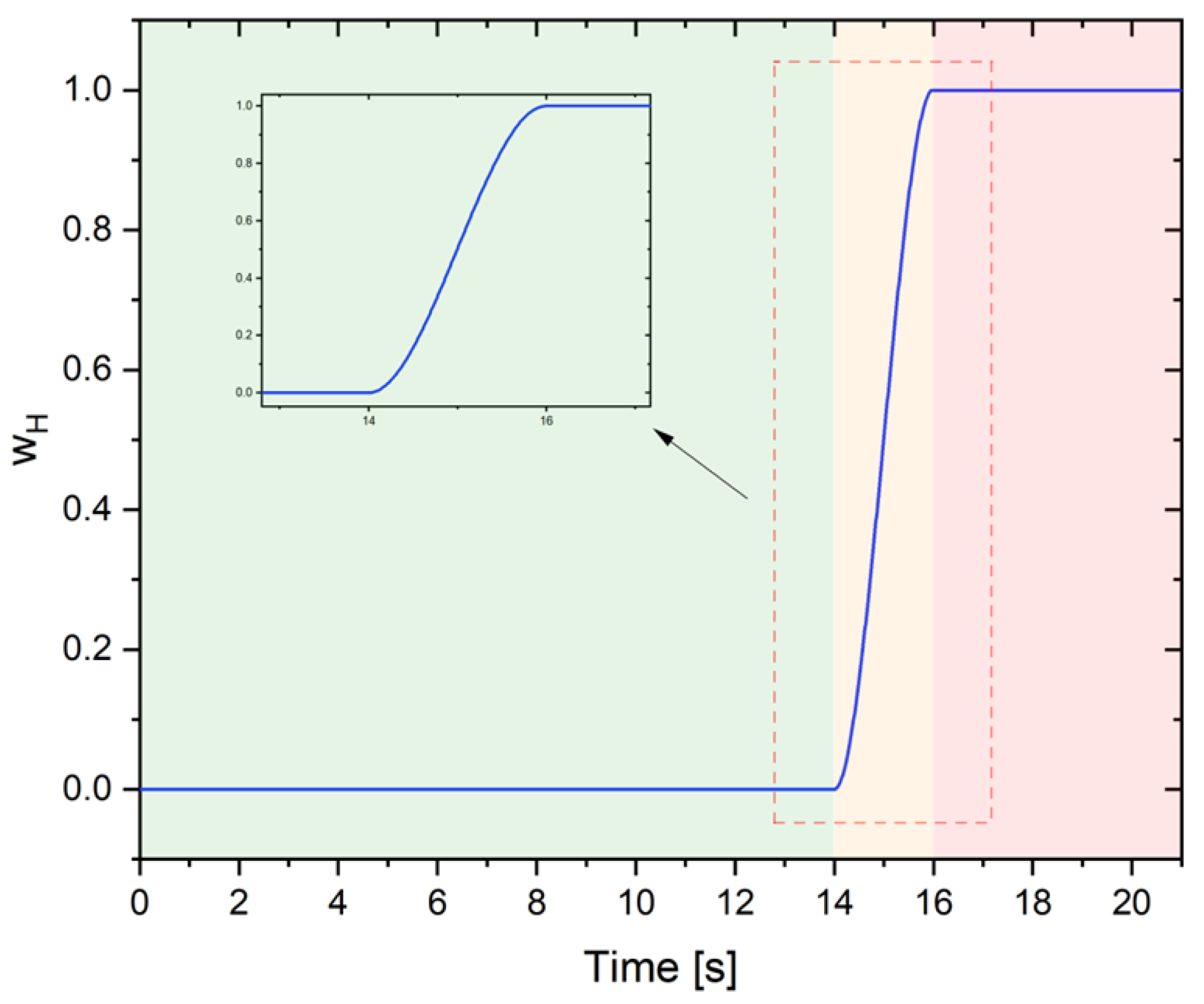
To achieve complex prescribed performance tracking in MPPS scenarios, a novel PMPC guidance law is proposed, which enables the switch between soft and hard constraints in attitude control. This approach utilizes multiple parallel sub-controllers to handle different aspects of the control problem and optimizes the overall control performance. The novelty of the proposed controller lies in its combination of HMPC and SMPC. By integrating HMPC and SMPC, the strengths of both approaches are leveraged in the proposed controller. The inherent ability of HMPC to handle hard constraints ensures that the safety and critical requirements are met, while the incorporation of soft constraints through SMPC offers increased maneuverability and adaptability.

(2)

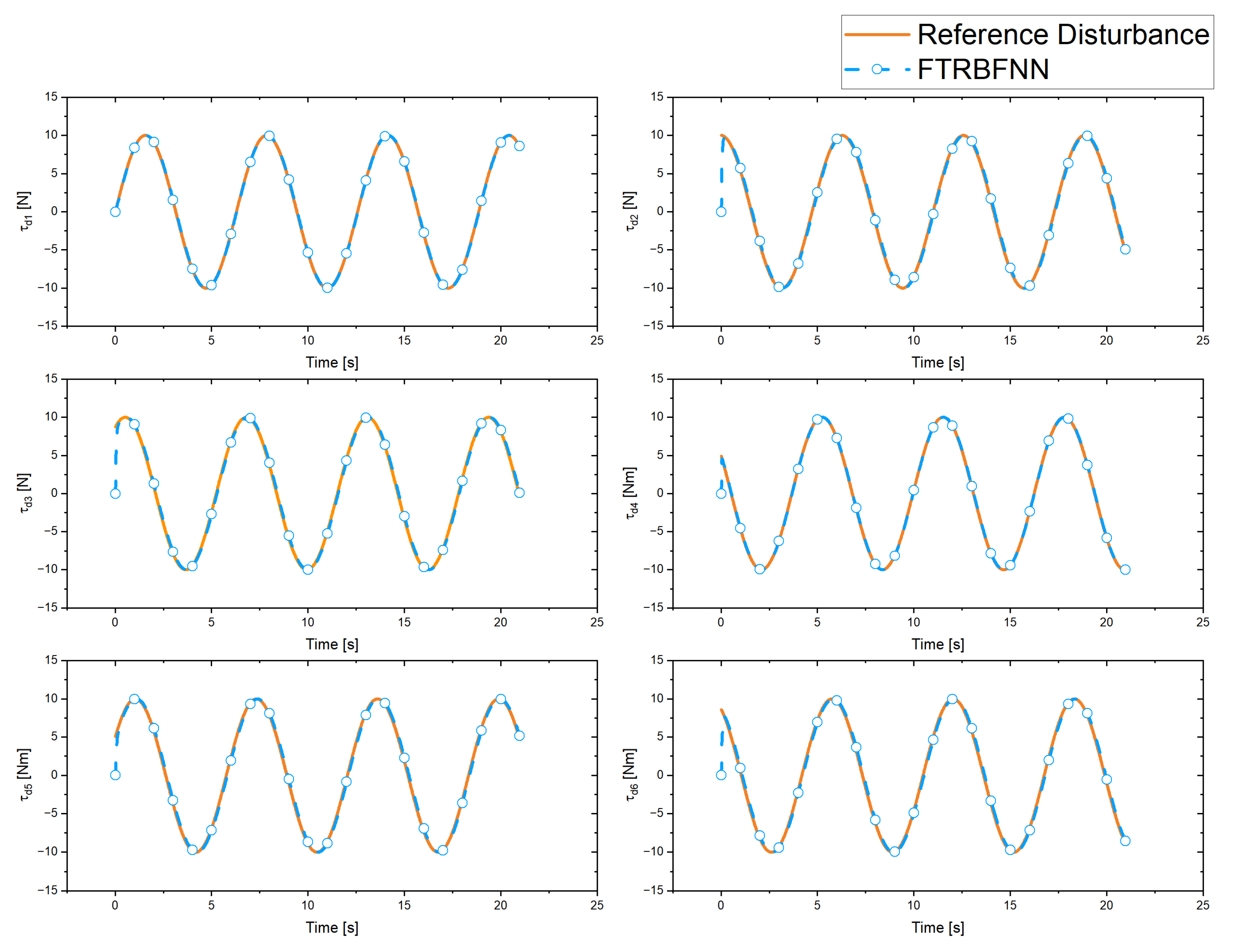
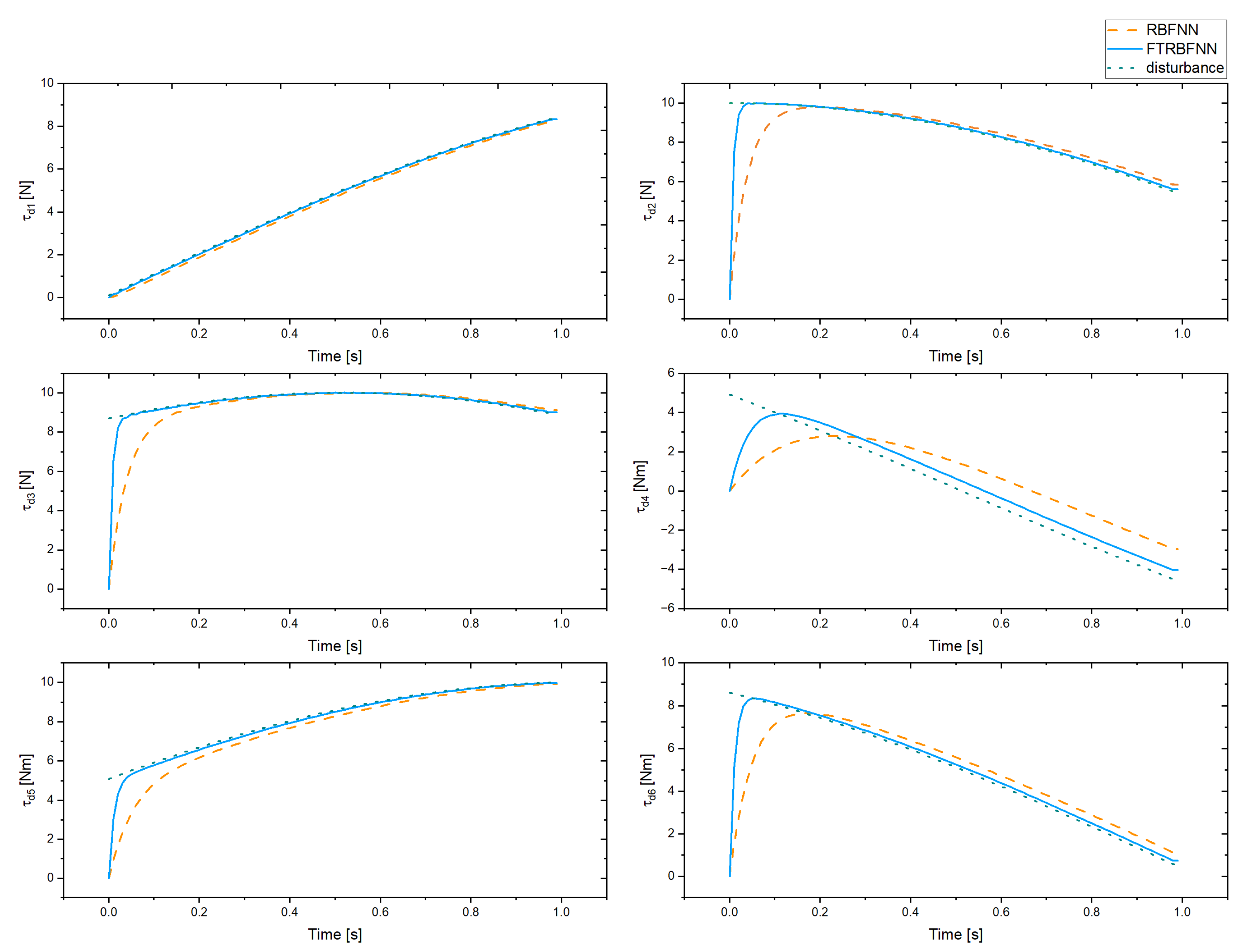
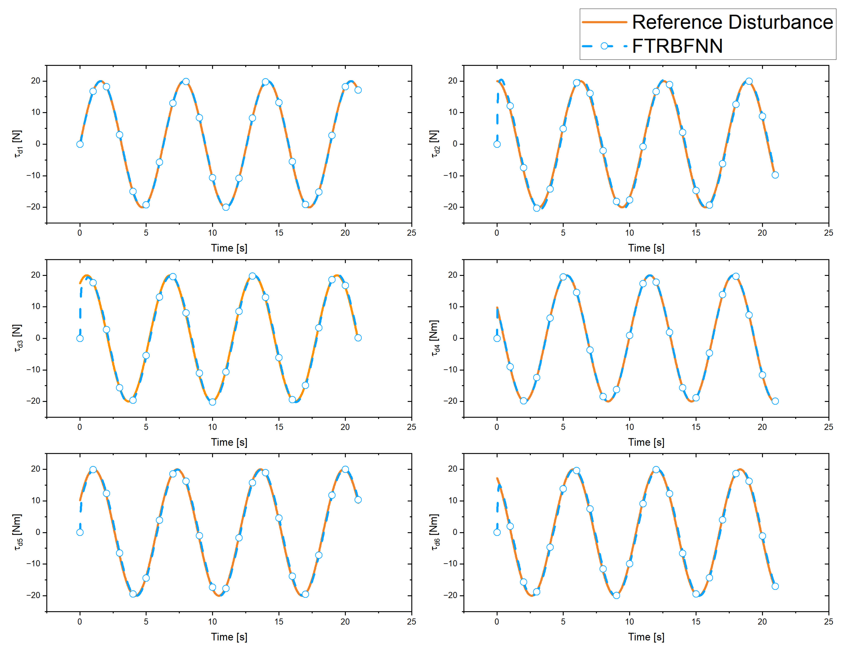
Compared with the robust control based on traditional disturbance observers [43], the RBFNN-FTTSMC method enables fast disturbance estimation and finite-time convergence. This approach combines finite time radial basis function neural network disturbance observer (FTRBFDO) with the finite time terminal sliding mode control to achieve a more accurate and stable disturbance estimation. It can quickly estimate disturbances in real time, improving the overall tracking performance.

(3)

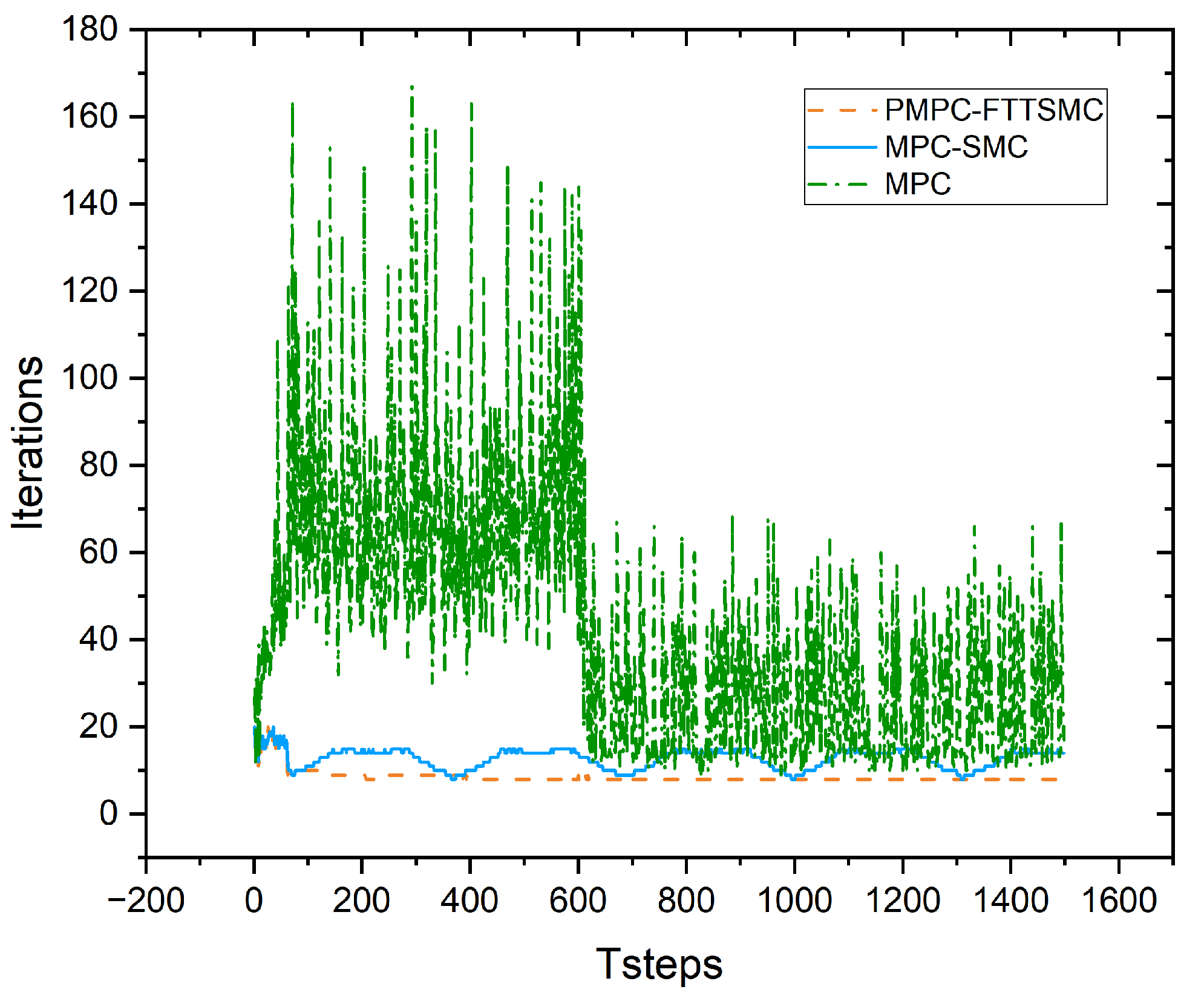
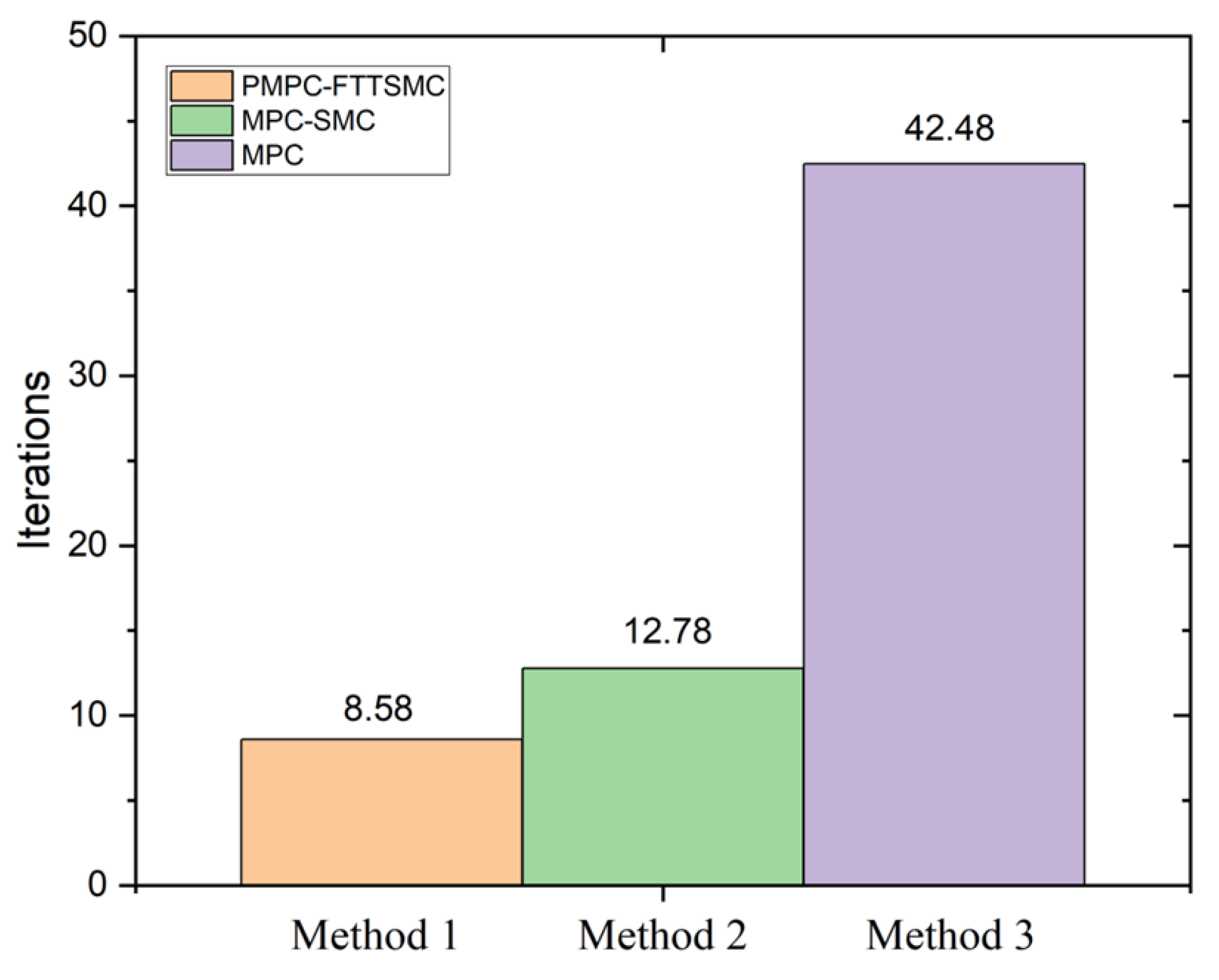
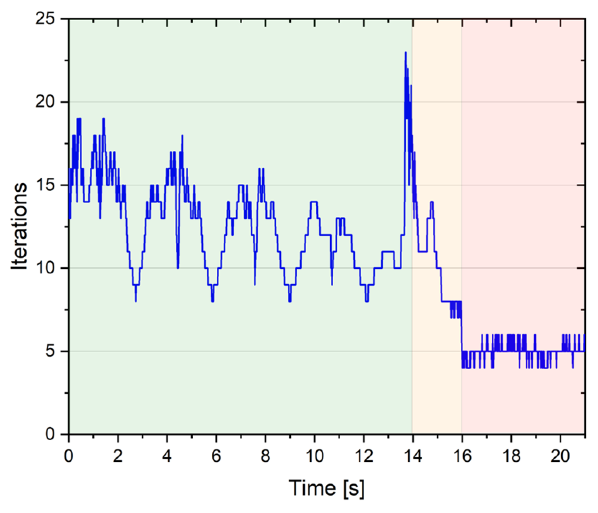
Compared with the traditional MPC method, the proposed integration of PMPC and FTTSMC framework effectively addresses the issue of excessive iteration in traditional MPC, saving the required optimization time. Compared with traditional hybrid control schemes that combine MPC and robust control, the proposed method also solves the problem of constraint violation by using a finite time controller.

The remainder of this paper is organized as follows. Section 2 presents models of the UUV, and formulates the trajectory tracking control problem and search-and-docking mission. In Section 3, a compound control method called PMPC-FTTSMC is proposed for three-dimensional underwater trajectory tracking in MPPS scenarios, which includes PMPC guidance law for kinematics control and FTTSMC control law based on a finite-time radial basis function neural network adaptive disturbance observer for dynamics control. Section 4 provides comparative simulation results with different controllers and the simulation of the mission execution. Section 5 demonstrates the conclusions of this work.

2. Modeling and Problem Formulation

This section introduces the dynamic and kinematic modeling of UUVs and explores the various external disturbances that affect their performance. An overview of the complex three-dimensional underwater search-and-docking mission is also provided in this section.

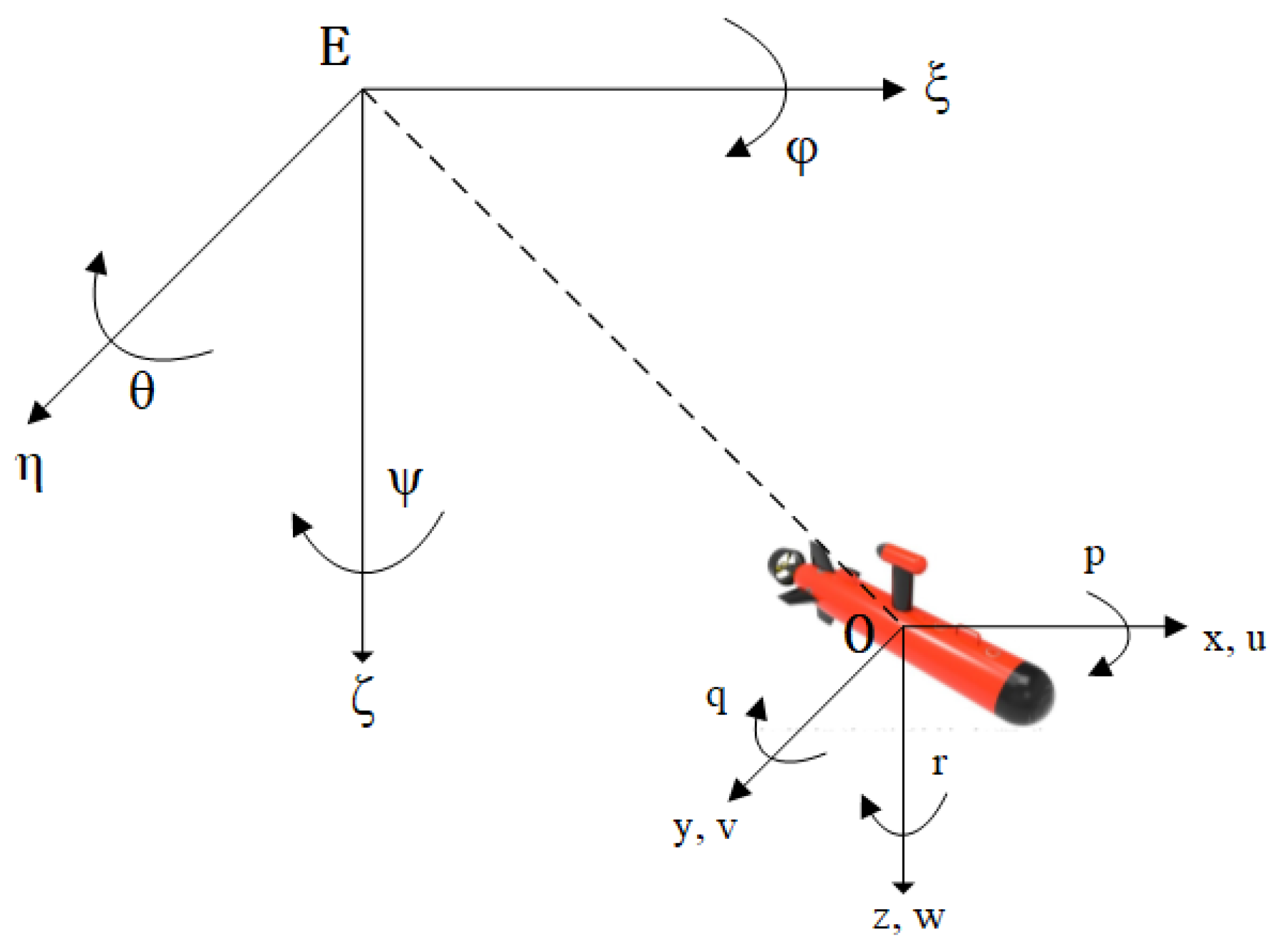
2.1. Frames of Reference

In order to analyze the motion of UUV, as depicted in Figure 1, it is necessary to establish a coordinate system of the UUV first. This coordinate system includes the definition of both an inertial reference frame (I-frame) and a body-fixed frame (B-frame). The origin of the inertial coordinate system is located at the ocean’s surface, while the vehicle coordinate system is fixed at the center of the UUV’s gravity.

2.2. UUV Model

The six degrees of freedom (DOF) motion equations [44] are described as follows:

$$\dot{\eta }=J(\eta )v$$

(1)

$$M\dot{v}+C(v)v+D(v)v=\tau +{\tau }_d$$

(2)

Equation (1) describes the vehicle kinematic model, where the posture vector is given by $\eta ={\left[{\eta }_{\mathrm{x}},{\eta }_{\mathrm{y}},{\eta }_{\mathrm{z}},\varphi ,\theta ,\psi \right]}^{\top }$ in the inertial coordinate system $E-\xi \eta \zeta$. Among them, ${\eta }_{\mathrm{x}},{\eta }_{\mathrm{y}},{\eta }_{\mathrm{z}}$ represents the current position of the UUV, $\varphi$ is the roll angle, $\theta$ is the pitch angle, and $\psi$ is the yaw angle. The velocity vector is given by $v={\left[v_x,v_y,v_z,p,q,r\right]}^{\top }$ in the vehicle coordinate system $O-xyz$. Among them, $v_x,v_y,v_z$ represents the surge speed, sway speed, and heave speed, respectively, and $p,q,r$ represents the roll angular velocity, pitch angular velocity, and yaw angular velocity, respectively. The rotation transformation matrix $J\left(\eta \right)$ is described by the following:

$$J(\eta )=\left[\begin{array}{cc}\begin{array}{c}{J}_1(\eta )\\ O_{3\times 3}\end{array}& \begin{array}{c}{O}_{3\times 3}\\ J_2(\eta )\end{array}\end{array}\right]$$

(3)

$$J_1(\eta )=\left[\begin{array}{ccc}\cos \psi \cos \theta & -\sin \psi \cos \varphi +\cos \psi \sin \theta \sin \varphi & \sin \psi \sin \varphi +\cos \psi \sin \theta \cos \varphi \\ \sin \psi \cos \theta & \cos \psi \cos \varphi +\sin \psi \sin \theta \sin \varphi & -\cos \psi \sin \varphi +\sin \psi \sin \theta \cos \varphi \\ -\sin \theta & \cos \theta \sin \varphi & \cos \theta \cos \varphi \end{array}\right]$$

(4)

$$J_2(\eta )=\left[\begin{array}{ccc}1& \sin \varphi \tan \theta & \cos \varphi \tan \theta \\ 0& \cos \varphi & -\sin \varphi \\ 0& \sin \varphi /\cos \theta & \cos \varphi /\cos \theta \end{array}\right]$$

(5)

where $J_1(\eta )$ is a translational velocity transformation matrix and $J_2(\eta )$ is a rotational velocity transformation matrix.

Equation (2) describes the dynamic model with 6-DOF UUV in B-frame, where $M$ is the system inertia matrix. $C(v)=C_{RB}+C_A$ is the addition matrix of the Coriolis added mass and rigid-body matrix. $D(v)$ is the hydrodynamic damping matrix. $\tau$ is the force and moment acting on the UUV, and ${\tau }_d$ is the unknown oceanic disturbance induced forces and moments. Their forms are as follows:

$$M=diag(m-X_{\dot{u}},m-Y_{\dot{v}},m-Z_{\dot{w}},I_{xx}-K_{\dot{p}},I_{yy}-M_{\dot{q}},I_{zz}-N_{\dot{r}})$$

(6)

$$C_{RB}=\left[\begin{array}{cccc}0& 0& 0& \begin{array}{ccc}0& m{v}_z& -m{v}_y\end{array}\\ 0& 0& 0& \begin{array}{ccc}-m{v}_z& 0& m{v}_x\end{array}\\ 0& 0& 0& \begin{array}{ccc}m{v}_y& -m{v}_x& 0\end{array}\\ \begin{array}{c}0\\ -m{v}_z\\ m{v}_y\end{array}& \begin{array}{c}m{v}_z\\ 0\\ -m{v}_x\end{array}& \begin{array}{c}-m{v}_y\\ m{v}_x\\ 0\end{array}& \begin{array}{ccc}\begin{array}{c}0\\ -I_{zz}r\\ I_{yy}q\end{array}& \begin{array}{c}{I}_{zz}r\\ 0\\ -I_{xx}p\end{array}& \begin{array}{c}-I_{yy}q\\ I_{xx}p\\ 0\end{array}\end{array}\end{array}\right]$$

(7)

$$C_A=\left[\begin{array}{cccccc}0& 0& 0& 0& -Z_{\dot{w}}{v}_z& Y_{\dot{v}}{v}_y\\ 0& 0& 0& Z_{\dot{w}}{v}_z& 0& -X_{\dot{u}}{v}_x\\ 0& 0& 0& -Y_{\dot{v}}{v}_y& X_{\dot{u}}{v}_x& 0\\ 0& -Z_{\dot{w}}{v}_z& Y_{\dot{v}}{v}_y& 0& -N_{\dot{r}}r& M_{\dot{q}}q\\ Z_{\dot{w}}{v}_z& 0& -X_{\dot{u}}{v}_x& N_{\dot{r}}r& 0& -K_{\dot{p}}p\\ -Y_{\dot{v}}{v}_y& X_{\dot{u}}{v}_x& 0& -M_{\dot{q}}q& K_{\dot{p}}p& 0\end{array}\right]$$

(8)

$$\begin{array}{l}D(v)=-diag(X_u+X_{u\left|u\right|}\left|v_x\right|,Y_v+Y_{v\left|v\right|}\left|v_y\right|,Z_w+Z_{w\left|w\right|}\left|v_z\right|,\\ K_p+K_{p\left|p\right|}\left|p\right|,M_q+M_{q\left|q\right|}\left|q\right|,N_r+N_{r\left|r\right|}\left|r\right|)\end{array}$$

(9)

$$\tau ={\left[{\tau }_1,{\tau }_2,{\tau }_3,{\tau }_4,{\tau }_5,{\tau }_6\right]}^{\top }$$

(10)

$${\tau }_d={\left[{\tau }_{d1},{\tau }_{d2},{\tau }_{d3},{\tau }_{d4},{\tau }_{d5},{\tau }_{d6}\right]}^{\top }$$

(11)

where $m$ is the mass of vehicle; $X_{\ast },Y_{\ast },Z_{\ast },K_{\ast },M_{\ast },N_{\ast }$ are measurable hydrodynamic coefficients of UUV, and $I_{xx},I_{yy},I_{zz}$ are the moment of inertia of the vehicle about axis of the body-fixed frame.

Lemma 1

[45]. The equilibrium point  $x=0$ is globally finite-time stable if there exists a Lyapunov function satisfying the following:

$$\dot{V}(x)+{\lambda }_{1}V(x)+{\lambda }_2{V}^k(x)\le 0$$

(12)

where ${\lambda }_1>0,\hspace{0.33em}{\lambda }_2>0,\hspace{0.33em}0<k<1$. The settling time can be given by the following:

$$t\le \frac{1}{{\lambda }_1(1-k)}\ln \frac{{\lambda }_1{V}^{1-k}(x_0)+{\lambda }_2}{{\lambda }_2}$$

(13)

where $V(x_0)$ is the initial value of  $V(x)$

Lemma 2

[46]. (Young’s inequality) For any vectors$a,\hspace{0.33em}b\in R^n$ , the following inequality is true:

$$a^{\top }b\le c^p\frac{{‖a‖}^p}{p}+c^{-q}\frac{{‖b‖}^q}{q}$$

(14)

where $c>0,\hspace{0.33em}p>1,\hspace{0.33em}q>1$, and $(p-1)(q-1)=1$.

Lemma 3

[47]. The radial basis function neural network (RBFNN) system can be applied to approximate a continuous function $f(x)$ by using a linear combination of radial basis functions as activation functions in the following way:

$$f(x)=W^{\top }{\xi }_i(x)+\epsilon (x)$$

(15)

where  $x\in R^n$ is the input vector, $W^{\top }$ is the weight matrix, ${\xi }_i(x)={[{\xi }_1(x),\hspace{0.33em}{\xi }_2(x),\hspace{0.33em}\cdots ,\hspace{0.33em}{\xi }_i(x)\hspace{0.33em}]}^{\top }$ is the Gaussian function vector, and $\epsilon (x)$ is the approximation error that satisfies $\left|\epsilon (x)\right|\le \overline{\epsilon }$ with $\overline{\epsilon }>0$.

Assumption 1.

The buoyancy of the UUV is equal to the gravity, and the center of buoyancy coincides with the center of gravity located at the origin of the vehicle coordinate system.

Assumption 2 

[48]. The unknown disturbances ${\tau }_{d1}$,  ${\tau }_{d2}$,  ${\tau }_{d3}$,  ${\tau }_{d4}$,  ${\tau }_{d5}$, and  ${\tau }_{d6}$ are bounded.

Remark 1.

Assumption 1 simplifies the analysis by assuming ideal conditions, where the UUV’s weight is perfectly balanced by the upward force of buoyancy. However, it is important to acknowledge that in real-world scenarios, factors such as variations in water density and external disturbances may affect the precise alignment of the center of buoyancy and the center of gravity. Therefore, while this assumption serves as a useful starting point for theoretical analysis, it may need to be further refined in some conditions. When the assumption conditions are not met, the model from reference [44] can serve as a viable alternative to adapt to the actual circumstances.

Remark 2.

Assumption 2 refers to the bounded nature of unknown disturbances. Limiting the disturbances within certain bounds is a common practice in control system design and analysis. Nevertheless, the practicality of this assumption depends on the specific application and environmental conditions. Real-world scenarios can involve various unpredictable factors that may lead to disturbances exceeding the assumed bounds. It is advisable to consider the characteristics of the particular system under investigation and to assess the feasibility of this assumption accordingly.

2.3. Problem Formulation

In our research, we propose an effective control strategy for trajectory tracking of the UUV during the docking process. The UUV utilizes an acoustic guidance method for docking. The measurement accuracy of this sensor underwater is dependent on the distance between the sensors on the UUV and the docking station. To ensure the measurement accuracy of the sensor, it is necessary to establish a maximum range for the docking guidance distance, which is referred as the “signal range”. As the mission objectives of the UUV are different in the stages before and after reaching the signal range, it is necessary to define and partition the tasks accordingly.

As illustrated in Figure 2, the search-and-docking mission is divided into three primary phases: search phase, transition phase, and docking phase. During the search phase, the main objective is to swiftly track the desired trajectory. The requirements for the attitude and speed of the UUV are not stringent and are primarily treated as soft constraints. Once the UUV reaches the signal coverage of the docking station, it enters the transition phase. At this phase, the UUV completes the smooth switching from the soft-constrained model predictive control to the hard-constrained model predictive control within the artificially limited time. In the final docking phase, the UUV is subject to strict constraints on attitude, speed, etc., and must accurately dock back to the docking station.

Define the actual state vectors of the UUV as $p_s={\left({\eta }_{\mathrm{x}},{\eta }_y,{\eta }_z\right)}^{\top }$, and define the position vectors of desired moving point as $p_d={\left({\eta }_{\mathrm{xd}},{\eta }_{\mathrm{yd}},{\eta }_{\mathrm{zd}}\right)}^{\top }$. The position tracking error vectors $p_e={\left({\eta }_{xe},{\eta }_{ye},{\eta }_{ze}\right)}^{\top }$ can be calculated by the following:

$$\left\{\begin{array}{c}{\eta }_{xe}={\eta }_x-{\eta }_{xd}\\ {\eta }_{ye}={\eta }_y-{\eta }_{yd}\\ {\eta }_{ze}={\eta }_z-{\eta }_{zd}\end{array}\right.$$

(16)

The vehicle is required to meet three requirements when tracking a desired trajectory in three-dimensional space. Firstly, all of the trajectory tracking error vectors ${\left({\eta }_{xe},{\eta }_{ye},{\eta }_{ze}\right)}^{\top }$ need to converge to zero in a finite time. Then, the constraint switching in the transition phase needs to be completed within the prescribed time $\tilde{T}$. Finally, the attitude vector $(\varphi ,\theta ,\psi )$ needs to satisfy prescribed constraints at different phases of mission execution.

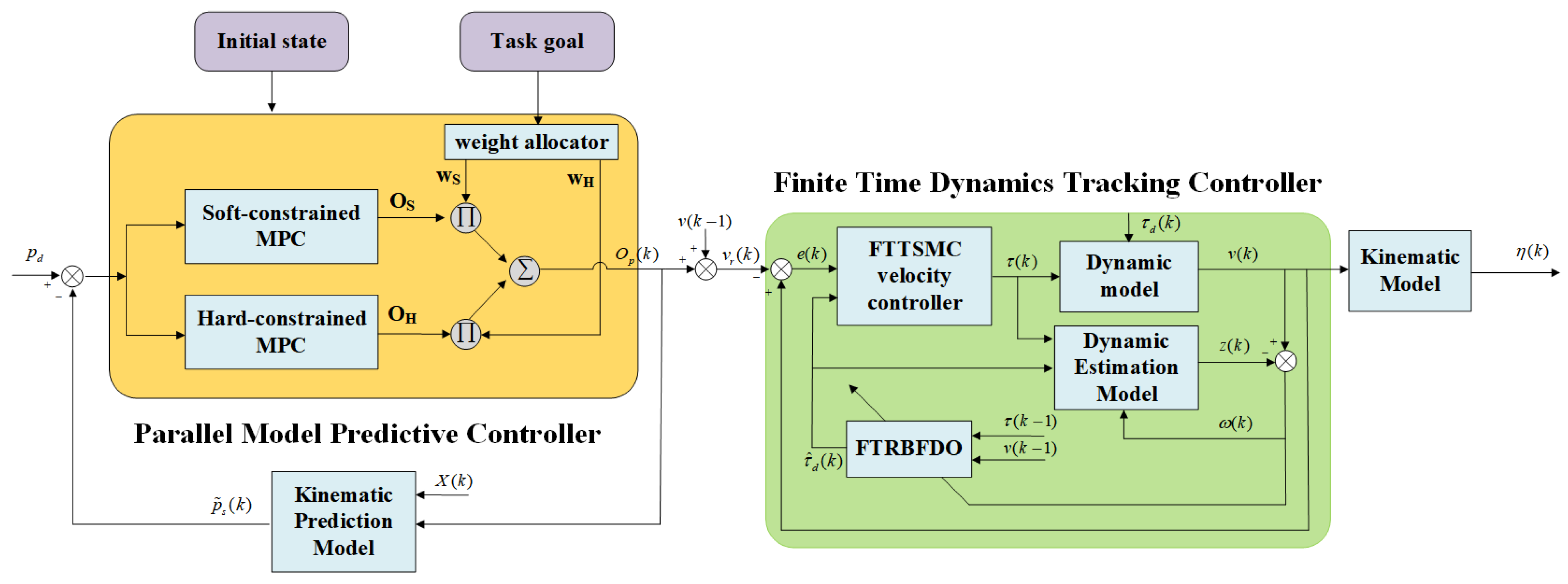
3. Controller Design

As analyzed before, the UUV discussed in this paper is susceptible to unexpected current disturbances. To meet the requirements of three-dimensional trajectory tracking and search-and-docking missions, a compound robust control law has been proposed. This law incorporates parallel model predictive control and finite-time dynamics control, as illustrated in Figure 3.

The proposed trajectory tracking control law is divided into two parts: the kinematics loop and the dynamics loop. The kinematics loop utilizes a parallel model predictive controller with a weight allocator to generate the expected change in velocity $O_p(k)$ for the UUV. By adding this with the real velocity at the previous time step $v(k-1)$, the desired reference velocity at the current time step $v_r(k)$ can be obtained. The dynamics loop implements a finite-time terminal sliding mode controller with FTRBFDO to ensure that the velocity error in six degrees of freedom converges to zero within a finite time.

Compared with conventional trajectory tracking controllers, the proposed controller has greater practical value due to three advantages. Firstly, it can smoothly switch constraints for different missions and can prescribe the constraint switching time. Secondly, the finite-time terminal sliding mode controller and finite-time disturbance observer guarantee fast and robust velocity tracking. Finally, the control framework of PMPC-FTTSMC reduces the number of iterations of the nonlinear solver in the model predictive controller.

3.1. Kinematic Prediction Model

The kinematic model and dynamic model of UUV are both nonlinear. In this paper, the UUV model was linearized and discretized and is redefined in terms of the linear time-invariant (LTI) state–space representation with a sampling period $T$ as follows:

$$\eta (k+1)=\eta (k)+T\cdot J(k)v(k)$$

(17)

where $\eta (k)={\left[{\eta }_x(k),{\eta }_y(k),{\eta }_z(k),\varphi (k),\theta (k),\psi (k)\right]}^{\top },\hspace{0.33em}v(k)={\left[v_x(k),v_y(k),v_z(k),p(k),q(k),r(k)\right]}^{\top }$, $J(k)$ is the rotation matrix $J\left(\eta \right)$ at the $kth$ sampling instant, let $X(k)=\left[\begin{array}{c}\eta (k)\\ v(k-1)\end{array}\right]$ and $u(k)=v(k)-v(k-1)$, the state–space representation with augmented matrix is derived as follows [37]:

$$\left\{\begin{array}{c}X(k+1)=A(k)X(k)+B(k)u(k)\\ Y(k)=CX(k)\end{array}\right.$$

(18)

where $A(k)=\left[\begin{array}{cc}{I}_6& T\cdot J(k)\\ O_{6\times 6}& I_6\end{array}\right]$, $B(k)=\left[\begin{array}{c}T\cdot J(k)\\ I_6\end{array}\right]$, $C=\left[\begin{array}{cc}{I}_3& O_{3\times 9}\end{array}\right]$.

Remark 3.

Equation (18) is derived as follows:

$$\begin{array}{l}X(k+1)=\left[\begin{array}{c}\eta (k+1)\\ v(k)\end{array}\right]=\left[\begin{array}{c}\eta (k)+T\cdot J(k)v(k)\\ v(k)\end{array}\right]\\ =\left[\begin{array}{c}\eta (k)+T\cdot J(k)v(k)+T\cdot J(k)v(k-1)-T\cdot J(k)v(k-1)\\ v(k)+v(k-1)-v(k-1)\end{array}\right]\\ =\left[\begin{array}{c}\eta (k)+T\cdot J(k)v(k-1)\\ v(k-1)\end{array}\right]+\left[\begin{array}{c}T\cdot J(k)v(k)-T\cdot J(k)v(k-1)\\ v(k)-v(k-1)\end{array}\right]\\ =\left[\begin{array}{cc}{I}_6& T\cdot J(k)\\ O_{6\times 6}& I_6\end{array}\right]\left[\begin{array}{c}\eta (k)\\ v(k-1)\end{array}\right]+\left[\begin{array}{c}T\cdot J(k)\\ I_6\end{array}\right]\left[v(k)-v(k-1)\right]\end{array}$$

(19)

According to the state prediction model, given an input sequence $\tilde{u}(k)$, the prediction state sequence $\tilde{X}(k)$ of UUV can be calculated by simulating the model forward over $N_p$ sampling intervals, where $N_p$ is the prediction horizon. The stacked vectors $\tilde{u}(k)$, $\tilde{X}(k)$ are described as follows:

$$\tilde{u}(k)=\left[\begin{array}{c}u(k|k)\\ u(k+1|k)\\ u(k+2|k)\\ \begin{array}{c}⋮\\ u(k+N_p-1|k)\end{array}\end{array}\right] \tilde{X}(k)=\left[\begin{array}{c}X(k+1|k)\\ X(k+2|k)\\ X(k+3|k)\\ \begin{array}{c}⋮\\ X(k+N_p|k)\end{array}\end{array}\right]$$

(20)

where $u(k+i|k)$ and $X(k+i|k)$ are the input vector and state vector at time $k+i$ predicted at time k, respectively. According to Equation (18), $X(k+i|k)$ can be calculated by the following:

$$\begin{array}{l}X(k+i|k)=A(k)X(k+i-1|k)+B(k)u(k+i-1|k)\\ =A{(k)}^{i}X(k|k)+{\displaystyle \sum _{j=0}^{i-1}A{(k)}^{i-1-j}}B(k)u(k+j|k)\end{array}$$

(21)

Thus, the prediction of position sequence ${\tilde{p}}_s(k)$ can be obtained by the following:

$${\tilde{p}}_s(k)=\left[\begin{array}{c}{p}_s(k+1|k)\\ p_s(k+2|k)\\ p_s(k+3|k)\\ \begin{array}{c}⋮\\ p_s(k+N_p|k)\end{array}\end{array}\right]$$

(22)

where $p_s(k+i|k)=C(k)X(k+i|k)$ is the position of UUV at time $k+i$ predicted at sample time $k$.

3.2. Parallel Model Predictive Controller

In this section, based on the kinematic prediction model of UUV, a parallel model predictive controller is designed, so that UUV can find the optimal control law by minimizing the objective function under the constraints in the control domain. PMPC is comprised of a soft-constrained model predictive controller, a hard-constrained model predictive controller (HMPC), and a weight allocator. Define the expected change in velocity $O_p(k)={\left[\Delta u(k),\Delta v(k),\Delta w(k),\Delta p(k),\Delta q(k),\Delta r(k)\right]}^{\top }$. The function of PMPC is defined as follows:

$$O_P(k)=\underset{HMPC}{\underbrace{O_H(k)\cdot w_H(k)}}+\underset{SMPC}{\underbrace{O_S(k)\cdot w_S(k)}}$$

(23)

$$O_H\left(k\right)={\left[\Delta u_H\left(k\right),\Delta v_H\left(k\right),\Delta w_H\left(k\right),\Delta p_H\left(k\right),\Delta q_H\left(k\right),\Delta r_H\left(k\right)\right]}^{\top }$$

(24)

$$O_S(k)={\left[\Delta u_s(k),\Delta v_s(k),\Delta w_s(k),\Delta p_s(k),\Delta q_s(k),\Delta r_s(k)\right]}^{\top }$$

(25)

where $O_H(k)$ and $O_S(k)$ are the outputs of HMPC and SMPC, respectively. $w_H$ and $w_S$, defined by a transition function, are the outputs of the weight allocator.

3.2.1. HMPC

Based on Equation (21), the prediction position and attitude sequence ${\tilde{p}}_s(k)$ is obtained. Based on these predictions, the controller generates a sequence of control inputs that optimize a certain performance criterion while satisfying the system constraints. The first element of the input sequence is applied to the system, and the subsequent sequence is used as the initial value for the next iteration. The process is repeated at each time step.

Define $p_d(k+i)$ as the desired position of UUV at sample time $k$:

$$p_d(k+i)={[{\eta }_{xd}(k+i),{\eta }_{yd}(k+i),{\eta }_{zd}(k+i)]}^{\top }$$

(26)

The cost function of HMPC is defined as follows:

$$\begin{array}{l}{O}_H(k)={\displaystyle \sum _{i=1}^{N_p}\left[{‖p_s(k+i|k)-p_d(k+i)‖}_Q^2\right]}+{\displaystyle \sum _{i=1}^{N_c}{‖u(k+i-1|k)‖}_R^2}\\ s.t.\hspace{1em}\hspace{1em}\hspace{1em} u_{\min } \le u(k+i)\le u_{\max }\\ \hspace{0.33em}\hspace{0.33em}\hspace{0.33em}\hspace{0.33em}\hspace{0.33em}\hspace{0.33em}\hspace{0.33em}\hspace{0.33em}\hspace{0.33em}\hspace{0.33em}\hspace{0.33em}\hspace{0.33em}\hspace{0.33em}\hspace{0.33em}\hspace{0.33em}\hspace{0.33em}{X}_{\min } \le X(k+i)\le X_{\max }\hspace{0.33em}\end{array}$$

(27)

where ${‖x‖}_Q^2=x^{\top }Qx$; $Q$ and $R$ are the weight matrices; $u(k+i-1|k)$ is the system input at time $k+i$ predicted at time $k$; $N_p$ is the predictive horizon, and $N_c$ is the control horizon; $u_{\max }$, $u_{\min }$ represents the requirements for input smoothness, and $X_{\max }$, $X_{\min }$ represents the constraints on attitude, speed, and other states of UUV. Equation (27) is designed to ensure the system tracks the desired trajectory smoothly and quickly.

3.2.2. SMPC

In SMPC, input constraints are hard constraints, while state constraints are softened by the introduction of slack variables. The cost function of SMPC is defined by the following:

$$\begin{array}{l}{O}_S(k)=\underset{\text{path following}}{\underbrace{P_1\cdot d_1}}+\underset{\text{input cost}}{\underbrace{P_2\cdot d_2}}+\underset{\text{attitude cost}}{\underbrace{P_3\cdot (d_3^{+}+d_4^{-})+P_4\cdot (d_5^{+}+d_6^{-})}}\\ s.t.\hspace{0.33em}\hspace{0.33em}\hspace{0.33em}\hspace{0.33em}\hspace{0.33em}\hspace{0.33em}{\displaystyle \sum _{i=1}^{N_p}\left[{‖p_s(k+i|k)-p_d(k+i)‖}_Q^2\right]}-d_1=0\\ \hspace{0.33em}\hspace{0.33em}\hspace{0.33em}\hspace{0.33em}\hspace{0.33em}\hspace{0.33em}\hspace{0.33em}\hspace{0.33em}\hspace{0.33em}{\displaystyle \sum _{i=1}^{N_c}{‖u(k+i-1|k)‖}_R^2}-d_2=0\\ \hspace{0.33em}\hspace{0.33em}\hspace{0.33em}\hspace{0.33em}\hspace{0.33em}\hspace{0.33em}\hspace{0.33em}\hspace{0.33em}\hspace{0.33em}\varphi (k)+d_3^{+}-d_3^{-}={\varphi }_{\max }\hspace{0.33em}\hspace{0.33em}\hspace{0.33em}\hspace{0.33em}\hspace{0.33em}\hspace{0.33em}\hspace{0.33em}\hspace{0.33em}\varphi (k)+d_4^{+}-d_4^{-}={\varphi }_{\min }\\ \hspace{0.33em}\hspace{0.33em}\hspace{0.33em}\hspace{0.33em}\hspace{0.33em}\hspace{0.33em}\hspace{0.33em}\hspace{0.33em}\hspace{0.33em}\theta (k)+d_5^{+}-d_5^{-}={\theta }_{\max }\hspace{0.33em}\hspace{0.33em}\hspace{0.33em}\hspace{0.33em}\hspace{0.33em}\hspace{0.33em}\hspace{0.33em}\theta (k)+d_6^{+}-d_6^{-}={\theta }_{\min }\\ \hspace{0.33em}\hspace{0.33em}\hspace{0.33em}\hspace{0.33em}\hspace{0.33em}\hspace{0.33em}\hspace{0.33em}\hspace{0.33em}\hspace{0.33em}{u}_{\min }\le u(k+i)\le u_{\max }\hspace{0.33em}\hspace{0.33em}\hspace{0.33em}\hspace{0.33em}\hspace{0.33em}\hspace{0.33em}\hspace{0.33em}\hspace{0.33em}\hspace{0.33em}\hspace{0.33em}{d}_i,d_i^{+},d_i^{-}\ge 0\hspace{0.33em}\hspace{0.33em}\hspace{0.33em}\hspace{0.33em}\hspace{0.33em}\end{array}$$

(28)

where $P_i$ is the weight coefficient indicating the priority of the optimization part, and $d_i^{+},d_i^{-}$ are the slack variables.

3.2.3. Weight Allocator

The weight allocator in PMPC is used to adjust the weights of different objectives in the cost function during different phases of operation. It enables the control system to switch between soft and hard constraints based on task goals, and also helps to improve the smoothness and effectiveness of the control approach. In order to achieve a smooth transition in a prescribed time, the transition function is defined as follows:

$$\hspace{0.33em}\hspace{0.33em}\left\{\begin{array}{l}{w}_S(k)=1-w_H(k)\hfill \\ w_H(k)=\left\{\begin{array}{l}0,\hspace{0.33em}\hspace{0.33em}\hspace{0.33em}\hspace{0.33em}\hspace{0.33em}\hspace{0.33em}\hspace{0.33em}\hspace{0.33em}\hspace{0.33em}(k<k_{T1})\hfill \\ 3x^2-2x^3,(k_{T1}<k<k_{T2})\hfill \\ 1,\hspace{0.33em}\hspace{0.33em}\hspace{0.33em}\hspace{0.33em}\hspace{0.33em}\hspace{0.33em}\hspace{0.33em}\hspace{0.33em}\hspace{0.33em}\hspace{0.33em}(k>k_{T2})\hfill \end{array}\right.\hfill \end{array}\right.$$

(29)

where $k_{T1}<k_{T2}$ are the prescribed transition time variables, $T$ is the sampling interval, and $x$ is the temp variable defined as follows:

$$x=\frac{k-k_{T1}}{k_{T2}-k_{T1}}$$

(30)

Thus, the prescribed time $\tilde{T}$ of transition phase can be described by the following:

$$\tilde{T}=T{k}_{T2}-T{k}_{T1}$$

(31)

Remark 4.

The proposed PMPC guidance law provides an efficient way to switch between soft and hard constraints in tracking control by applying a weight allocator that can dynamically assign weights to sub-controllers. This feature is particularly advantageous in MPPS scenarios, where UUVs may have varying objectives at different stages of their mission. Furthermore, the method can overcome infeasibility issues by utilizing soft constraints. The lower-priority constraints can be violated with a certain penalty, providing greater flexibility in achieving the desired control objectives.

3.3. Dynamics Controller Design

3.3.1. Finite-Time RBF Disturbance Observer

External disturbances can introduce uncertainties into the mathematical model, potentially compromising the trajectory tracking performance [49]. To ensure robust dynamics control, it is essential to have fast and precise disturbance estimation. To tackle this challenge, this paper proposes a finite time radial basis function disturbance observer. The FTRBFDO uses a radial basis function neural network to estimate the unknown disturbance. This approach provides fast and accurate disturbance estimation by using the capability of the RBF adaptive algorithm to approximate unknown nonlinear functions. Additionally, the adaptive nature of FTRBFDO ensures that the observer can adapt to changes in the disturbance over time, further improving the accuracy of the disturbance estimate.

Typically, disturbances cannot be directly measured. In order to accurately estimate these disturbances, it is necessary to first establish a dynamic estimation model:

$$\dot{z}=M^{-1}\left[-C(v)v-D(v)+\tau +{\widehat{\tau }}_d(v,\tau |w)\right]+a_0{(v-z)}^m+b_0{(v-z)}^n$$

(32)

where $a_0=diag(a,a,a,a,a,a),\hspace{0.33em}a>0;\hspace{0.33em}$$b_0=diag(b,b,b,b,b,b),\hspace{0.33em}b>0;\hspace{0.33em}$$n>1,\hspace{0.33em}0<m<1;\hspace{0.33em}\hspace{0.33em}$$z(k)={\left[{\widehat{v}}_x(k),{\widehat{v}}_y(k),{\widehat{v}}_z(k),\widehat{p}(k),\widehat{q}(k),\widehat{r}(k)\right]}^{\top };\hspace{0.33em}$ ${\widehat{\tau }}_d(v,\tau |w)={\left[{\widehat{\tau }}_{d1},{\widehat{\tau }}_{d2},{\widehat{\tau }}_{d3},{\widehat{\tau }}_{d4},{\widehat{\tau }}_{d5},{\widehat{\tau }}_{d6}\right]}^{\top }$ is the output of observer, which is described in the following form:

$${\widehat{\tau }}_{di}(v,\tau |w)={\displaystyle \sum _{j=1}^r{w}_{ij}\cdot \exp (-\frac{{‖x_i-c_{ij}‖}^2}{2{\overline{\sigma }}_{ij}^2})}\hspace{0.33em}\hspace{0.33em}\hspace{0.33em}\hspace{0.33em}i=1,2\dots 6$$

(33)

where $x_i=\left[{\tau }_i(k-1),v_i(k-1)\right]$ is the input of observer; $r$ is the number of neurons; $c_{ij}$ is the vector value of the center point and ${\overline{\sigma }}_{ij}$ is the width vector of the Gaussian kernel function of the hidden layer neuron; $w_{ij}$ represents optimal weight of RBF neural network; and $c_{ij}$, ${\overline{\sigma }}_{ij}$ and $w_{ij}$ are updated by the observer error $\omega$, which is defined as follows:

$$\omega (k)=v(k)-z(k)$$

(34)

where $v(k)$ is the velocity vector in Equation (2), $z(k)$ is the estimated velocity vector in Equation (32).

Proposition 1.

If the optimal weight matrix $W$ of RBF neural network is selected as $\dot{W}={\tilde{\mu }}_1(\xi {\omega }^{\top }-{\tilde{\mu }}_{2}W)$ with parameters ${\tilde{\mu }}_1>0$ and${\tilde{\mu }}_2>0$ . The observer error $\omega$ can approach a region around the origin within a finite time.

Proof: 

Please refer to [47]. □

3.3.2. Finite-Time Terminal Slide Mode Controller

As a result of the adoption of the control framework of PMPC-FTTSMC, if the speed cannot be converged in time, it may lead to problems such as constraint violation. To solve the problem, an FTTSMC law [50] is proposed as a solution.

Define the reference velocity $v_r={\left[v_{xr},v_{yr},v_{zr},p_r,q_r,r_r\right]}^{\top }$, and the velocity error vector $e={[e_1,e_2,e_3,e_3,e_4,e_6]}^{\top }$ can be defined as follows:

$$e=v-v_r$$

(35)

Differentiating Equation (35) yields the following:

$$\dot{e}=\dot{v}-{\dot{v}}_r$$

(36)

where ${\dot{v}}_r$ can be obtained by the following:

$${\dot{v}}_r(k)=O_p(k)/T$$

(37)

Furthermore, a terminal sliding mode surface is defined as follows:

$$s_i=e_i+C_{1i}{\displaystyle {\int }_0^t{e}_i}\hspace{0.33em}dt\hspace{0.33em}+C_{2i}{\displaystyle {\int }_0^{t}si{g}^{r_{e_i}}(e_i)}\hspace{0.33em}dt\hspace{0.33em}\hspace{0.33em}\hspace{0.33em}\hspace{0.33em}\hspace{0.33em}i=1,2\dots 6$$

(38)

where $C_{1i}>0,\hspace{0.33em}{C}_{2i}>0,\hspace{0.33em}0<r_{e_i}<1$; $e_i$ represents the $ith$ element of vector $e$, $C_{1i}$ represents $ith$ element of vector $C_1$, $C_{2i}$ represents $ith$ element of vector $C_2$, and $r_{e_i}$ represents $ith$ element of vector $r_e$.

$$\left\{\begin{array}{l}sign(x)=\left\{\begin{array}{c}1,\hspace{0.33em}\hspace{0.33em}\hspace{0.33em}x\ge 0\\ -1,\hspace{0.33em}\hspace{0.33em}x<0\end{array}\right.\\ si{g}^r(x)={\left|x\right|}^{r}sign(x)\end{array}\right.$$

(39)

In discrete form, Equation (38) can be obtained as follows:

$$s_i(k)=e_i(k)+C_{1i}{\displaystyle \sum _{j=1}^k{e}_i(j)}\hspace{0.33em}+C_{2i}{\displaystyle \sum _{j=1}^{k}si{g}^{r_{e_i}}(e_i(j))}\hspace{0.33em}dt\hspace{0.33em}\hspace{0.33em}\hspace{0.33em}\hspace{0.33em}\hspace{0.33em}i=1,2\dots 6$$

(40)

In order to eliminate the velocity error to zero in finite time, the control law is presented as follows:

$$\tau =C(v)v+D(v)v-{\widehat{\tau }}_d+M\cdot ({\dot{v}}_r-\mu )$$

(41)

where $\mu ={[{\mu }_1,{\mu }_2,{\mu }_3,{\mu }_4,{\mu }_5,{\mu }_6]}^{\top }$; ${\widehat{\tau }}_d$ is the estimation of ${\tau }_d$, which can be calculated by Equation (33); ${\mu }_i$ is proposed as follows:

$${\mu }_i=C_1{}_i{e}_i+C_{2i}si{g}^{r_{e_i}}(e_i)+k_{1i}{s}_i+k_{2i}si{g}^{r_{s_i}}(s_i)\hspace{0.33em}\hspace{0.33em}\hspace{0.33em}\hspace{0.33em}\hspace{0.33em}i=1,2\dots 6$$

(42)

where $k_{1i}>0,\hspace{0.33em}{k}_{2i}>0,\hspace{0.33em}0<r_{s_i}<1$; $k_{1i}$ represents $ith$ element of vector $k_1$, $k_{2i}$ represents the $ith$ element of vector $k_2$, and $r_{s_i}$ represents the $ith$ element of vector $r_s$.

3.3.3. Stability Analysis

Proposition 2.

Utilizing the control law $\tau$ presented in Equation (41), the velocity tracking error vector  $e={[e_1,e_2,e_3,e_3,e_4,e_6]}^{\top }$ can converge to zero in finite time.

Proof. 

The analysis process consists of two steps to verify the stability and finite-time convergence of the velocity error: The first step is to prove that the sliding mode can be attained in finite time by the proposed heading control law. The second step is to prove that the tracking error can converge to zero in finite time after entering the sliding mode.

• Step 1: Achieving Sliding Mode in Finite Time

To prove the first step, take $i=1$, consider the following Lyapunov function for dynamic control:

$$V_1=\frac{1}{2}{s}_1^2$$

(43)

Differentiating Equation (38) yields the following:

$${\dot{s}}_1={\dot{e}}_1+C_{11}{e}_1+C_{21}si{g}^{r_{e_1}}(e_1)$$

(44)

According to Equation (2), one can obtain the following:

$${\dot{s}}_1=(-C_1(v)v_1-D_1(v)v_1+{\tau }_1+{\tau }_{d1})/M_1-{\dot{v}}_{r1}+C_{11}{e}_1+C_{21}si{g}^{r_e{}_1}(e_1)$$

(45)

where $M_i$ is the $ith$ element on the diagonal of the matrix. $C_i(v)v_i,D_i(v)v_i$ are the $ith$ row of the original matrix $C(v)v,\hspace{0.33em}D(v)v$.

Differentiating Equation (43) yields the following:

$$\begin{array}{l}{\dot{V}}_1=s_1{\dot{s}}_1\\ \hspace{0.33em}\hspace{0.33em}\hspace{0.33em}=s_1[(-C_1(v)v_1-D_1(v)v_1+{\tau }_1+{\tau }_{d1})/M_1-{\dot{v}}_{r1}+C_{11}{e}_1+C_{21}si{g}^{r_e{}_1}(e_1)]\end{array}$$

(46)

when ${\tau }_1=C_1(v)v_1+D_1(v)v_1-{\widehat{\tau }}_{d1}+M_1\cdot ({\dot{v}}_{r1}-{\mu }_1)$, ${\dot{V}}_1$ can be described by the following:

$$\begin{array}{l}{\dot{V}}_1=s_1[-k_{11}{s}_1-k_{21}si{g}^{r_s{}_1}(s_1)+{\tilde{D}}_1]\\ \hspace{0.33em}\hspace{0.33em}\hspace{0.33em}\hspace{0.33em}\le -k_{11}{s}_1^2-k_{21}{\left|s_1\right|}^{{}^{r_s{}_{1+1}}}+\frac{1}{2\sigma }{s}_1^2+\frac{\sigma }{2}{\tilde{D}}_1^2\\ \hspace{0.33em}\hspace{0.33em}\hspace{0.33em}\hspace{0.33em}=-(k_{11}-\frac{1}{2\sigma })s_1^2-k_{21}{\left|s_1\right|}^{{}^{r_{s1}+1}}+\frac{\sigma }{2}{\tilde{D}}_1^2\\ \hspace{0.33em}\hspace{0.33em}\hspace{0.33em}\hspace{0.33em}=-2(k_{11}-\frac{1}{2\sigma })V_1-2^{\frac{{}^{r_{s1}+1}}{2}}{k}_{21}{V}_1^{\frac{{}^{r_{s1}+1}}{2}}+\frac{\sigma }{2}{\tilde{D}}_1^2\end{array}$$

(47)

where $\sigma$ is a user-defined positive constant and $k_{11}-\frac{1}{2\sigma }>0$; ${\tilde{D}}_1={\tau }_{d1}-{\widehat{\tau }}_{d1}$ is the estimation error and will converge to zero in finite time $t_r$ [47]. Thus, Equation (47) can be further derived as follows:

$$\begin{array}{l}{\dot{V}}_1=-2(k_{11}-\frac{1}{2\sigma })V_1-2^{\frac{{}^{r_{s1}+1}}{2}}{k}_{21}{V}_1^{\frac{{}^{r_{s1}+1}}{2}}\\ \hspace{0.33em}\hspace{0.33em}\hspace{0.33em}\hspace{0.33em}=-{\mathrm{\Gamma }}_1{V}_1-{\mathrm{\Gamma }}_2{V}_1^{\frac{{}^{r_{s1}+1}}{2}}\end{array}$$

(48)

where ${\mathrm{\Gamma }}_1=2(k_{11}-\frac{1}{2\sigma }),\hspace{0.33em}{\mathrm{\Gamma }}_2=2^{\frac{{}^{r_{s1}+1}}{2}}{k}_{21}$.

According to Lemma 1, it can be concluded that the sliding mode surface $s_1$ can converge to zero in finite time $t_1$ by the control law ${\tau }_1.$

$$t_1\le t_r+\frac{1}{{\mathrm{\Gamma }}_1(1-\frac{r_{s1}+1}{2})}\ln \frac{{\mathrm{\Gamma }}_1{V}^{1-\frac{r_{s1}+1}{2}}(0)+{\mathrm{\Gamma }}_2}{{\mathrm{\Gamma }}_2}$$

(49)

• Step 2: Velocity Tracking Error Convergence in Finite Time

It can be proven that velocity tracking error $e_1$ will converge to zero in finite time when the sliding mode surface $s_1$ converges to zero. When $s_1=0$, ${\dot{e}}_1$ can be described by the following:

$${\dot{e}}_1=-C_{11}{e}_1-C_{21}si{g}^{r_{e1}}(e_1)$$

(50)

Consider the following Lyapunov candidate for the sliding mode holding stage:

$$V_2=\frac{1}{2}{e}_1^2$$

(51)

Differentiating Equation (51) yields the following:

$$\begin{array}{l}{\dot{V}}_2=e_1{\dot{e}}_1\\ \hspace{0.33em}\hspace{0.33em}\hspace{0.33em}\hspace{0.33em}=-C_{11}{e}_1^2-C_{21}{\left|e_1\right|}^{r_{e1}+1}\\ \hspace{0.33em}\hspace{0.33em}\hspace{0.33em}\hspace{0.33em}=-2C_{11}{V}_2-2^{\frac{{}^{r_{e1}+1}}{2}}{C}_{21}{V}_2^{{}^{\frac{{}^{r_{e1}+1}}{2}}}\\ \hspace{0.33em}\hspace{0.33em}\hspace{0.33em}\hspace{0.33em}=-{\mathrm{\Gamma }}_3{V}_2-{\mathrm{\Gamma }}_4{V}_2^{{}^{\frac{{}^{r_{e1}+1}}{2}}}\end{array}$$

(52)

where ${\mathrm{\Gamma }}_3=2C_{11},\hspace{0.33em}{\mathrm{\Gamma }}_4=2^{\frac{{}^{r_{e1}+1}}{2}}{C}_{21}$.

According to Lemma 1, it can be proven that the velocity tracking error $e_1$ can converge to zero in finite time $t_2$ by the control law ${\tau }_1$

$$t_2\le t_r+\frac{1}{{\mathrm{\Gamma }}_1(1-\frac{r_{s1}+1}{2})}\ln \frac{{\mathrm{\Gamma }}_1{V}_1{}^{1-\frac{r_{s1}+1}{2}}(0)+{\mathrm{\Gamma }}_2}{{\mathrm{\Gamma }}_2}+\frac{1}{{\mathrm{\Gamma }}_3(1-\frac{r_{s1}+1}{2})}\ln \frac{{\mathrm{\Gamma }}_3{V}_2{}^{1-\frac{r_{s1}+1}{2}}(0)+{\mathrm{\Gamma }}_4}{{\mathrm{\Gamma }}_4}$$

(53)

Similarly, it can be proven that $e_2,e_3,\dots e_6$ converge to zero in finite time when utilizing the control law ${\tau }_2,{\tau }_3,\dots {\tau }_6$. □

Proposition 3.

For the PMPC controller (23), consider the cost function with the constrains (27) (28), utilizing positive definite weight matrices $Q$ and $R$ , predict horizon $N_p$ , and control horizon $N_c$ , and guaranteeing the optimal solution of the cost function exists, the nominal stability of the system can be ensured.

Proof. 

For the HMPC controller, select the optimal cost function $O_H(k)$ as a Lyapunov function $V(k)$. It is found that $V(k+1)\le V(k)$ when selecting positive definite weight matrices $Q$ and $R$, predicting horizon $N_p$, controlling horizon $N_c$, and guaranteeing the optimal solution of the cost function exists [51]. Likewise, the asymptotic stability of the SMPC controller can be proven. As PMPC is a linear combination of HMPC and SMPC, the entire PMPC controller is also asymptotically stable. As the kinematic controller is asymptotically stable, the dynamic controller can ensure that the velocity error converges to zero within a finite time, thereby ensuring the stability of the overall closed-loop system. □

Remark 5.

The proposed FTTSMC method with FTRBFDO provides a fast and accurate approach for disturbance estimation, which is crucial for trajectory tracking in dynamic ocean environments. Additionally, the finite-time control law ensures that the velocity error converges to zero within a finite time, which can enhance the stability and robustness of the overall control system and solve the constraint violation problem in traditional hybrid control schemes that combine MPC and robust control.

Remark 6.

The proposed control framework, which integrates PMPC and FTTSMC, can effectively reduce the number of iterations compared with the traditional MPC method. The reasons are as follows:

Firstly, the complexity of the system being controlled can impact the number of iterations needed for convergence. More complex systems may require more iterations. Therefore, by employing the control framework of PMPC-FTTSMC, the proposed PMPC approach reduces the model complexity by focusing only on the UUV kinematic model. Additionally, a smaller control horizon is selected to further simplify the optimization objective function. These measures are all advantageous for reducing the number of iterations required for computation.

Secondly, the selection of the initial point also has a certain degree of impact on the number of iterations. For the control sequence generated by the solver, the first control sequence is used as the input and the subsequent control sequence is used as the initial value for the next iteration. This method effectively reduces the number of iterations compared to selecting the zero vector as the initial value.

Finally, soft constraints can reduce the number of iterations required by allowing for some flexibility in the solution. In traditional model predictive control, hard constraints are often used to ensure that the system operates within certain limits. However, these hard constraints can lead to infeasible solutions, which require additional iterations to find a feasible solution. By using soft constraints, the optimization problem can be formulated in such a way that it is more likely to find a feasible solution on the first iteration, reducing the total number of iterations required.

3.4. Implementation of the Tracking Control Algorithm

3.4.1. Detailed Implementation Process

The complete PMPC-FTTSMC trajectory tracking control algorithm is summarized in Algorithm 1.

Algorithm 1 Three-dimensional Trajectory Tracking Algorithm.

Input: $X(0)$ (initial state), $Step1$ (search phase), $Step\_pass$ (transition phase), $Step2$ (dock ing phase), $u_{\max },u_{\min }$ (input constrains), $X_{\max },X_{\min }$ (state constrains), $N_p$ (predict horizon), $N_c$ (control horizon) begin:

1. $k$ ← $1$  2. $X(k)$ ←$X(0)$  3. while $k\le Step1+Step\_pass+Step2$ do  4. Calculate ${\tilde{p}}_s(k)$ according to Equations (18)–(22)  5. if $k\le Step1$ then  6. Calculate the output of SMPC $O_s(k)$ utilizing Equation (28)  7. else if $k\le Step1+Step\_pass$ then  8. Calculate the output of SMPC and HMPC according to Equations (27) and (28)  9. Calculate the output of weight allocator utilizing Equation (29)  10. else  11. Calculate the output of HMPC $O_H(k)$ utilizing Equation (27)  12. end if  13. Calculate the output of kinematic controller $O_P(k)$ utilizing Equation (23)  14. Calculate the output of disturbance observer ${\widehat{\tau }}_d(k)$ according to Equation (33)  15. Calculate the terminal sliding mode surface $s(k)$ utilizing Equations (35)–(40)  16. Calculate the desired torque $\tau (k)$ according to Equations (41) and (42)  17. Implement $\tau (k)$ to the UUV  18. $k$ ← $k+1$  19. Update the weight matrix $W$ according to Proposition 1  20. Update the State of UUV $X(k)$  21. end while end

3.4.2. Challenges in Real-World Deployment of Algorithm

Although the proposed method shows promise for addressing the control challenges of UUVs, there are several limitations and practical considerations that need to be addressed for its successful implementation.

Firstly, it is important to note that the modeling process in the study involves certain idealized assumptions. These assumptions may not fully capture all real-world complexities and dynamics of UUV systems. Therefore, during the practical implementation of this method, parameter adjustments based on specific system characteristics and environmental conditions may be necessary. Adapting the method to suit the practical requirements of different UUV platforms and operating scenarios is an essential consideration.

Furthermore, some factors such as sensor and actuator faults, and communication delays are not explicitly taken into account in this study. These aspects are significant challenges in real-world UUV applications. To address these issues and enhance system robustness, future research should explore the integration of fault-tolerant control techniques and consider the impact of time delays to further improve the performance and reliability of the proposed method.

4. Simulation

In this section, a comparative study of numerical simulations is performed to verify the effectiveness and stability of the proposed control method. The simulation parameters and the function of disturbance are presented in Section 4.1, and two cases and their results are displayed in Section 4.2 and Section 4.3. The first is an underwater spiral trail, the other is the trajectory of search-and-docking mission.

4.1. Simulation Preparation

Numerical simulations are carried out within six degrees of freedom, and the parameters of UUV are given in

Table 1. Parameters of the UUV model.

$m=30.4791 \mathrm{kg}$	$Y_v=-66.6 \mathrm{N}\cdot \mathrm{s}/\mathrm{m}$	$K_{p\left|p\right|}=-0.13 \mathrm{N}\cdot {\mathrm{s}}^2/{\mathrm{rad}}^2$
$X_{\dot{u}}=-0.93 \mathrm{kg}$	$Z_w=-66.6 \mathrm{N}\cdot \mathrm{s}/\mathrm{m}$	$M_{q\left|q\right|}=-94 \mathrm{N}\cdot {\mathrm{s}}^2/{\mathrm{rad}}^2$
$Y_{\dot{v}}=-35.5 \mathrm{kg}$	$K_p=-0.2 \mathrm{N}\cdot \mathrm{s}/\mathrm{rad}$	$N_{r\left|r\right|}=-94\hspace{0.33em}\mathrm{N}\cdot {\mathrm{s}}^2/{\mathrm{rad}}^2$
$Z_{\dot{w}}=-35.5 \mathrm{kg}$	$M_q=-6.87 \mathrm{N}\cdot \mathrm{s}/\mathrm{rad}$	$I_{xx}=0.177 \mathrm{kg}\cdot {\mathrm{m}}^2$
$K_{\dot{p}}=-0.0704 \mathrm{kg}\cdot {\mathrm{m}}^2/\mathrm{rad}$	$N_r=-6.87 \mathrm{N}\cdot \mathrm{s}/\mathrm{rad}$	$I_{yy}=3.45 \mathrm{kg}\cdot {\mathrm{m}}^2$
$M_{\dot{q}}=-4.88 \mathrm{kg}\cdot {\mathrm{m}}^2/\mathrm{rad}$	$X_{u\left|u\right|}=-1.62 \mathrm{N}\cdot {\mathrm{s}}^2/{\mathrm{m}}^2$	$I_{zz}=3.45 \mathrm{kg}\cdot {\mathrm{m}}^2$
$N_{\dot{r}}=-1.93 \mathrm{kg}\cdot {\mathrm{m}}^2/\mathrm{rad}$	$Y_{v\left|v\right|}=-1310 \mathrm{N}\cdot {\mathrm{s}}^2/{\mathrm{m}}^2$	$W=B=306 \mathrm{N}$
$X_u=-13.5 \mathrm{N}\cdot \mathrm{s}/\mathrm{m}$	$Z_{w\left|w\right|}=-131 \mathrm{N}\cdot {\mathrm{s}}^2/{\mathrm{m}}^2$	$x_g,y_g,z_g,x_b,y_b,z_b=0\hspace{0.33em}\mathrm{m}$

. The main designed parameters are selected as follows: weight coefficients $P_1=100$, $P_2=0.001$, $P_3=1$, $P_4=1$, sampling interval $T=0.01$, parameters of dynamic estimation model $a=0.5,\hspace{0.33em}b=0.5,\hspace{0.33em}m=0.7,\hspace{0.33em}n=1.1$, control horizon $N_c=3$, predictive horizon $N_p=35$, and $Q\hspace{0.33em}\mathrm{and}\hspace{0.33em}R$ are identity matrices. $r_e=r_s={[0.5,0.5,0.5,0.5,0.5,0.5]}^{\top }$, $C_1={[35,26,14,23,35,35]}^{\top },\hspace{0.33em}$ $C_2={[35,26,14,23,35,35]}^{\top },\hspace{0.33em}$$k_1={[0.3,0.3,0.3,0.3,0.3,0.3]}^{\top },\hspace{0.33em}{k}_2={[0.1,0.1,0.1,0.1,0.1,0.1]}^{\top }$ are parameters of the dynamic controller and weight matrices. As shown in Algorithm 1, the parameters of the model are used form REMUS AUV [52]. The computer processor used is the 12th Gen Intel Core i7-12700H with a clock speed of 2.30 GHz. The simulation software used is MATLAB and the solver used is CasADi [53].

In case 1, the initial state vector is $\eta (0)={[2,2,0,0,0,0]}^{\top }$, the initial velocity vector is $v(0)={[0,0,0,0,0,0]}^{\top }$, the state constraints are $X_{\max }={[+\infty ,+\infty ,0,\frac{\pi }{18},\frac{\pi }{9},+\infty ]}^{\top }$ and $X_{\min }={[-\infty ,-\infty ,0,-\frac{\pi }{18},-\frac{\pi }{9},-\infty ]}^{\top }$, the input constraints are $u_{\max }={[0.8,0.2,0.2,0.2,0.2,0.2]}^{\top }$ and $u_{\min }={[-0.8,-0.2,-0.2,-0.2,-0.2,-0.2]}^{\top }$, and the prescribed transition time variables are $k_{T1}=k_{T2}=1500$.

In case 2, the initial velocity vector and input constraints are the same as the parameters in case 1, while the initial state vector is $\eta (0)={[0,0,0,0,0,0]}^{\top }$, and the state constraints are different in the search phase and docking phase. During the search phase, ${\varphi }_{\max }=\frac{\pi }{36},{\theta }_{\max }=\frac{\pi }{9}$ and ${\varphi }_{\min }=-\frac{\pi }{36},{\theta }_{\min }=-\frac{\pi }{9}$, while in the docking phase, ${\varphi }_{\max }=\frac{\pi }{60},{\theta }_{\max }=\frac{\pi }{36}$ and ${\varphi }_{\min }=-\frac{\pi }{60},{\theta }_{\min }=-\frac{\pi }{36}$, the prescribed transition time variables $k_{T1}=1400,\hspace{0.33em}{k}_{T2}=1600$.

Each simulation is performed with disturbances ${\tau }_d={\left[{\tau }_{d1},{\tau }_{d2},{\tau }_{d3},{\tau }_{d4},{\tau }_{d5},{\tau }_{d6}\right]}^{\top }$, which are defined as follows:

$$\hspace{0.33em}\left\{\begin{array}{l}\begin{array}{l}{\tau }_{d1}=10\cdot \sin (x)\\ \end{array}\hfill \\ \begin{array}{l}{\tau }_{d2}=10\cdot \cos (x)\\ \end{array}\hfill \\ {\tau }_{d3}=10\cdot \sin (x+\frac{\pi }{3})\hfill \end{array}\right.\hspace{0.33em}\hspace{0.33em}\hspace{0.33em}\hspace{0.33em}\hspace{0.33em}\hspace{0.33em}\hspace{0.33em}\hspace{0.33em}\hspace{0.33em}\hspace{0.33em}\hspace{0.33em}\hspace{0.33em}\left\{\begin{array}{c}{\tau }_{d4}=10\cdot \cos (x+\frac{\pi }{3})\\ {\tau }_{d5}=10\cdot \sin (x+\frac{\pi }{6})\\ {\tau }_{d6}=10\cdot \cos (x+\frac{\pi }{6})\end{array}\right.$$

(54)

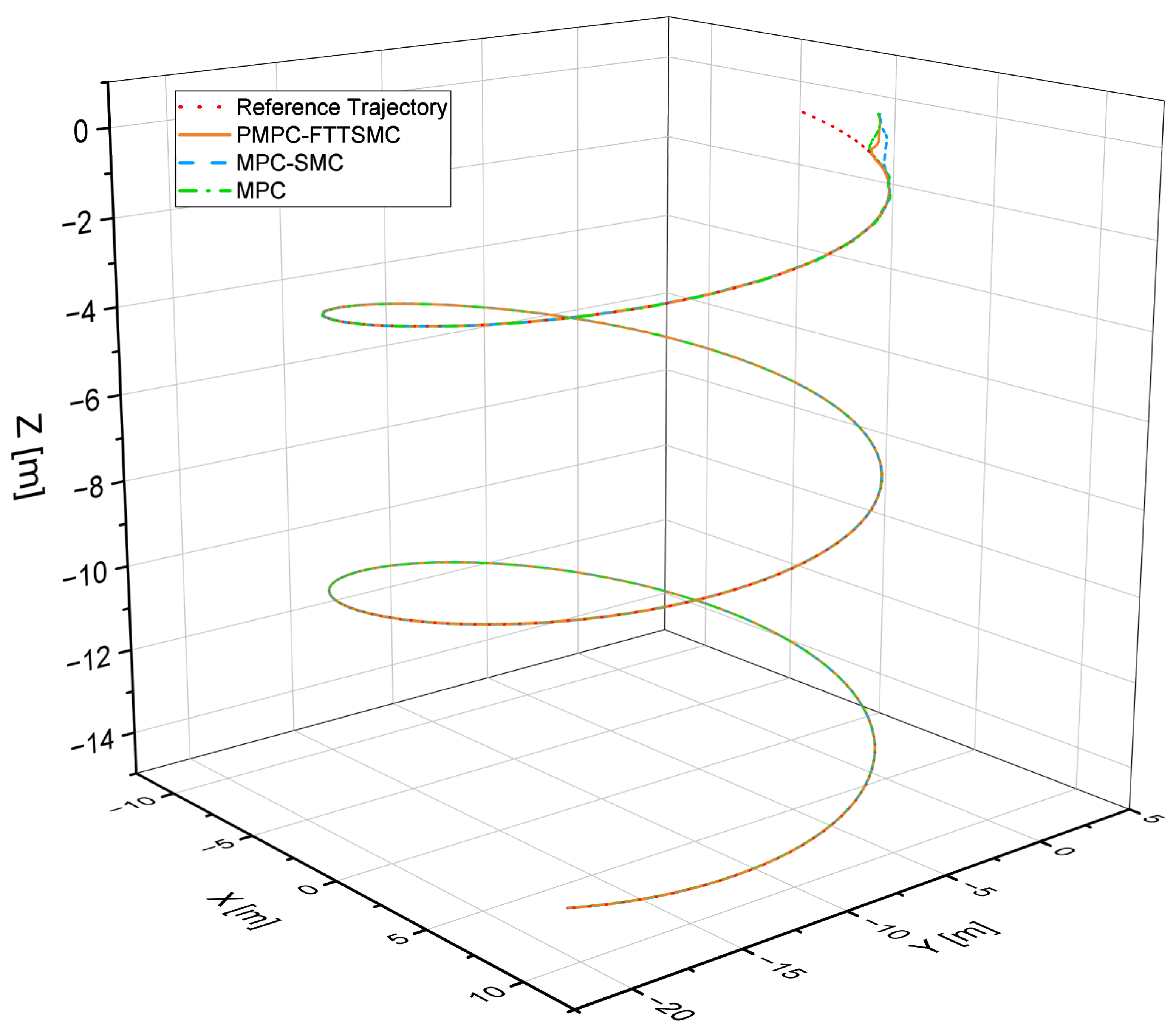
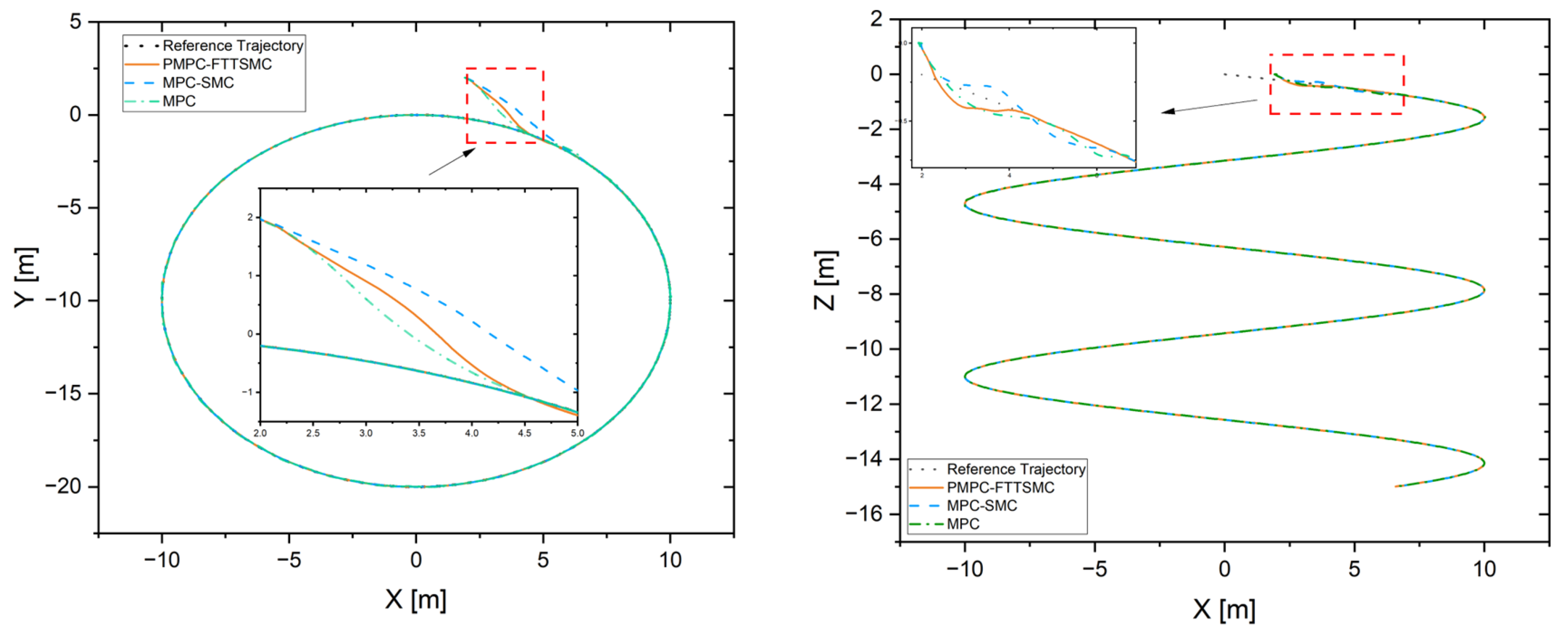
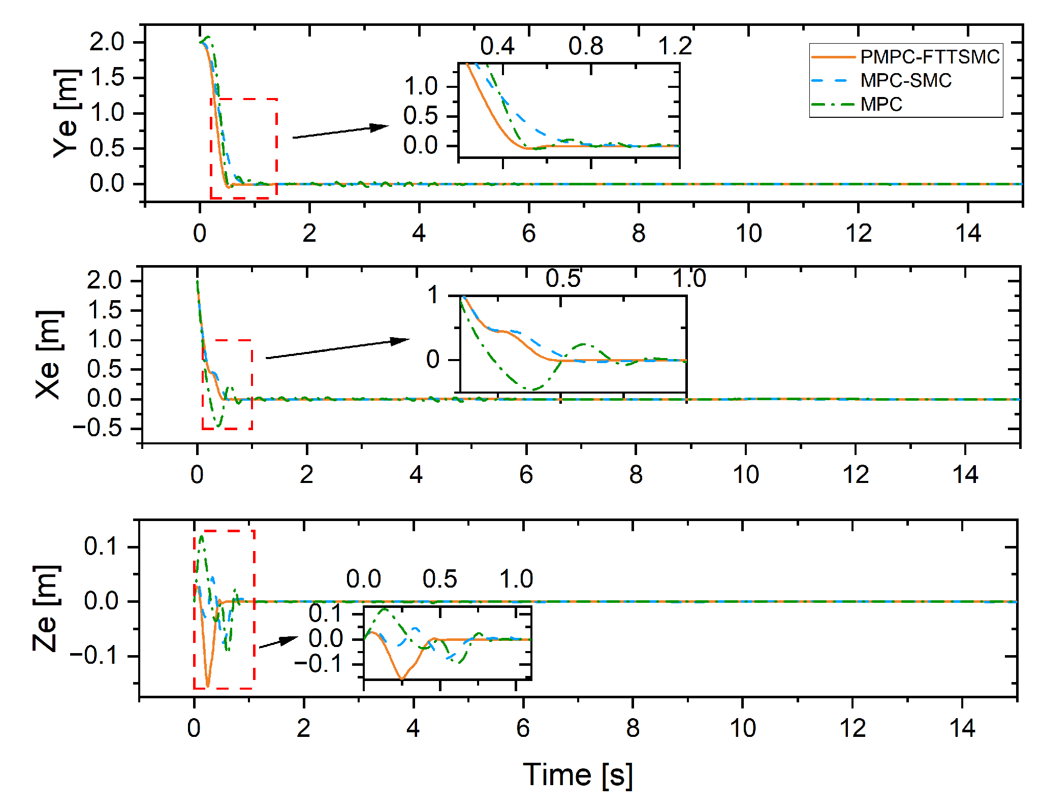
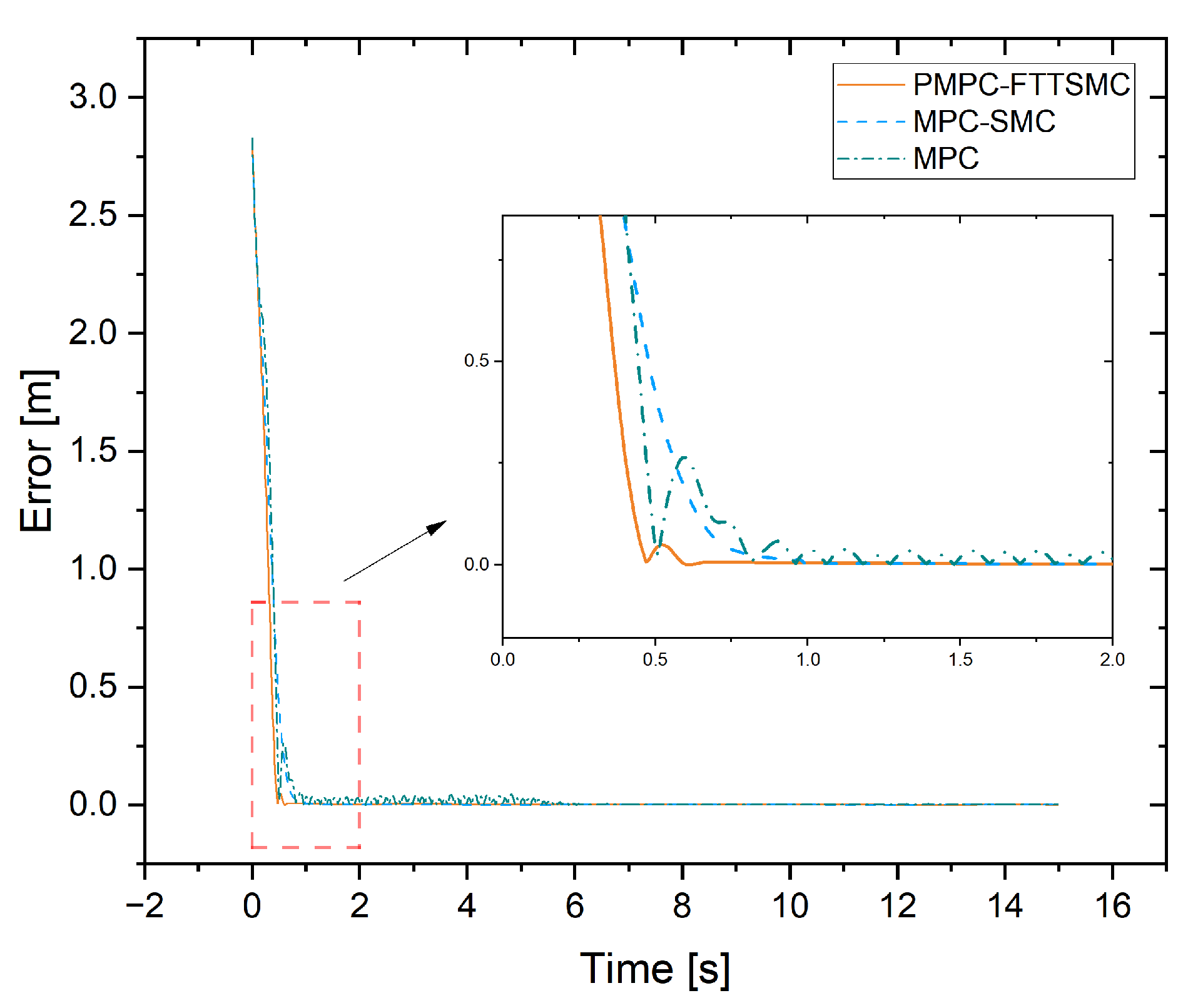
4.2. Case 1: Spiral Trajectory Tracking

In the simulation of case 1, in order to verify the tracking performance of the proposed control method, it was compared with conventional MPC and MPC-SMC methods. UUV is supposed to track an underwater spiral trajectory, which is defined by the following:

$$\left\{\begin{array}{l}{\eta }_{xd}=10\sin (t)\hspace{0.33em}\hspace{0.33em}\hspace{0.33em}\hspace{0.33em}\hspace{0.33em}\hspace{0.33em}\hspace{0.33em}\hspace{0.33em}\hspace{0.33em}\hspace{0.33em}\hspace{0.33em}\hspace{0.33em}m\hfill \\ {\eta }_{yd}=10\cos (t)-10\hspace{0.33em}\hspace{0.33em}\hspace{0.33em}\hspace{0.33em}\hspace{0.33em}\hspace{0.33em}\hspace{0.33em}\hspace{0.33em}m\hfill \\ {\eta }_{zd}=-t\hspace{0.33em}\hspace{0.33em}\hspace{0.33em}\hspace{0.33em}\hspace{0.33em}\hspace{0.33em}\hspace{0.33em}\hspace{0.33em}\hspace{0.33em}\hspace{0.33em}\hspace{0.33em}\hspace{0.33em}\hspace{0.33em}\hspace{0.33em}\hspace{0.33em}\hspace{0.33em}\hspace{0.33em}m\hfill \end{array}\right.$$

(55)

Figure 4 shows underwater spiral trajectory tracking results in 3D space. As shown in the figure, the UUV in all simulations could track the desired trajectory in real time, even in the presence of disturbances. Figure 5 shows the path tracking performance of the three control methods by analyzing their respective XY and XZ axis tracking results. By comparing the path tracking images of the XY and XZ axis for the three methods, the faster speed and better tracking effect of the PMPC-FTTSMC can be clearly shown.

The variation and average number of iterations are presented in Figure 6 and Figure 7, as shown in the figures, and the PMPC-FTTSMC approach achieved an average improvement of 33% and 80% in terms of the number of iterations required in comparison with the MPC-SMC and traditional MPC methods, respectively. PMPC-FTTSMC uses a combination of model predictive control and robust control, which allows for a more efficient optimization process. As a result, the PMPC-FTTSMC algorithm can achieve faster convergence and make real-time decisions more reliably. Tracking errors in the three-axis and overall tracking errors $\sqrt{{\eta }_{xe}^2+{\eta }_{ye}^2+{\eta }_{ze}^2}$ are illustrated in Figure 8 and Figure 9. Based on the simulation results, it was observed that the PMPC-FTTSMC, MPC-SMC, and traditional MPC methods had steady-state times of 0.44 s, 0.68 s, and 0.78 s, respectively. The results suggest that the PMPC-FTTSMC method outperformed the other two approaches, demonstrating an average of 35% reduction in convergence time compared with the MPC-SMC method, and a 44% reduction when compared with the traditional MPC approach. These results suggest that the PMPC-FTTSMC approach may be a more efficient and effective option for certain applications.

In conclusion, PMPC-FTTSMC is a more effective and efficient solution for tracking an underwater spiral trajectory, providing greater stability and accuracy. This conclusion is based on the following factors: PMPC-FTTSMC requires less iteration time to achieve faster convergence compared with the other methods, and it can quickly estimate and reject interference, avoiding constraint violations. The path tracking images in the XY and XZ axes also indicate that the proposed PMPC-FTTSMC can track the desired trajectory more accurately, with less deviation and oscillation. These results suggest that PMPC-FTTSMC can be a better real-time control strategy for UUV path tracking, especially in complex and uncertain underwater environments.

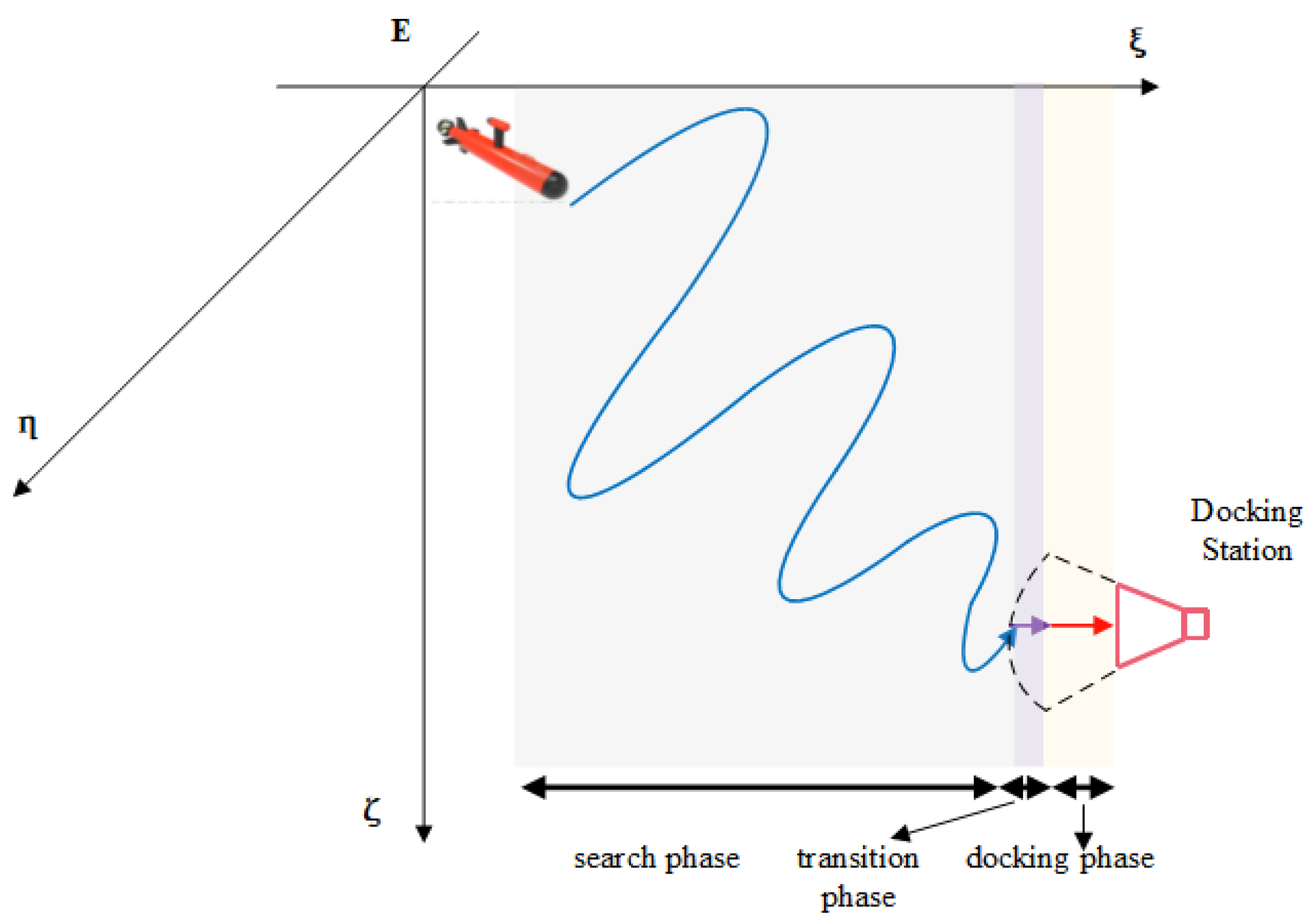
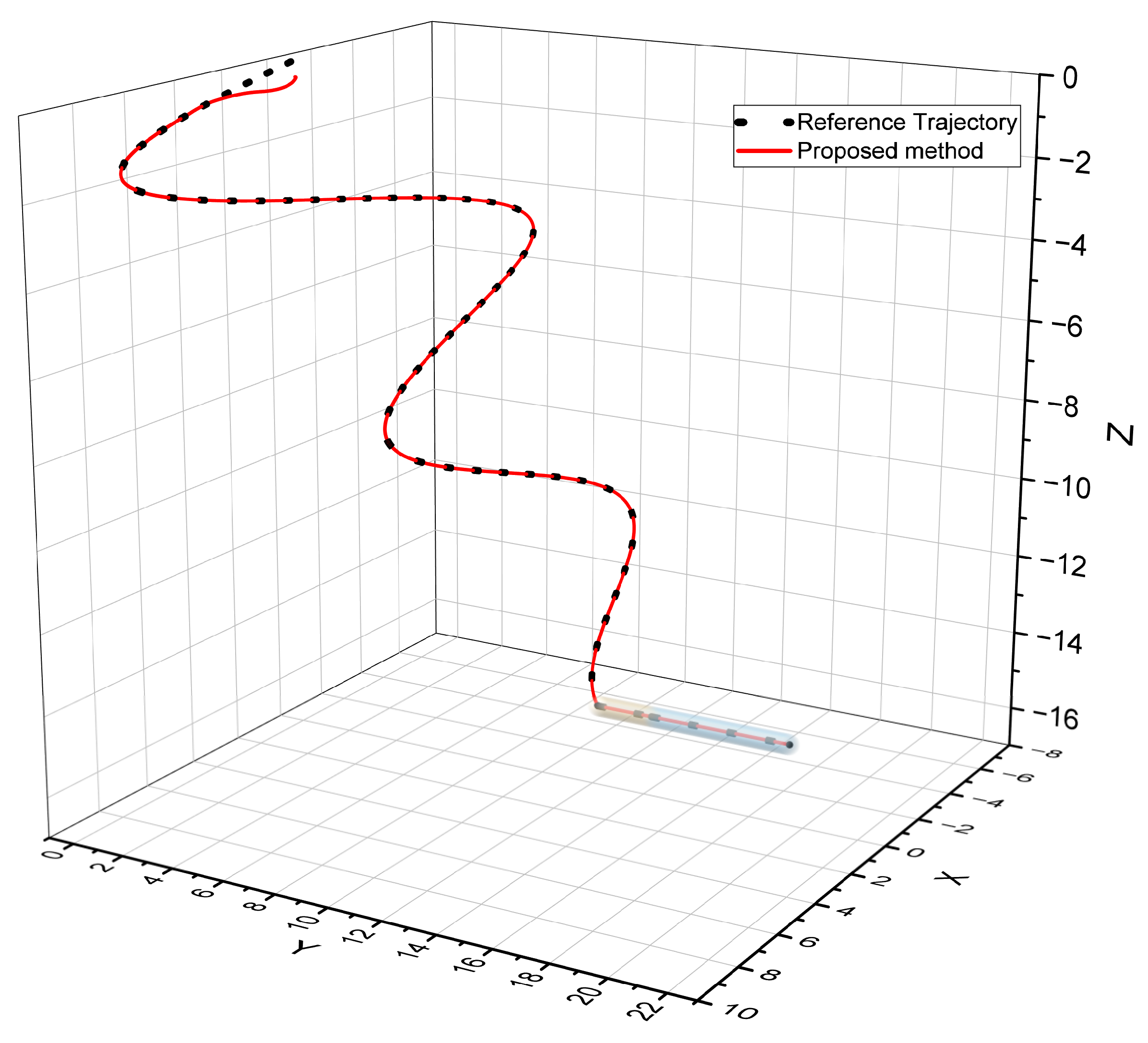
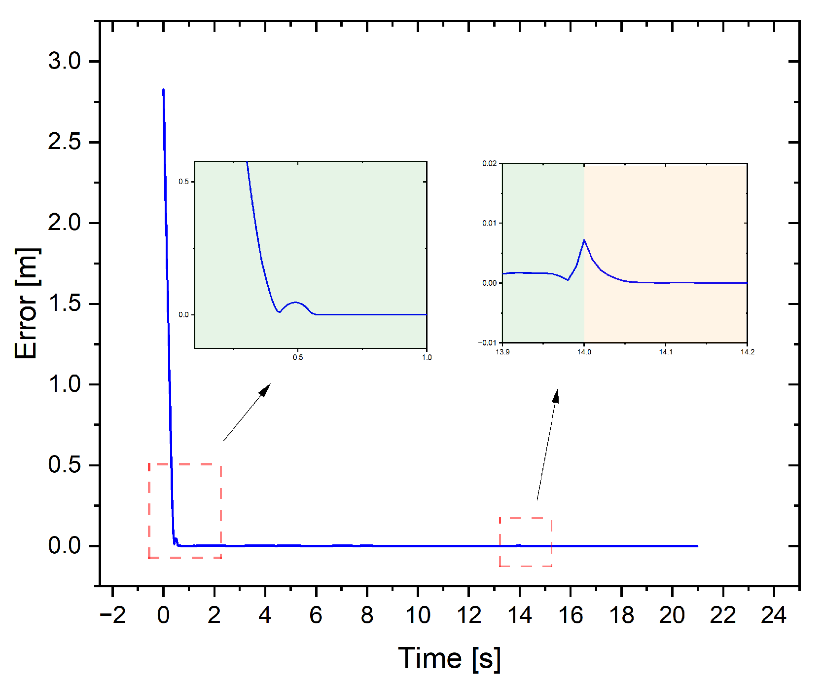
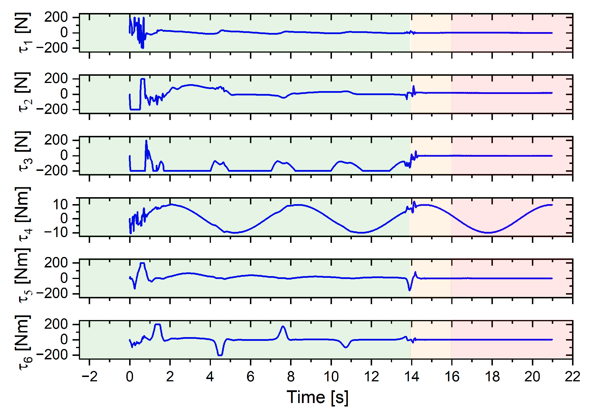
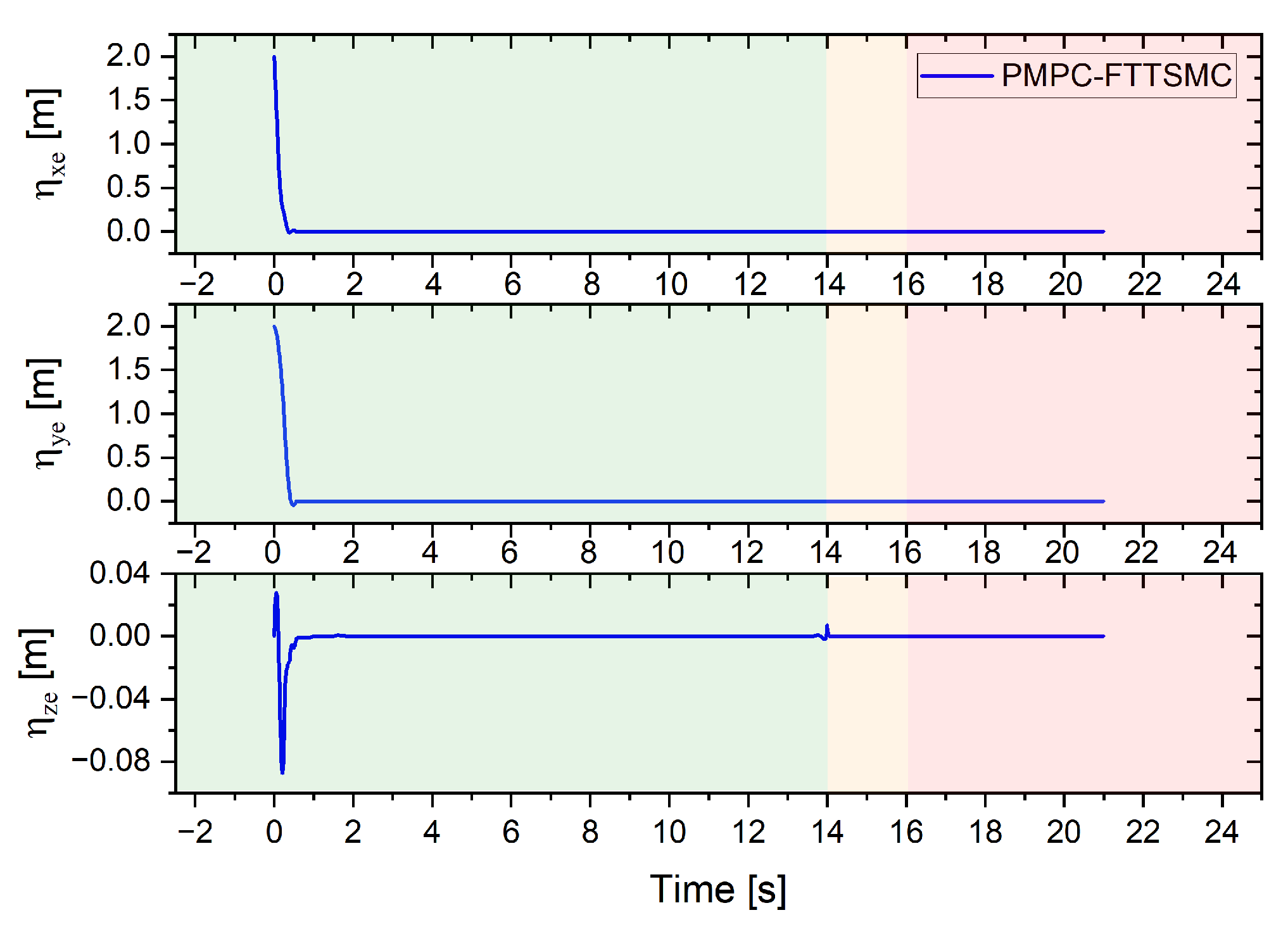
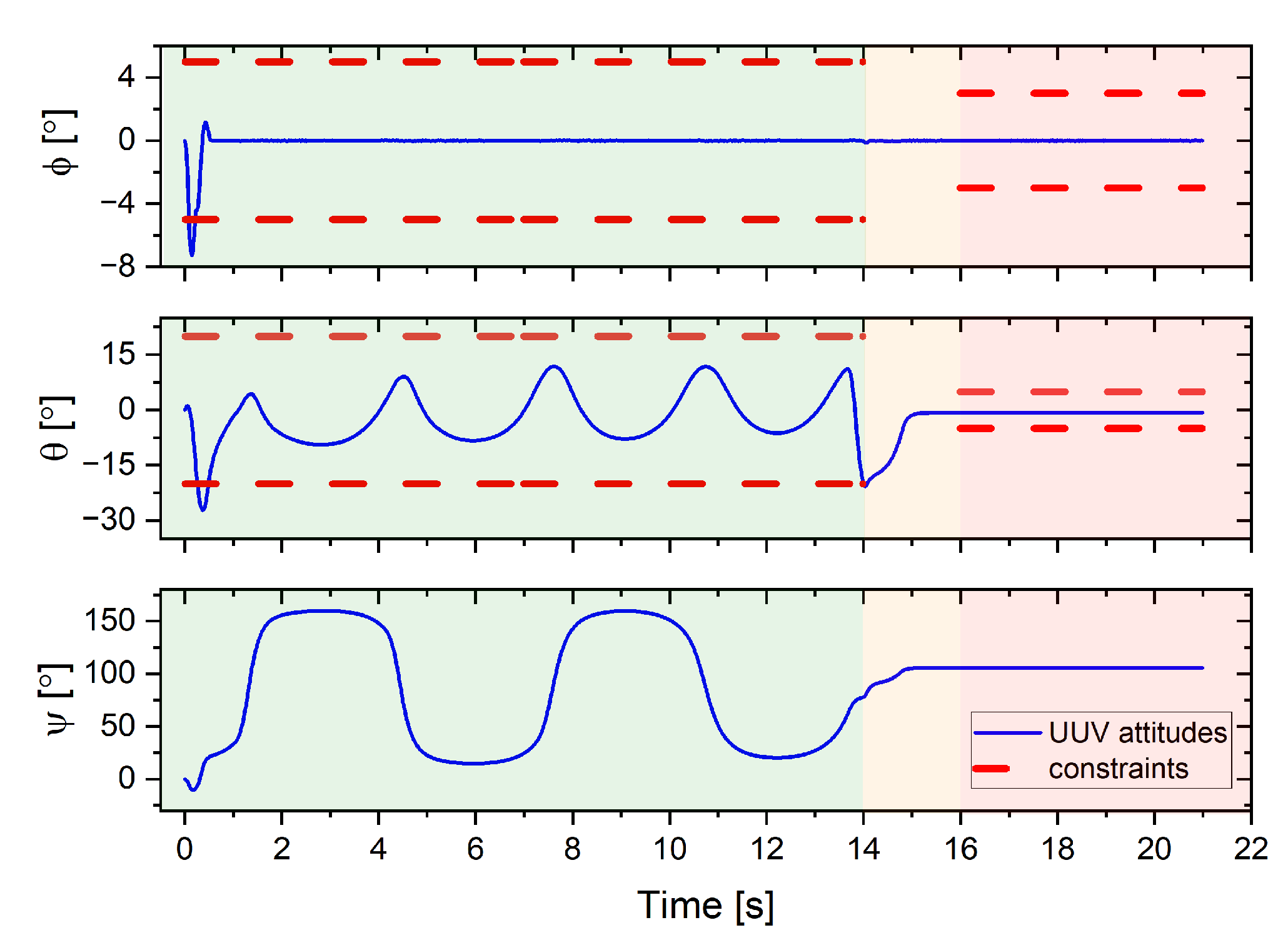
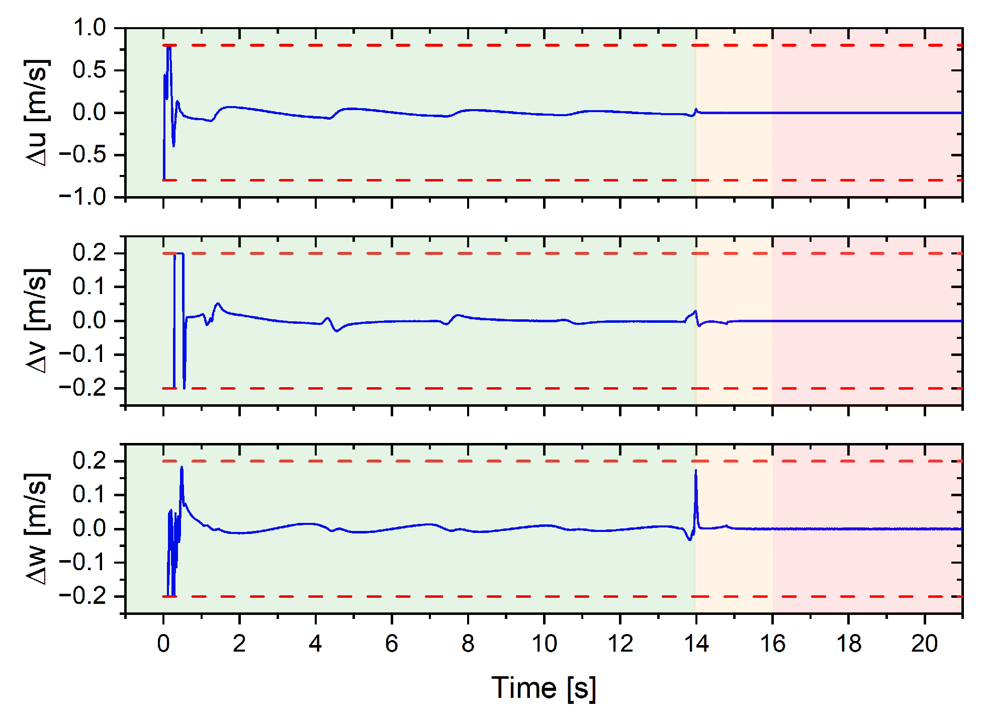
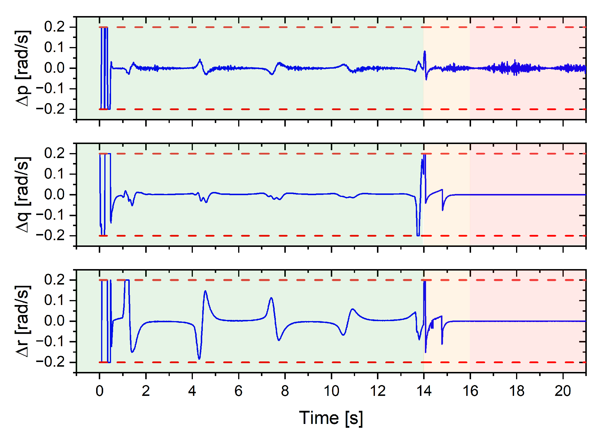
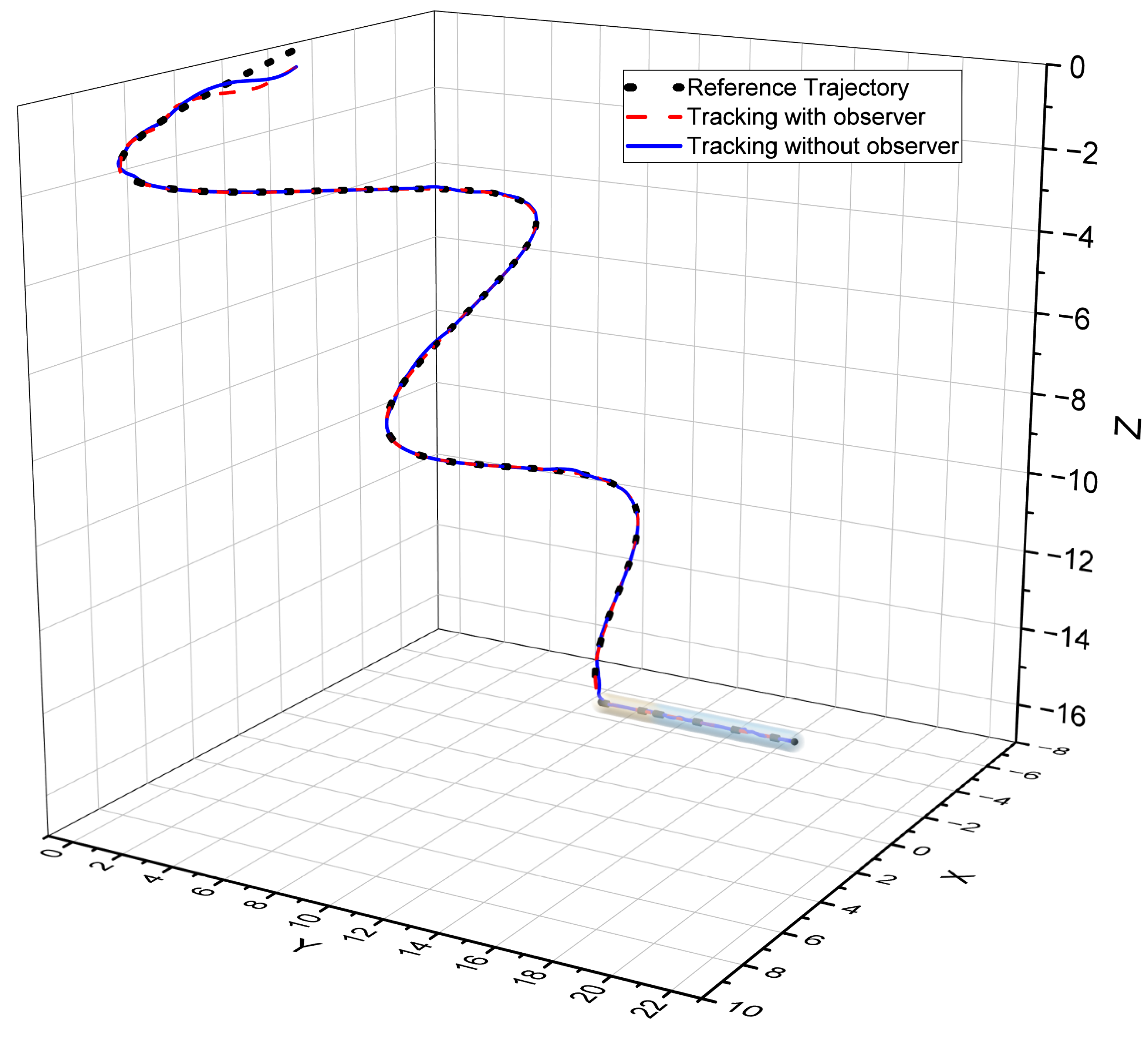
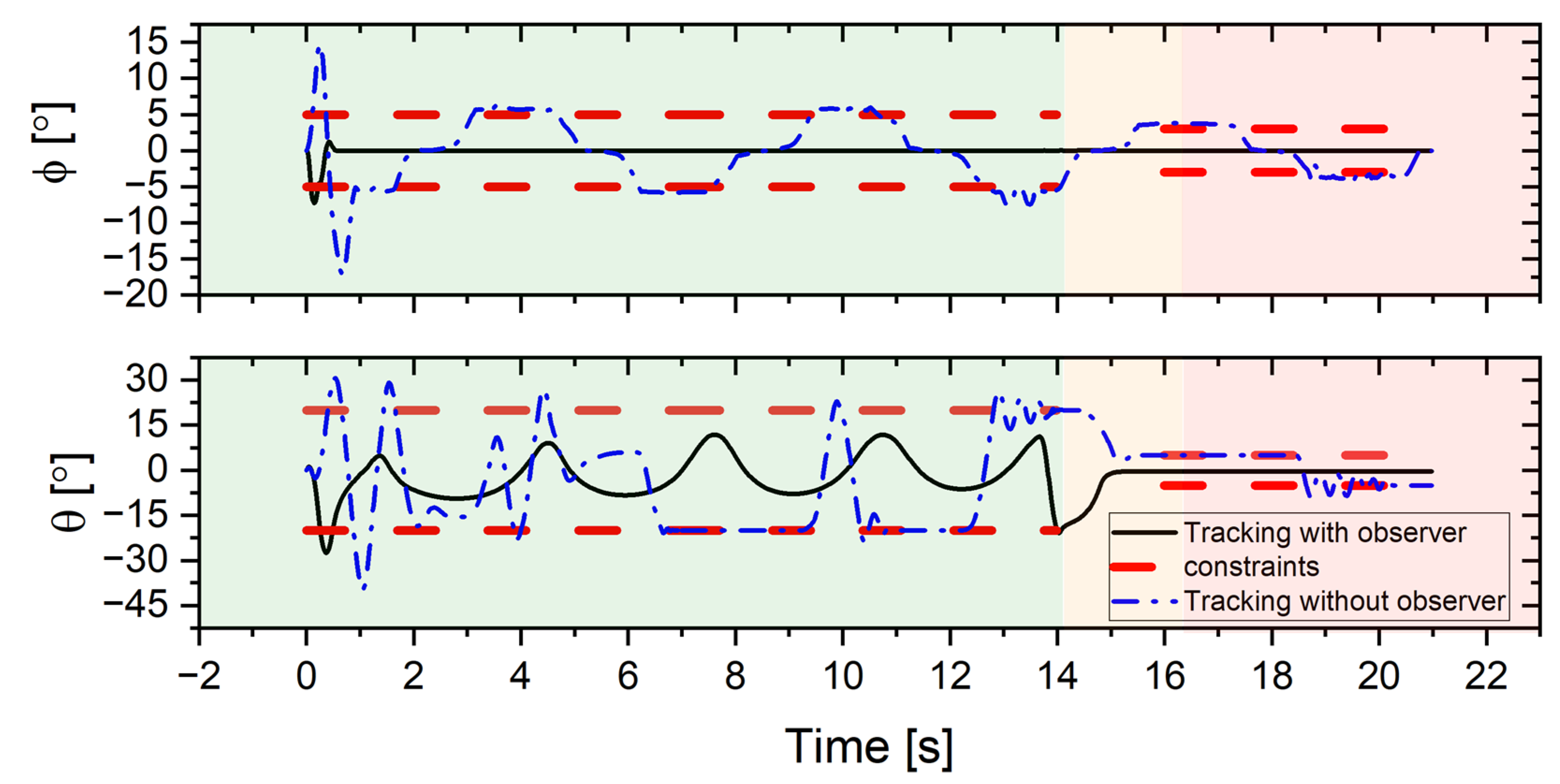
4.3. Case 2: Search-and-Docking Mission

To further prove the superiority of the proposed control algorithm, a search-and-docking mission is presented as an additional test. The objective of the mission is to search along the specified path and dock the UUV with a prescribed performance. This task requires accurate and precise control over the motion and direction of the UUV. It serves as a practical application scenario to assess the effectiveness of the proposed control algorithm for underwater vehicles.

The proposed search-and-docking mission involves the UUV conducting an underwater search following a sinusoidal trajectory and docking along a straight path once it enters the signal range of the docking station. This task is divided into three phases: the search phase, the transition phase, and the docking phase.

During the search phase, the UUV is controlled by the SMPC guidance law. The SMPC allows the UUV to follow the sinusoidal trajectory with minor constraint violations. In the transition phase, both the SMPC and the HMPC are utilized for smooth switching. The HMPC gradually takes over the control from the SMPC within a prescribed time as the UUV approaches the docking station, which ensures that the UUV follows a fast and smooth trajectory tracking during the transition from the search to the docking phase.

In the docking phase, the HMPC is used to strictly control the UUV. The HMPC ensures that the UUV reaches the desired attitude for docking and maintains stability during the docking process. The desired trajectory is designed as follows:

$$p_{d1}=\left\{\begin{array}{l}{\eta }_{xd}=10e^{-0.1t}\cdot \sin (t)\hspace{0.33em}\hspace{0.33em}\hspace{0.33em}\hspace{0.33em}\hspace{0.33em}\hspace{0.33em}\hspace{0.33em}\hspace{0.33em}0<t<14\hfill \\ {\eta }_{yd}=t\hspace{0.33em}\hspace{0.33em}\hspace{0.33em}\hspace{0.33em}\hspace{0.33em}\hspace{0.33em}\hspace{0.33em}\hspace{0.33em}\hspace{0.33em}\hspace{0.33em}\hspace{0.33em}\hspace{0.33em}\hspace{0.33em}\hspace{0.33em}\hspace{0.33em}\hspace{0.33em}\hspace{0.33em}\hspace{0.33em}0<t<14\hfill \\ {\eta }_{zd}=-t\hspace{0.33em}\hspace{0.33em}\hspace{0.33em}\hspace{0.33em}\hspace{0.33em}\hspace{0.33em}\hspace{0.33em}\hspace{0.33em}\hspace{0.33em}\hspace{0.33em}\hspace{0.33em}\hspace{0.33em}\hspace{0.33em}\hspace{0.33em}\hspace{0.33em}\hspace{0.33em}\hspace{0.33em}\hspace{0.33em}0<t<14\hfill \end{array}\right.$$

(56)

$$p_{d2}=\left\{\begin{array}{l}{\eta }_{xd}=14\hspace{0.33em}\hspace{0.33em}\hspace{0.33em}\hspace{0.33em}\hspace{0.33em}\hspace{0.33em}\hspace{0.33em}\hspace{0.33em}\hspace{0.33em}\hspace{0.33em}\hspace{0.33em}\hspace{0.33em}\hspace{0.33em}\hspace{0.33em}\hspace{0.33em}\hspace{0.33em}\hspace{0.33em}\hspace{0.33em}\hspace{0.33em}\hspace{0.33em}14<t<21\hfill \\ {\eta }_{yd}=t\hspace{0.33em}\hspace{0.33em}\hspace{0.33em}\hspace{0.33em}\hspace{0.33em}\hspace{0.33em}\hspace{0.33em}\hspace{0.33em}\hspace{0.33em}\hspace{0.33em}\hspace{0.33em}\hspace{0.33em}\hspace{0.33em}\hspace{0.33em}\hspace{0.33em}\hspace{0.33em}\hspace{0.33em}\hspace{0.33em}\hspace{0.33em}\hspace{0.33em}14<t<21\hfill \\ {\eta }_{zd}=-14\hspace{0.33em}\hspace{0.33em}\hspace{0.33em}\hspace{0.33em}\hspace{0.33em}\hspace{0.33em}\hspace{0.33em}\hspace{0.33em}\hspace{0.33em}\hspace{0.33em}\hspace{0.33em}\hspace{0.33em}\hspace{0.33em}\hspace{0.33em}\hspace{0.33em}\hspace{0.33em}\hspace{0.33em}\hspace{0.33em}\hspace{0.33em}14<t<21\hfill \end{array}\right.$$

(57)

Figure 10 shows the trajectory tracking results of the mission in 3D space. The black dots are the desired trajectory, the red curve is the simulated tracking result of the proposed, the yellow pipe part is the transition phase, and the blue pipe part is the docking phase. It is easily seen that the proposed control method can achieve good trajectory tracking. To better analyze the tracking performances of different stages, three different background colors are used to mark each stage in Figure 11, Figure 12, Figure 13, Figure 14, Figure 15, Figure 16, Figure 17 and Figure 18. The green background represents the search phase, the orange background represents the transition phase, and the red background represents the docking phase. The output of the dynamic controller is shown in Figure 12. The transitions of overall tracking errors and tracking errors in the three-axis are illustrated in Figure 11 and Figure 13, which clearly show that there are relatively small overshoots and reduced chattering for the proposed method. This is because the proposed method incorporates an integral term into the sliding surface design. It smooths out the control action and reduces the abrupt switching behavior typically associated with chattering. As a result, the proposed method effectively enhances the system’s response and ensures a better overall performance. The attitude of the UUV is demonstrated in Figure 14, where it can be seen that the attitude variables of the UUV can break through constraints during the search phase, while UUV strictly obeys the constraints during the docking phase. The velocity and angular velocity increment are shown in Figure 15 and Figure 16, and it can be seen that the UUV always satisfies the hard constraint of velocity smoothness in the whole stage of the trajectory tracking. The variation of iterations is presented in Figure 17. As shown in Figure 18, the weight allocator provides smooth weights for controller switching. The disturbance estimation results of six degrees of freedom and a comparison between FTRBFNN and asymptotically convergent RBFNN are given in Figure 19 and Figure 20. It is obvious that the proposed method has a significant advantage in terms of interference estimation. PMPC-FTTSMC utilizes FTRBFDO, which allows for a fast and accurate estimate of the interference signal. This improves the overall accuracy of the tracking results and helps to mitigate the impact of disturbances in the system. To further validate the robustness of the proposed algorithm, Figure 21, Figure 22 and Figure 23 demonstrate the trajectory tracking performance of the UUV and the disturbance estimation results when the disturbance amplitude is doubled. As shown in the figures, the proposed algorithm is capable of maintaining effective trajectory tracking and accurate disturbance estimation, even in the presence of larger disturbances. During precise docking, accurate control of the UUV’s attitude is crucial for successful operation. From Figure 22, it can be observed that the disturbance observer significantly improves the control performance of roll and pitch angles even in the presence of large disturbances. This enhancement ensures that the UUV maintains the desired performance during precise docking processes.

Based on the analyses above, it is easy to draw the following conclusions. The proposed control algorithm can provide fast and accurate trajectory tracking, while ensuring stability and robustness in the presence of disturbances. The success of the search-and-docking mission further validates the effectiveness and efficiency of the proposed PMPC-FTTSMC algorithm in real-world scenarios for UUV docking.

4.4. Discussion of Results

In case 1, a comparison of three control methods (traditional MPC, MPC-SMC, and PMPC-FTTSMC) is presented for underwater spiral trajectory tracking. The simulation results demonstrate that the proposed PMPC-FTTSMC control method outperforms the other two approaches in terms of faster convergence, higher accuracy, and greater stability, even in the presence of disturbances. The PMPC-FTTSMC approach achieved an average improvement of 33% and 80% in terms of the number of iterations required in comparison to the MPC-SMC and traditional MPC methods, respectively. The path tracking images of the XY and XZ axes also indicate that the proposed PMPC-FTTSMC can track the desired trajectory more accurately, with less deviation and oscillation. Based on the simulation results, it can be concluded that PMPC-FTTSMC is a more efficient and effective option for certain underwater applications.

In case 2, the trajectory tracking results for a search-and-docking mission using the proposed PMPC-FTTSMC control algorithm are presented. The analysis of tracking performances of different stages indicates that the proposed method achieves relatively small overshoots and reduced chattering. The attitude, velocity, and angular velocity increment of the UUV are strictly controlled during the docking phase, and the proposed algorithm is capable of accurate disturbance estimation, even in the presence of larger disturbances.

In summary, the algorithm proposed in this paper has the ability to effectively handle diverse constraints in complex multi-stage scenarios. It demonstrates rapid and stable error convergence, while also significantly reducing iteration time and hardware requirements. As a result, it holds vast potential for applications in various fields.

5. Conclusions

In this paper, a novel control algorithm based on PMPC-FTTSMC is proposed to achieve the prescribed performance trajectory tracking control of a UUV. Firstly, the 6-DOF kinematics and dynamics model of a fully-actuated UUV are presented. Secondly, the input, state constraints, and velocity finite time convergence are considered as the prescribed performance in the PMPC guidance law and dynamic control law. Finally, a comparative simulation of two different scenarios is carried out: In the first case, the proposed controller is compared with traditional MPC and MPC-SMC methods in terms of tracking performance and computational efficiency. The simulation results demonstrate that the PMPC-FTTSMC approach outperformed the MPC-SMC and traditional MPC methods in terms of the number of iterations required, achieving an average improvement of 33% and 80%, respectively. Furthermore, the PMPC-FTTSMC method exhibited a significant reduction in convergence time, with an average of 35% and 44% improvement compared with the MPC-SMC and traditional MPC approaches, respectively. In the second case, a search-and-docking mission was also designed to further verify the effectiveness and feasibility of the proposed algorithm in practical applications. It is shown that the PMPC-FTTSMC could achieve fast interference estimation and convergence, as well as improve the tracking accuracy and stability of the UUV. The use of PMPC-FTTSMC in prescribed performance control allows for a robust, constraint-aware control scheme that can achieve the desired performance specifications within a finite time horizon. The combination of parallel controller, fast interference estimation, and robust constraint handling makes the proposed method a promising approach for real-time control and decision-making in complex underwater systems.

However, it is important to note that the proposed method does have some limitations. The presented UUV model makes several idealized assumptions to simplify the calculations and analysis. Uncertainties in the UUV’s hydrodynamics and environmental factors are treated as combined disturbances and estimated by a disturbance observer, without specifically analyzing the impact of individual factors that contribute to the composite disturbance. The impact of these individual factors on the performance of the control system is an important aspect that will be investigated in future work. In addition, future work could also explore the combination of the proposed PMPC-FTTSMC algorithm with fault-tolerant control algorithms. This would allow for greater robustness to unexpected events or faults in the UUV’s hardware or software, increasing the safety and reliability of the system in real-world applications.

References

1. Bruzzone, G.; Ferretti, R.; Odetti, A. Unmanned Marine Vehicles. J. Mar. Sci. Eng. 2021, 9, 257. [Google Scholar] [CrossRef]
2. Stateczny, A.; Gronska-Sledz, D.; Motyl, W. Precise Bathymetry as a Step Towards Producing Bathymetric Electronic Navigational Charts for Comparative (Terrain Reference) Navigation. J. Navig. 2019, 72, 1623–1632. [Google Scholar] [CrossRef]
3. Marini, S.; Gjeci, N.; Govindaraj, S.; But, A.; Sportich, B.; Ottaviani, E.; Márquez, F.P.G.; Bernalte Sanchez, P.J.; Pedersen, J.; Clausen, C.V. Enduruns: An Integrated and Flexible Approach for Seabed Survey through Autonomous Mobile Vehicles. J. Mar. Sci. Eng. 2020, 8, 633. [Google Scholar] [CrossRef]
4. Kim, J. Cooperative Localisation for Deep-Sea Exploration Using Multiple Unmanned Underwater Vehicles. IET Radar Sonar Navig. 2020, 14, 1244–1248. [Google Scholar] [CrossRef]
5. Ryu, J.H. Prototyping a Low-Cost Open-Source Autonomous Unmanned Surface Vehicle for Real-Time Water Quality Monitoring and Visualization. Hardwarex 2022, 12, e369. [Google Scholar] [CrossRef]
6. González-García, J.; Gómez-Espinosa, A.; García-Valdovinos, L.G.; Salgado-Jiménez, T.; Cuan-Urquizo, E.; Escobedo Cabello, J.A. Experimental Validation of a Model-Free High-Order Sliding Mode Controller with Finite-Time Convergence for Trajectory Tracking of Autonomous Underwater Vehicles. Sensors 2022, 22, 488. [Google Scholar] [CrossRef] [PubMed]
7. Manzanilla, A.; Ibarra, E.; Salazar, S.; Zamora, Á.E.; Lozano, R.; Munoz, F. Super-Twisting Integral Sliding Mode Control for Trajectory Tracking of an Unmanned Underwater Vehicle. Ocean. Eng. 2021, 234, 109164. [Google Scholar] [CrossRef]
8. Kim, J.H.; Yoo, S.J. Distributed Event-Triggered Adaptive Output-Feedback Formation Tracking of Uncertain Underactuated Underwater Vehicles in Three-Dimensional Space. Appl. Math. Comput. 2022, 424, 127046. [Google Scholar] [CrossRef]
9. Li, D.; Du, L. Auv Trajectory Tracking Models and Control Strategies: A Review. J. Mar. Sci. Eng. 2021, 9, 1020. [Google Scholar] [CrossRef]
10. Gutnik, Y.; Avni, A.; Treibitz, T.; Groper, M. On the Adaptation of an Auv Into a Dedicated Platform for Close Range Imaging Survey Missions. J. Mar. Sci. Eng. 2022, 10, 974. [Google Scholar] [CrossRef]
11. Cervantes, J.; Yu, W.; Salazar, S.; Chairez, I.; Lozano, R. Output Based Backstepping Control for Trajectory Tracking of an Autonomous Underwater Vehicle. In Proceedings of the 2016 American Control Conference (ACC), Boston, MA, USA, 6–8 July 2016. [Google Scholar]
12. Liang, X.; Wan, L.; Blake, J.I.; Shenoi, R.A.; Townsend, N. Path Following of an Underactuated Auv Based On Fuzzy Backstepping Sliding Mode Control. Int. J. Adv. Robot. Syst. 2016, 13, 122. [Google Scholar] [CrossRef] [Green Version]
13. Yu, C.; Xiang, X.; Wilson, P.A.; Zhang, Q. Guidance-Error-Based Robust Fuzzy Adaptive Control for Bottom Following of a Flight-Style Auv with Saturated Actuator Dynamics. IEEE Trans. Cybern. 2019, 50, 1887–1899. [Google Scholar] [CrossRef] [Green Version]
14. Li, X.; Liu, Y. A New Fuzzy Smc Control Approach to Path Tracking of Autonomous Underwater Vehicles with Mismatched Disturbances. In Proceedings of the OCEANS 2022-Chennai, Chennai, India, 21–24 February 2022. [Google Scholar]
15. Rodriguez, J.; Castañeda, H.; Gordillo, J.L. Design of an Adaptive Sliding Mode Control for a Micro-Auv Subject to Water Currents and Parametric Uncertainties. J. Mar. Sci. Eng. 2019, 7, 445. [Google Scholar] [CrossRef] [Green Version]
16. Londhe, P.S.; Patre, B.M. Adaptive Fuzzy Sliding Mode Control for Robust Trajectory Tracking Control of an Autonomous Underwater Vehicle. Intell. Serv. Robot. 2019, 12, 87–102. [Google Scholar] [CrossRef]
17. Chu, Z.; Xiang, X.; Zhu, D.; Luo, C.; Xie, D. Adaptive Trajectory Tracking Control for Remotely Operated Vehicles Considering Thruster Dynamics and Saturation Constraints. Isa Trans. 2020, 100, 28–37. [Google Scholar] [CrossRef]
18. Barreno, P.; Parras, J.; Zazo, S. An Efficient Underwater Navigation Method Using Mpc with Unknown Kinematics and Non-Linear Disturbances. J. Mar. Sci. Eng. 2023, 11, 710. [Google Scholar] [CrossRef]
19. Lakhekar, G.V.; Waghmare, L.M.; Roy, R.G. Disturbance Observer-Based Fuzzy Adapted S-Surface Controller for Spatial Trajectory Tracking of Autonomous Underwater Vehicle. IEEE Trans. Intell. Veh. 2019, 4, 622–636. [Google Scholar] [CrossRef]
20. Xia, Y.; Xu, K.; Wang, W.; Xu, G.; Xiang, X.; Li, Y. Optimal Robust Trajectory Tracking Control of a X-Rudder Auv with Velocity Sensor Failures and Uncertainties. Ocean. Eng. 2020, 198, 106949. [Google Scholar] [CrossRef]
21. Gan, W.; Zhu, D.; Ji, D. Qpso-Model Predictive Control-Based Approach to Dynamic Trajectory Tracking Control for Unmanned Underwater Vehicles. Ocean. Eng. 2018, 158, 208–220. [Google Scholar] [CrossRef]
22. Ahmad, S.; Uppal, A.A.; Azam, M.R.; Iqbal, J. Chattering Free Sliding Mode Control and State Dependent Kalman Filter Design for Underground Gasification Energy Conversion Process. Electronics 2023, 12, 876. [Google Scholar] [CrossRef]
23. Yu, H.; Guo, C.; Yan, Z. Globally Finite-Time Stable Three-Dimensional Trajectory-Tracking Control of Underactuated Uuvs. Ocean. Eng. 2019, 189, 106329. [Google Scholar] [CrossRef]
24. Pan, J.; Liu, J.; Yu, J. Path-Following Control of an Amphibious Robotic Fish Using Fuzzy-Linear Model Predictive Control Approach. In Proceedings of the 2020 IEEE International Conference on Mechatronics and Automation (ICMA), Beijing, China, 13–16 October 2020. [Google Scholar]
25. Khodayari, M.H.; Balochian, S. Modeling and Control of Autonomous Underwater Vehicle (Auv) in Heading and Depth Attitude Via Self-Adaptive Fuzzy Pid Controller. J. Mar. Sci. Technol. 2015, 20, 559–578. [Google Scholar] [CrossRef]
26. Sun, B.; Gan, W.; Zhu, D.; Zhang, W.; Yang, S.X. A Model Predictive Based Uuv Control Design From Kinematic to Dynamic Tracking Control. In Proceedings of the 2017 36th Chinese Control Conference (CCC), Dalian, China, 26–28 July 2017. [Google Scholar]
27. von Ellenrieder, K.D. Dynamic Surface Control of Trajectory Tracking Marine Vehicles with Actuator Magnitude and Rate Limits. Automatica 2019, 105, 433–442. [Google Scholar] [CrossRef]
28. Cui, R.; Chen, L.; Yang, C.; Chen, M. Extended State Observer-Based Integral Sliding Mode Control for an Underwater Robot with Unknown Disturbances and Uncertain Nonlinearities. IEEE Trans. Ind. Electron. 2017, 64, 6785–6795. [Google Scholar] [CrossRef] [Green Version]
29. Rojsiraphisal, T.; Mobayen, S.; Asad, J.H.; Vu, M.T.; Chang, A.; Puangmalai, J. Fast Terminal Sliding Control of Underactuated Robotic Systems Based On Disturbance Observer with Experimental Validation. Mathematics 2021, 9, 1935. [Google Scholar] [CrossRef]
30. He, S.; Dai, S.; Zhao, Z.; Zou, T. Uncertainty and Disturbance Estimator-Based Distributed Synchronization Control for Multiple Marine Surface Vehicles with Prescribed Performance. Ocean. Eng. 2022, 261, 111867. [Google Scholar] [CrossRef]
31. Shen, Z.; Wang, Q.; Dong, S.; Yu, H. Prescribed Performance Dynamic Surface Control for Trajectory-Tracking of Unmanned Surface Vessel with Input Saturation. Appl. Ocean. Res. 2021, 113, 102736. [Google Scholar] [CrossRef]
32. Kim, J.H.; Yoo, S.J. Adaptive Event-Triggered Control Strategy for Ensuring Predefined Three-Dimensional Tracking Performance of Uncertain Nonlinear Underactuated Underwater Vehicles. Mathematics 2021, 9, 137. [Google Scholar] [CrossRef]
33. Liang, H.; Fu, Y.; Gao, J.; Cao, H. Finite-Time Velocity-Observed Based Adaptive Output-Feedback Trajectory Tracking Formation Control for Underactuated Unmanned Underwater Vehicles with Prescribed Transient Performance. Ocean. Eng. 2021, 233, 109071. [Google Scholar] [CrossRef]
34. Ding, Z.; Wang, H.; Sun, Y.; Qin, H. Adaptive Prescribed Performance Second-Order Sliding Mode Tracking Control of Autonomous Underwater Vehicle Using Neural Network-Based Disturbance Observer. Ocean. Eng. 2022, 260, 111939. [Google Scholar] [CrossRef]
35. Dai, S.; Wang, M.; Wang, C. Neural Learning Control of Marine Surface Vessels with Guaranteed Transient Tracking Performance. IEEE Trans. Ind. Electron. 2015, 63, 1717–1727. [Google Scholar] [CrossRef]
36. Ahmed, A.; Javed, S.B.; Uppal, A.A.; Iqbal, J. Development of Cavlab—A Control-Oriented Matlab Based Simulator for an Underground Coal Gasification Process. Mathematics 2023, 11, 2493. [Google Scholar] [CrossRef]
37. Zhang, Y.; Liu, X.; Luo, M.; Yang, C. Mpc-Based 3-D Trajectory Tracking for an Autonomous Underwater Vehicle with Constraints in Complex Ocean Environments. Ocean. Eng. 2019, 189, 106309. [Google Scholar] [CrossRef]
38. Gong, P.; Yan, Z.; Zhang, W.; Tang, J. Trajectory Tracking Control for Autonomous Underwater Vehicles Based On Dual Closed-Loop of Mpc with Uncertain Dynamics. Ocean. Eng. 2022, 265, 112697. [Google Scholar] [CrossRef]
39. Zhang, W.; Wang, Q.; Wu, W.; Du, X.; Zhang, Y.; Han, P. Event-Trigger Nmpc for 3-D Trajectory Tracking of Uuv with External Disturbances. Ocean. Eng. 2023, 283, 115050. [Google Scholar] [CrossRef]
40. Gomes, R.; Pereira, F.L. A General Attainable-Set Model Predictive Control Scheme. Application to Auv Operations. Ifac-Papersonline 2018, 51, 314–319. [Google Scholar] [CrossRef]
41. Shen, C.; Shi, Y. Distributed Implementation of Nonlinear Model Predictive Control for Auv Trajectory Tracking. Automatica 2020, 115, 108863. [Google Scholar] [CrossRef]
42. Richards, A. Fast Model Predictive Control with Soft Constraints. Eur. J. Control 2015, 25, 51–59. [Google Scholar] [CrossRef]
43. Oliveira, É.L.; Orsino, R.M.; Donha, D.C. Disturbance-Observer-Based Model Predictive Control of Underwater Vehicle Manipulator Systems. Ifac-Papersonline 2021, 54, 348–355. [Google Scholar] [CrossRef]
44. Fossen, T.I. Handbook of Marine Craft Hydrodynamics and Motion Control; John Wiley & Sons: Hoboken, NJ, USA, 2011. [Google Scholar]
45. Yu, S.; Yu, X.; Shirinzadeh, B.; Man, Z. Continuous Finite-Time Control for Robotic Manipulators with Terminal Sliding Mode. Automatica 2005, 41, 1957–1964. [Google Scholar] [CrossRef]
46. Wang, R.; Tang, L.; Yang, Y.; Wang, S.; Tan, M.; Xu, C. Adaptive Trajectory Tracking Control with Novel Heading Angle and Velocity Compensation for Autonomous Underwater Vehicles. Ieee Transactions On Intelligent Vehicles. IEEE Trans. Intell. Veh. 2023, 8, 2135–2147. [Google Scholar] [CrossRef]
47. Wang, H.; Su, B. Event-Triggered Formation Control of Auvs with Fixed-Time Rbf Disturbance Observer. Appl. Ocean. Res. 2021, 112, 102638. [Google Scholar] [CrossRef]
48. Xia, Y.; Xu, K.; Huang, Z.; Wang, W.; Xu, G.; Li, Y. Adaptive Energy-Efficient Tracking Control of a X Rudder Auv with Actuator Dynamics and Rolling Restriction. Appl. Ocean. Res. 2022, 118, 102994. [Google Scholar] [CrossRef]
49. Qiao, L.; Zhang, W. Double-Loop Integral Terminal Sliding Mode Tracking Control for Uuvs with Adaptive Dynamic Compensation of Uncertainties and Disturbances. IEEE J. Ocean. Eng. 2018, 44, 29–53. [Google Scholar] [CrossRef]
50. Xia, Y.; Huang, Z.; Xu, K.; Xu, G.; Li, Y. Three-Dimensional Trajectory Tracking for a Heterogeneous Xauv Via Finite-Time Robust Nonlinear Control and Optimal Rudder Allocation. J. Mar. Sci. Eng. 2022, 10, 1297. [Google Scholar] [CrossRef]
51. Yan, Z.; Gong, P.; Zhang, W.; Wu, W. Model Predictive Control of Autonomous Underwater Vehicles for Trajectory Tracking with External Disturbances. Ocean. Eng. 2020, 217, 107884. [Google Scholar] [CrossRef]
52. Prestero, T.T.J. Verification of a Six-Degree of Freedom Simulation Model for the Remus Autonomous Underwater Vehicle; Massachusetts Institute of Technology: Cambridge, MA, USA, 2001. [Google Scholar]
53. Andersson, J.A.; Gillis, J.; Horn, G.; Rawlings, J.B.; Diehl, M. CasADi: A Software Framework for Nonlinear Optimization and Optimal Control. Math. Program. Comput. 2019, 11, 1–36. [Google Scholar] [CrossRef]
Figure 1. Coordinate system.
Jmse 11 01357 g001
Figure 2. UUV search-and-docking mission.
Jmse 11 01357 g002
Figure 3. The proposed trajectory tracking control scheme.
Jmse 11 01357 g003
Figure 4. The 3D trajectory tracking comparison of Case 1.
Jmse 11 01357 g004
Figure 5. The 2D profile comparison of Case 1.
Jmse 11 01357 g005
Figure 6. The number of iterations over time.
Jmse 11 01357 g006
Figure 7. Average number of iterations.
Jmse 11 01357 g007
Figure 8. The tracking error comparison.
Jmse 11 01357 g008
Figure 9. The overall tracking error comparison.
Jmse 11 01357 g009
Figure 10. Trajectory tracking of Case 2.
Jmse 11 01357 g010
Figure 11. The overall tracking error of Case 2.
Jmse 11 01357 g011
Figure 12. The output of the dynamic controller.
Jmse 11 01357 g012
Figure 13. The tracking errors of Case 2.
Jmse 11 01357 g013
Figure 14. The attitude of UUV.
Jmse 11 01357 g014
Figure 15. Velocity increment of Case 2.
Jmse 11 01357 g015
Figure 16. Angular velocity increment of Case 2.
Jmse 11 01357 g016
Figure 17. The number of iterations in Case 2.
Jmse 11 01357 g017
Figure 18. The weight of HMPC.
Jmse 11 01357 g018
Figure 19. The disturbance estimation results.
Jmse 11 01357 g019
Figure 20. The comparison of FTRBFNN and asymptotically convergent RBFNN.
Jmse 11 01357 g020
Figure 21. Trajectory tracking of UUV with a large disturbance.
Jmse 11 01357 g021
Figure 22. The attitude of UUV with a large disturbance.
Jmse 11 01357 g022
Figure 23. The large disturbance estimation results.
Jmse 11 01357 g023