1. Introduction
Over the last few decades, underwater positioning has been considered a challenging research topic in autonomous navigation for underwater robots. This is because the underwater penetration capability of electromagnetic wave signals significantly decreases [
1]. However, this issue has received limited attention so far. Researchers have explored solutions (such as pipeline inspection [
2], under-ice exploration [
3,
4], and underwater hull inspection [
5,
6]) and have concluded that using more sensors can lead to better performance [
7,
8].
Currently, underwater positioning technologies can be broadly categorized into two types: external positioning systems and internal positioning systems [
9]. The former relies solely on additional acoustic sensors, such as ultra-short baseline (USBL) positioning and simultaneous localization and mapping (SLAM) based on underwater perception, making it highly accurate but potentially costly. High-precision positioning algorithms improve accuracy through filtering or optimization, but the limited precision and range of perception sensors pose challenges for the positioning capabilities.
Research on this subject has been limited to either external sensors or closed-loop scenarios, which have deficiencies in navigation trajectories’ degrees of freedom and potential costs. Conversely, the latter (also known as dead reckoning) is considered a bundled method but suffers from unbounded cumulative error issues arising from relative noise measurements, such as in Inertial Measurement Units (IMUs) [
10]. Hence, self-contained Doppler velocity logs (DVLs), depth sensors, and electronic compasses are used as supplements to enhance navigation precision.
Underwater dead reckoning heavily relies on the dynamic motion model of a AUV, and even under the same trajectory, accumulated errors may result in different values [
11,
12]. Therefore, utilizing a dynamic motion model is crucial for eliminating uncertainties caused by measurement noise and temporal variations between independent trajectories. To the best of the authors’ knowledge, a rigorous analysis of the growth rate related to the dynamic motion model is still lacking, especially in complex underwater environments.
Existing research has developed several strategies to address this issue. For instance, Silveira et al. developed a general dataset with DVL and IMU measurements and used an extended Kalman filter to estimate displacement. However, their proposed model did not observe the entire state, leaving nonlinear problems regarding global uncertainty unresolved [
13]. In contrast to direct analytical solutions, there are calibration-based methods, such as the long baseline (LBL) and ultra-short baseline (USBL) [
14,
15,
16]. However, each of them requires a unique infrastructure to transmit signals to the AUV through acoustic grouping.
Meanwhile, artificial intelligence (AI) technology has undergone significant development, and deep-learning-based methods have also been considered to enhance positioning accuracy [
17]. For example, Brossard et al. developed an AI-based odometry estimation model that utilized convolutional neural networks to represent nonlinear errors [
18]. Cheng et al. designed a reinforcement-learning-based underwater navigation approach that addressed the localization problem by minimizing the sum of all errors [
19]. However, this method still faced non-convex optimization issues in scenarios with local optima. Additionally, AI-based techniques heavily rely on neural networks, which are limited by poor interpretability and sparse samples. Moreover, due to the incompleteness and parameter dependency of AI-based technologies, different scenarios may impact localization performance.
In light of this, some researchers have improved inertial navigation algorithms to enhance accuracy. For example, Hailiang Tang used an inertial navigation system for precise initialization and achieved absolute positioning in large-scale environments [
20]. Asaf Tal’s navigation system was based on inertial navigation supplemented with Doppler velocity logging, a magnetometer, and pressure sensors [
21]. This approach combined the advantages of strong inertial autonomy, high short-term accuracy, continuous output, and high precision in localization and velocity measurements among other intermittent sensor outputs, which is the trend in high-precision underwater navigation [
22].
So far, a perfect dead-reckoning method is still missing, especially in ocean current scenarios, where the cumulative error increases exponentially. Our previous work proposed an empirical formula for approximating dead-reckoning error. However, this formula was only tested with the Ackerman model in autonomous driving scenarios, which are completely different from underwater navigation [
23].
This paper introduces an effective empirical formula for approximating the first two-order moments of the cumulative error during underwater dead reckoning. The proposed methodology was also verified through Monte Carlo experiments by considering both noise and motion models. In conclusion, the proposed method can estimate the cumulative error without relying on environmental information. Compared with the most advanced methods available, it has great potential for further applications.
The main contributions of this article can be summarized as follows:
The horizontal plane motion model of an AUV is presented, and the relationship between relative position attitude and position is determined according to the horizontal plane kinematics model.
The qualitative and quantitative expressions for path planning are derived through statistical analysis of the cumulative error of range positioning, providing a complete framework for path planning.
The statistical characteristics of cumulative errors were verified by Montecoro simulation method.
This article is organized as follows:
Section 1 briefly gives the localization background.
Section 2 analyzes the mathematical representation and statistical characteristics of the cumulative error.
Section 3 uses the Monte Carlo simulation method to verify and analyze the results. Finally,
Section 4 concludes the entire article and discusses possible directions for future study.
2. Mathematical Model and Estimation
Autonomous underwater vehicles (AUVs) rely on measurements from devices such as Doppler velocity logs (DVLs), inertial measurement units (IMUs), magnetometers, and depth sensors for self-localization based on dead reckoning or acoustic signals from underwater infrastructure. However, in many cases, acoustic communication is unavailable due to high deployment costs, and measurement noise leads to unbounded errors in dead reckoning. Therefore, AUVs must perform self-localization calibration by ascending to receive GPS or USBL signals to counteract drift caused by relative noise measurements.
2.1. Problem Statement
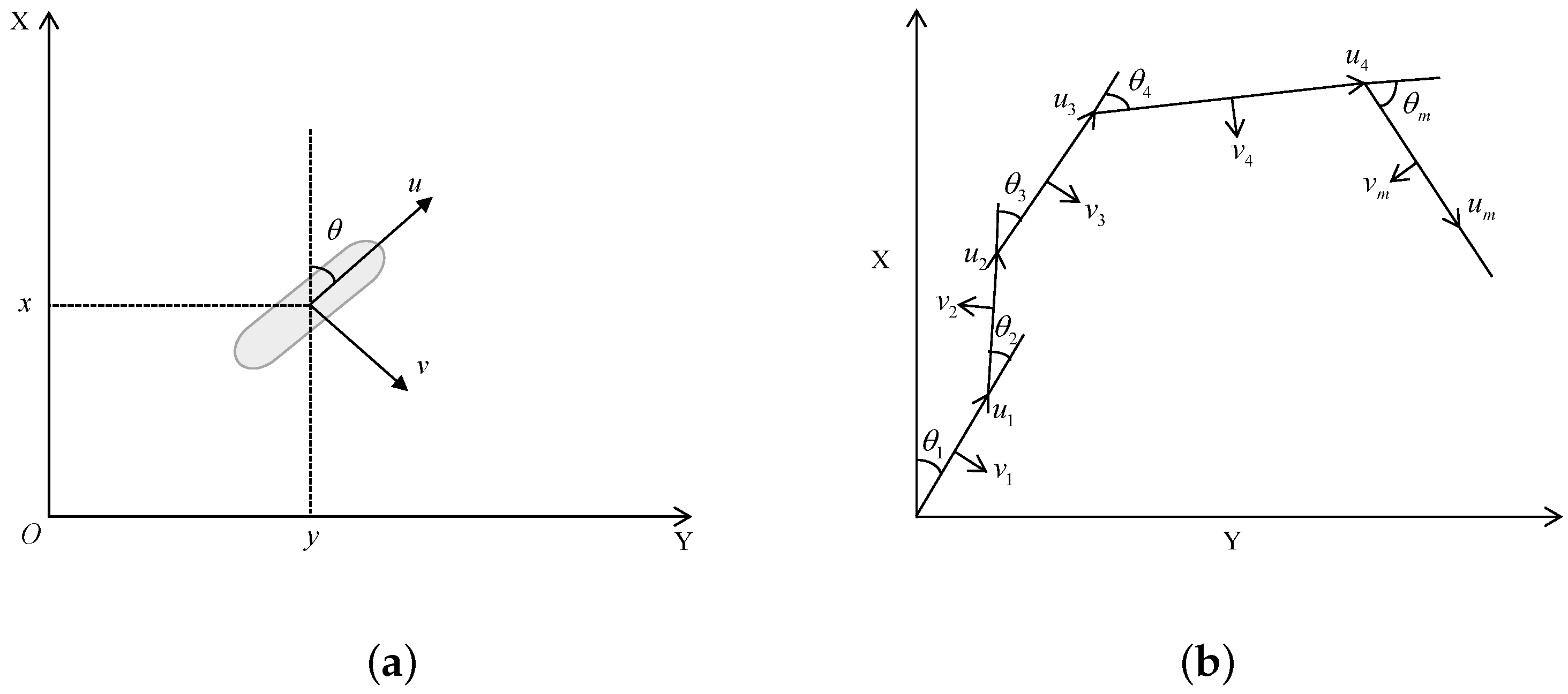
This study aims to quantitatively analyze the growth of errors over time or distance through numerical error analysis. To simplify the problem description, an AUV is assumed to move at a fixed depth in a Cartesian coordinate system, which aligns with its actual navigation mode. A typical 3-DOF motion model is utilized to accurately present the AUV’s dynamic characteristics and precisely calculate the ego-motion vector.
Figure 1a shows the proposed motion model. The relationship between relative attitude measurements and the position, as established with the AUV model, is depicted in
Figure 1b. The figure illustrates the relationship between relative attitude measurements and the position of the AUV model, where
and
represent the frame number and measurement value, respectively. In the case of consecutive frames,
represents the heading angle, and
u and
v represent two speeds: the forward velocity and transverse velocity. The specific parameter definitions are shown in
Table 1. We define the pose measurements
,
, and
as true values.
,
, and
are noise errors. Assuming that they are independent, the mean and standard deviation of
,
, and
are zero. Therefore, the measured values of each step are shown as follows when the measured values of the relative attitude, true values, and errors are determined:
where corresponding errors are I.I.D. The position is calculated with
The accumulation of drift in noise measurements is unbounded. While the Cramer–Rao theory can be used to estimate lower bounds, traditional methods fail to estimate upper bounds, especially in the absence of fundamental assumptions. However, statistical estimation of errors can be accomplished by analyzing the error distribution characteristics of multiple statistics.
2.2. True Error Statistics
Based on the aforementioned assumptions, a specific kinematic model can be employed to simulate AUV positioning and dead-reckoning errors in continuous frames. This kinematic model correlates the AUV’s position and velocity with time, enabling us to predict the position and orientation in each frame. By comparing the predicted results from consecutive frames with actual measurements, we can estimate dead-reckoning errors and further analyze their cumulative trend over time. This extended approach provides an effective means of understanding a AUV’s localization performance in autonomous underwater navigation and its response to different motion patterns and measurement conditions.
where
and
represent the true value, and
and
represent the error value.
and
are the ground-truth positions.
After obtaining the extended formulation for the actual vehicle position, we can derive the expression for the error values.
By utilizing the aforementioned formulas, we can calculate the expected value and variance of the cumulative error. It is important to note that each stepwise error is correlated with the actual attitude measurements. For analytical purposes, we make the assumption that the errors follow a zero-mean Gaussian distribution with a certain variance. This facilitates further analysis of the behavior of the cumulative error, as it is related to the motion and measurement uncertainties of the AUV.
Assuming that
,
and
, we can obtain mathematical statistics for the following expressions:
Once the above formula has been obtained, the expected value of the sine and cosine can be calculated to simplify the subsequent formula’s calculation:
Then, we need to separately take the expectations of
and
. By substituting Equation (
8) into the expression for
and
and simplifying, their respective expected values can be obtained:
The above equation gives the first-order distance. By combining it with the Cauchy–Schwarz inequality, we can obtain the second moment:
Since the calculation method for the second moment of cumulative error in the
X direction is the same as that in the
Y direction, we will focus on demonstrating the calculation process for
X. In the subsequent analysis, we will further simplify this expression. Based on the aforementioned equation, we obtain:
Through calculations, we can obtain the preliminary expression for the second moment of cumulative error on the
X axis. It consists of four components but has not been fully simplified. To further simplify this expression, we will apply the Cauchy–Schwarz inequality.
Finally, we combine the four parts of the simplification, and
becomes
In the same way, we can calculate the second-order moment of the cumulative error in the
Y direction. The specific expression of the second moment is shown below:
2.3. Error Statistics in Practice
Based on the AUV’s kinematic model, we derived the expression of the second moment for cumulative errors in the two-dimensional direction. However, these expressions cannot be used directly because they require the actual values of the arguments. In reality, it is not possible to obtain the actual values, and we can only obtain relative attitude measurements with noise. Therefore, the real expected value is determined based on the actual measurements in order for the results to be useful.
To obtain the actual expected value, we can extend the previous equation by using Equation (
1). In this process, we replace the relative attitude measurements with the actual values. Specifically, we calculate
to obtain the actual values while taking the influence of real attitude measurement errors on the cumulative errors into account.
Building upon the first moment of the cumulative error, we can derive the second moment of the cumulative error by using the Cauchy–Schwarz inequality. The details are as follows:
After obtaining the above calculation results, we need to continue to simplify
:
As shown in Equations (
22) and (25), we obtained the expectation and variance of the cumulative error in the
X direction. By following the same calculation procedure, we can compute the statistical properties of the cumulative error in the
Y direction.
After performing the necessary computations, we obtained the expected value and variance of the cumulative error. In the calculation process, we first derived the statistical characteristics of the cumulative error based on actual values, although such data are not directly accessible in the real world. However, by substituting parameters, we were able to complete the calculations and obtain the properties of the cumulative error that depend on actual values and errors. It is important to note that despite simplifications, the resulting expressions remain quite complex.
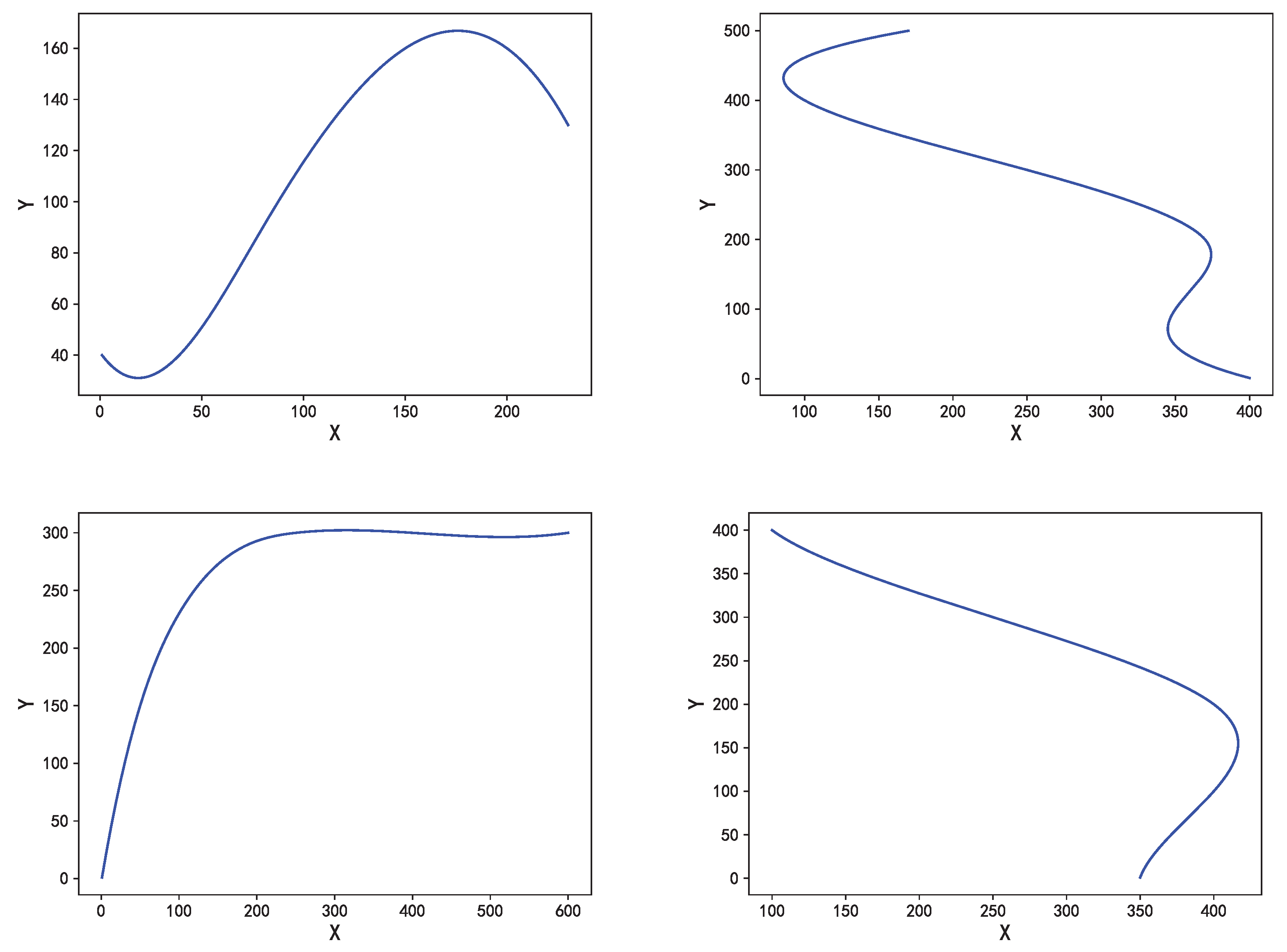
To verify the accuracy of our formulas, we need to set up four trajectories and determine the level of noise that is present. We employed Monte Carlo simulations to compare the statistical properties obtained from the simulations with the results of our formula calculations. Through this validation method, we can ensure that our model accurately describes the behavior of cumulative errors under real-world conditions.
3. Experimental Results
To assess the statistical properties of underwater dead reckoning, we conducted Monte Carlo simulations, which involved multiple measurements of the same scenario to demonstrate the randomness of errors. In each simulation, we generated multiple sets of noisy measurements for each trajectory and used them to estimate the expected value and variance of the cumulative error. By repeating this process several times, we obtained statistical characteristics that reflected the behavior of underwater dead reckoning under different noise conditions. Unlike typical autonomous driving datasets, our proposed dataset includes global positions and internal measurements in underwater scenarios with noise that was manually added to the relative measurements of the ground truth.
The forward velocity noise, transverse velocity noise, and heading angle noise were considered as 0.1 m, 0.1 m, and 0.005 rad, respectively, as shown in
Table 2.
Figure 2 displays the four original trajectories calculated with the ground-truth values.
During the simulation process, the evaluation of the first moment of underwater localization errors was carried out by using the following method (taking the
X direction as an example). The same approach is also applicable to the evaluation of the first moment in the
Y direction. By repeating the simulations and calculations, robust first-moment assessments under different noise conditions were obtained, providing a clear understanding of the variation trend of cumulative errors in underwater positioning.
Figure 3,
Figure 4,
Figure 5,
Figure 6,
Figure 7,
Figure 8,
Figure 9 and
Figure 10 show the results of the Monte Carlo simulation for the estimated underwater localization error.
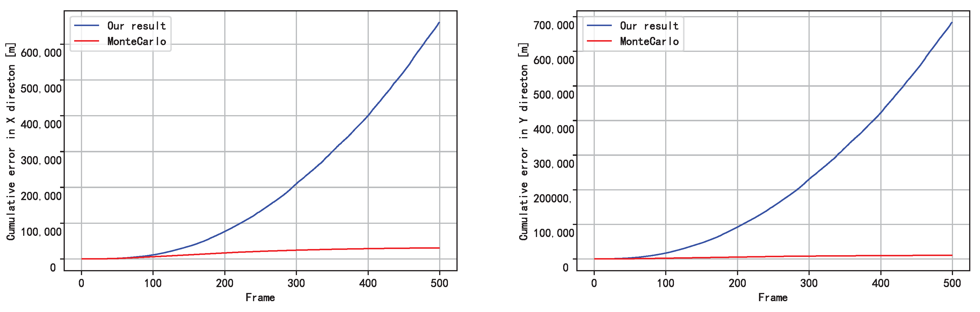
Figure 3,
Figure 4,
Figure 5 and
Figure 6 present the expected values, while
Figure 7,
Figure 8,
Figure 9 and
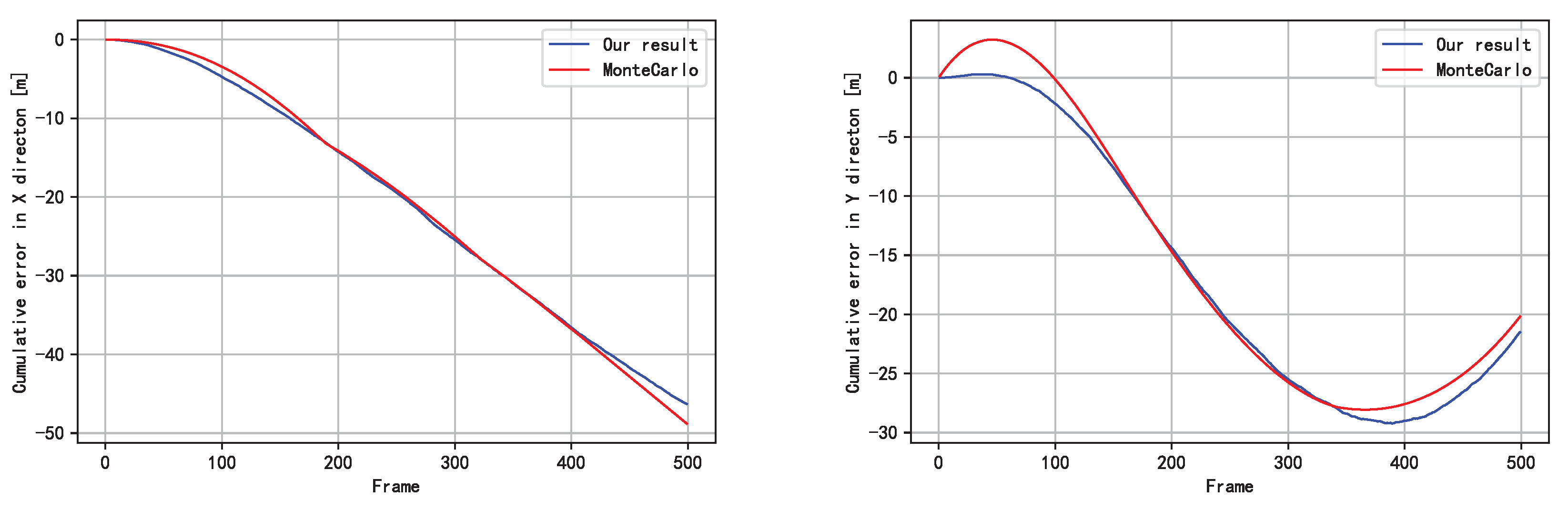
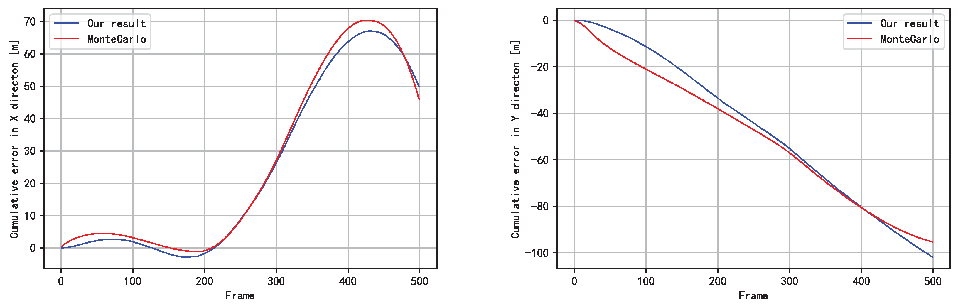
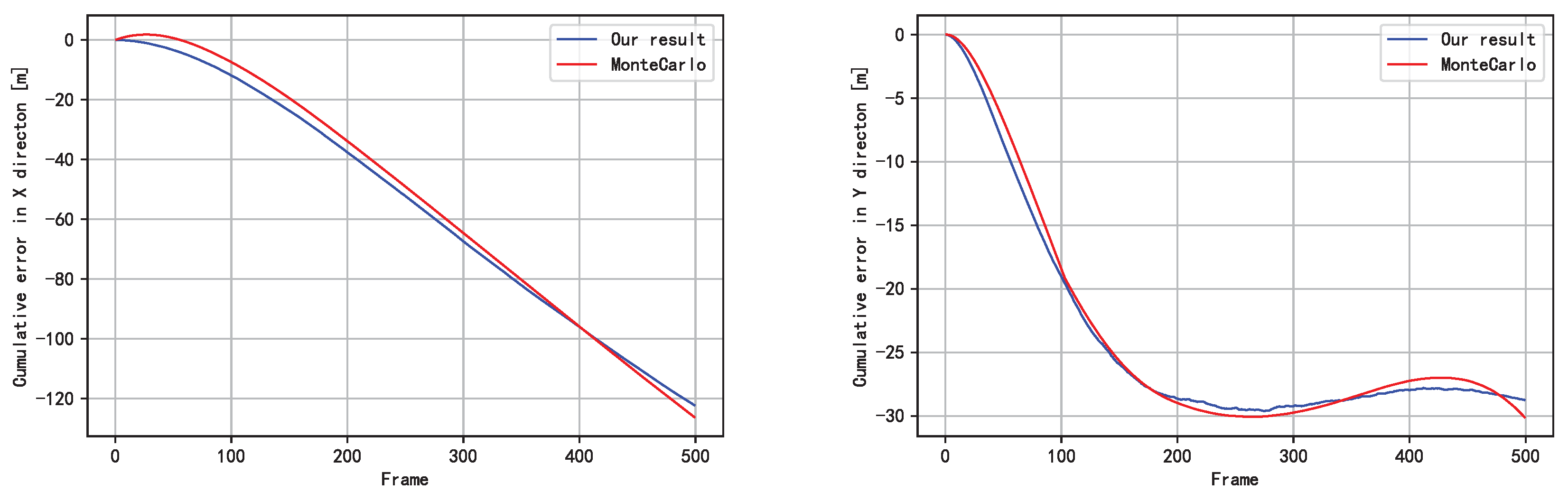
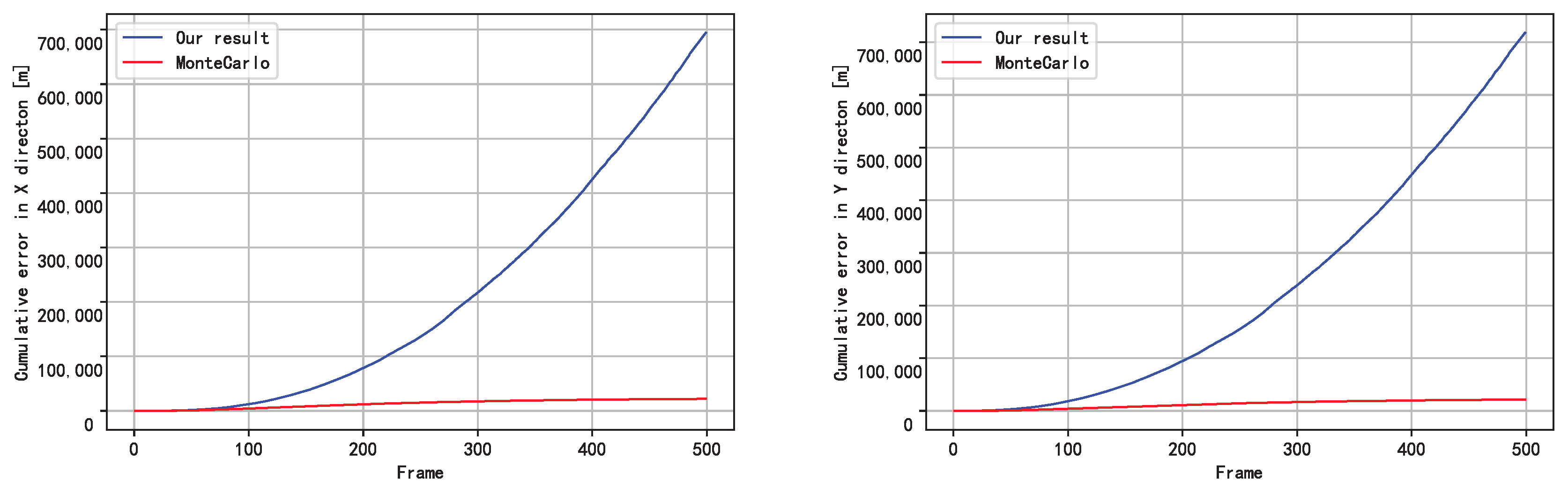
Figure 10 present the corresponding variances. In these figures, the red lines represent the evaluation results from the Monte Carlo simulations, while the blue lines represent our theoretical results. It can be observed that the estimated first-order moments were very close to the actual errors in the Monte Carlo simulations, while the variances were higher.
In
Figure 3 and
Figure 7, we present the first and second moments of trajectory 1. As shown in
Figure 2a, the AUV followed a curved path, leading to a continuous increase in the
X-direction error and a fluctuating
Y-direction error. The observed variations in these values aligned with the vehicle’s motion, which was mainly due to the nonlinear nature of the second moment. In real-world underwater positioning scenarios, a AUV’s motion trajectories can be highly complex, resulting in varying performance of the accumulated error. This nonlinear behavior significantly impacts the accuracy and stability of the positioning, and, generally, simpler trajectories tend to result in lower positioning errors. As a result, it is essential to consider the influence of trajectory complexity when designing and optimizing underwater positioning systems.
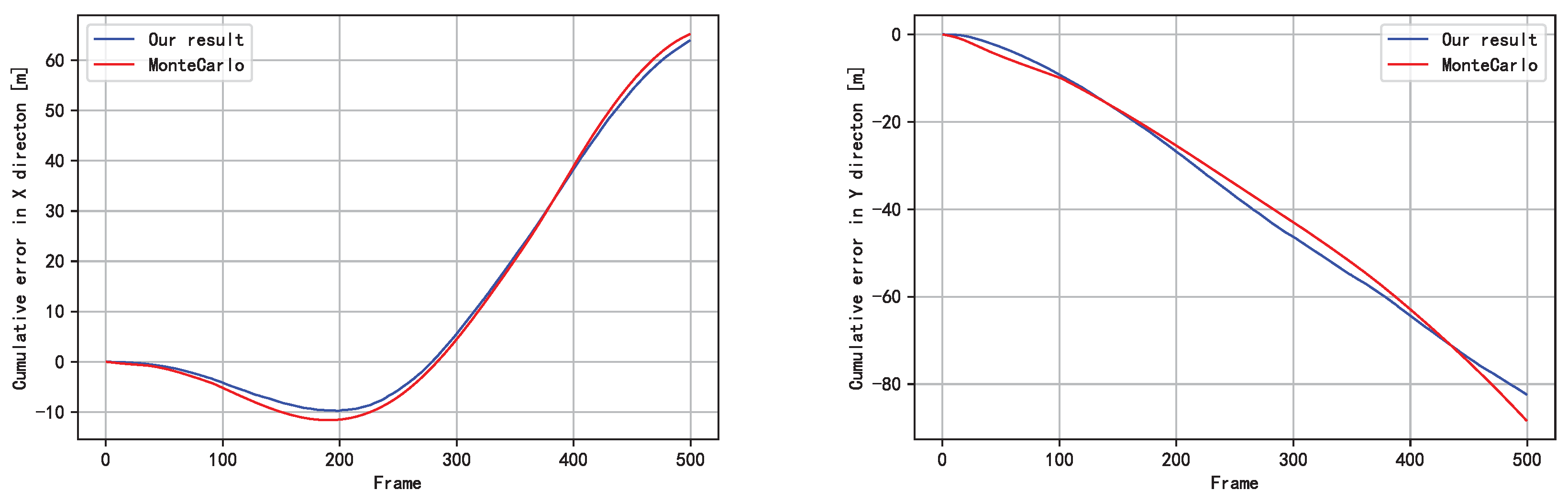
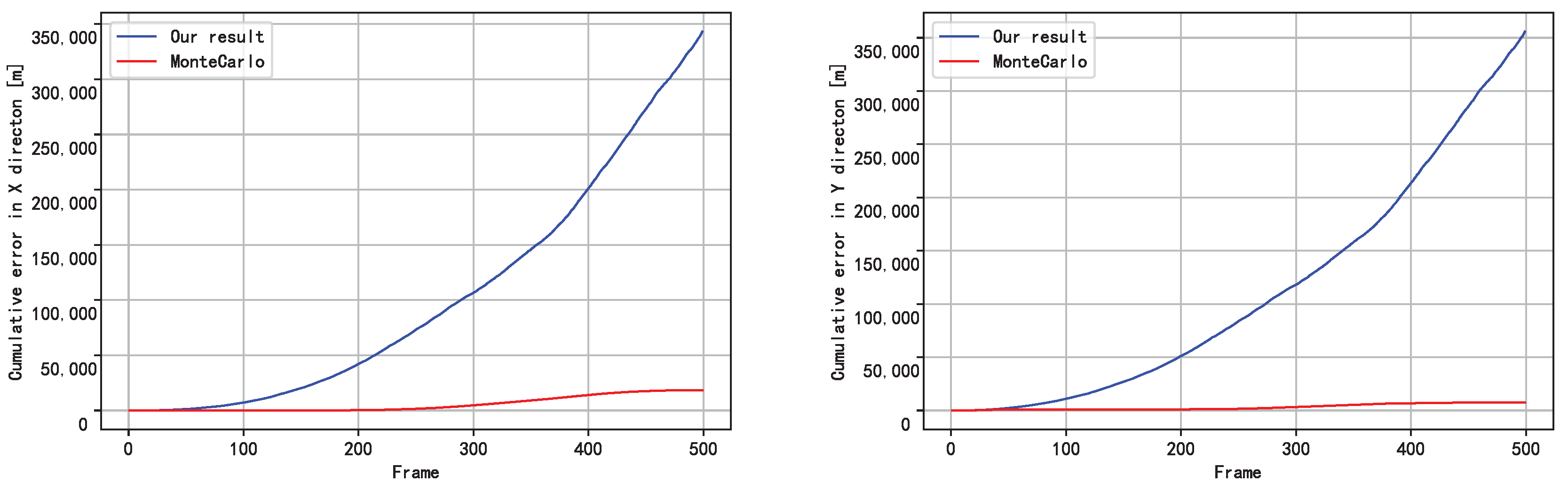
Similarly,
Figure 4 and
Figure 8 present the corresponding results for trajectory 2. Unlike in the previous scenario, the underwater vehicle followed a circular path in this case, and the estimated results exhibited patterns consistent with its motion. However, we observed that the estimation of the second moment was consistently inaccurate. The circular path introduced periodicity in the AUV’s motion along the
X and
Y directions, leading to more complex and unstable estimates of the second moment. This indicated that when the AUV’s motion trajectory possessed more nonlinear features, the accuracy of the cumulative error was challenged, thereby increasing the risk and difficulty of localization.
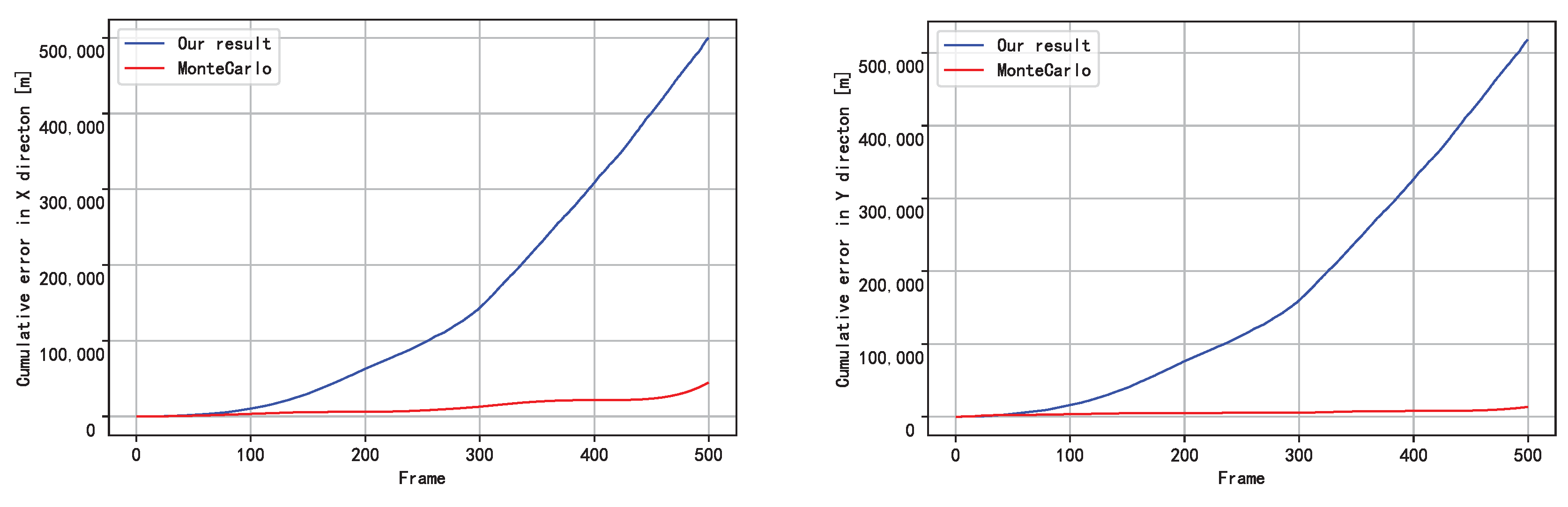
The experimental results demonstrate a strong agreement between the cumulative error model and the statistical characteristics, particularly in the first order. Our proposed model accurately fits the expected statistical properties, indicating its high robustness throughout the process without actual measurements, thus providing a mathematical solution for evaluating attitude measurements based on relative errors. However, as the distance becomes sufficiently large, the growth rate of variance becomes unbounded, resulting in significant degradation of the performance in the second order. Nevertheless, it can still be considered an online solution for underwater navigation applications. To further explore how to improve the performance in the second order by introducing additional information or utilizing prior knowledge and, thereby, to enhance the accuracy and stability of underwater navigation, we conducted further evaluations.
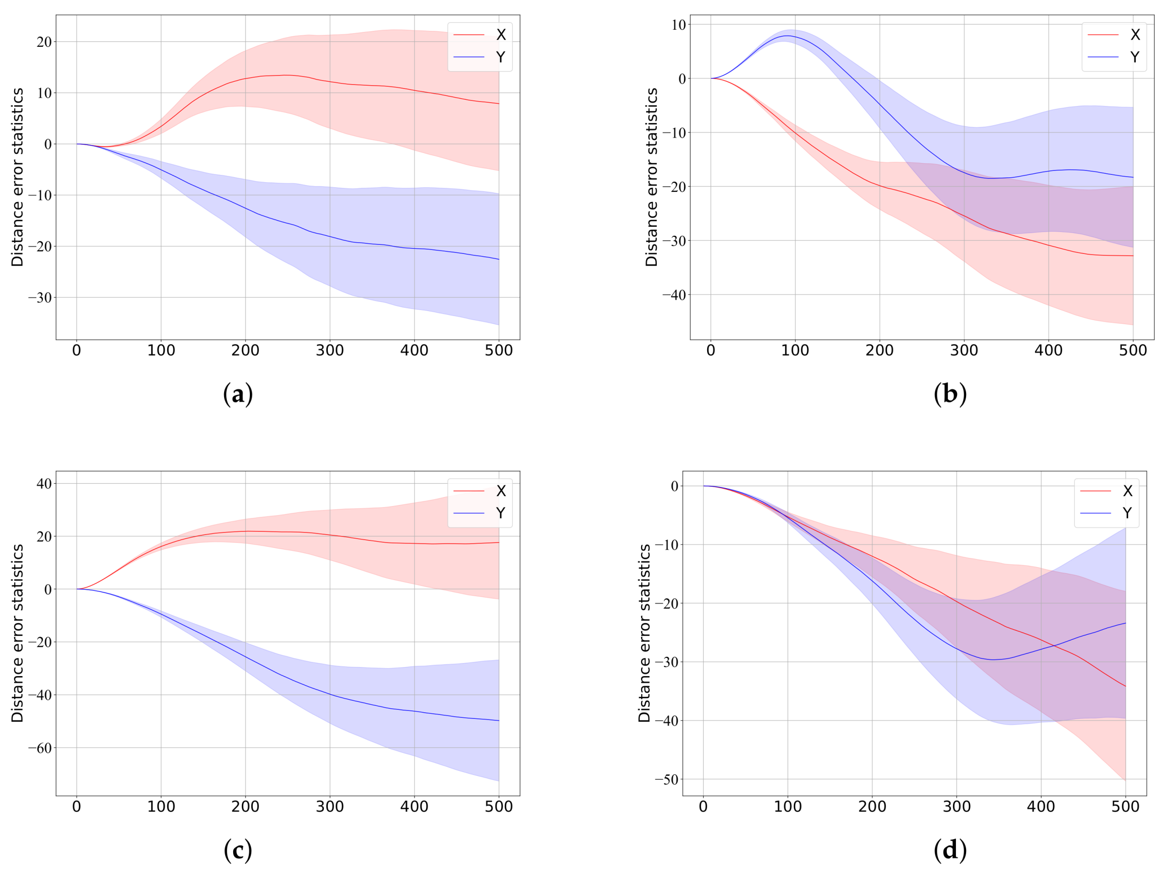
Figure 11 and
Figure 12 display the Monte Carlo results of the estimated underwater localization error uncertainty. As shown in
Figure 11, the growth trend of the error expectation from multiple tests was consistent with that of our method, and the uncertainty in error variation grew moderately, although the effect was not significant. This confirmed the accuracy of our method.
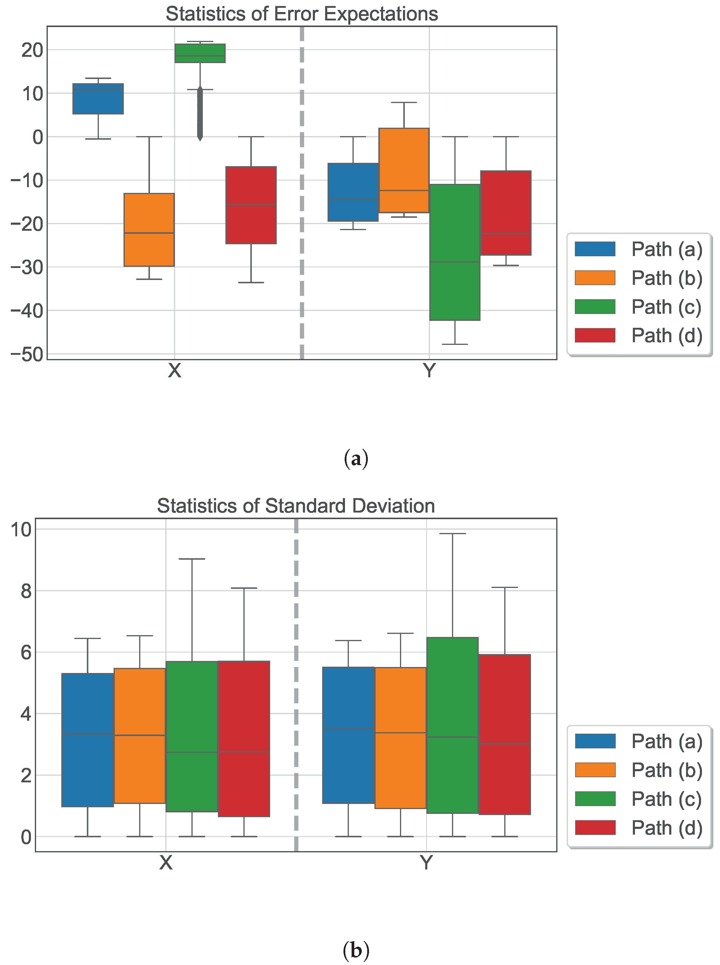
To provide a quantitative and intuitive observation,
Figure 12 presents the statistics of multiple results, showing that the uncertainty in the error remained stable. The expectation in the
X and
Y directions under different trajectories was influenced by the trajectory trends, but more complex trajectories did not result in significantly higher uncertainty. It is worth noting that trajectory
c generated additional outliers in the expectation, which was speculated to be caused by uncertain errors arising from straight trajectories.
Furthermore, the uncertainty in the error variance was relatively low across different trajectories, indicating that our method effectively accounted for the error variations. The obtained results highlight the robustness and reliability of our proposed method in addressing uncertainties related to underwater localization errors, particularly when dealing with complex and diverse trajectories. The stability of error uncertainty under different conditions demonstrates the effectiveness of our method in providing accurate and consistent estimates for underwater navigation methods.
4. Conclusions and Discussion
We proposed a noise-based internal measurement odometry uncertainty modeling method for underwater navigation that was specifically designed to mitigate the drift effects of cumulative errors in acoustic-denied environments. To address this challenge, we approximated the first two moments of the cumulative errors. In comparison to related approaches, our method does not rely on fundamental assumptions but, rather, recursively estimates biases and uncertainties, thus yielding empirical formulas with statistical characteristics. Through Monte Carlo simulations in various underwater navigation scenarios, we validated the effectiveness and robustness of the proposed modeling approach. The experimental results demonstrate that our formulas significantly reduce errors in odometry, particularly excelling in eliminating cumulative errors in complex environments.
Our model may also have great potential in the following areas:
The mathematical model that we proposed, in combination with the RFID-based range measurement method, holds great potential. Odometer systems typically require recalibration of the position through reference points to mitigate the cumulative error. Our model represents the first moment of the cumulative error accurately, and it does not require truth values. Hence, it is feasible to use our model to calculate the optimal distribution of reference sensors throughout the process. This method can provide a mathematical solution for the optimal distribution of RFID sensors in large-scale environments.
The evaluation of the performance of various range methods in a large-scale environment is a challenging task, as different trajectories can result in deviations from the actual state. In this paper, we proposed a mathematical solution for calculating the statistics of cumulative errors, and this can serve as a natural bridge for evaluating the corresponding performance.
Of course, further research could be conducted to expand the scope of the study. For instance, in some underwater missions, the vehicle may need to carry out three-dimensional motion, which involves tasks at different depths. However, this work primarily focused on the statistical characteristics of cumulative errors at the same horizontal level based on three degrees of freedom. To address this limitation, future studies could establish a six-degree-of-freedom motion model of the vehicle and obtain the statistical characteristics of the cumulative errors during three-dimensional motion.


