Self-Interference Suppression of Unmanned Underwater Vehicle with Vector Hydrophone Array Based on an Improved Autoencoder

Abstract

The self-interference of an unmanned underwater vehicle (UUV) weakens its ability to detect targets of interest. Due to limitations in the size of the sonar array and the complexity of the interference, the performance of existing self-interference suppression methods in practical applications is unsatisfactory. Our research focuses on analyzing the influence of near-field interferences on the sample covariance matrix (SCM) and proposes an interference suppression algorithm based on an improved autoencoder. The proposed algorithm effectively learns the feature distribution of near-field interferences within the covariance domain and reconstructs the pure signal covariance matrix through the cancellation of the near-field interference features. Moreover, the proposed algorithm can meet the requirements of real-time processing and does not require prior knowledge about the positions or propagation of interference. Simulations demonstrate that the proposed algorithm outperforms comparison methods, particularly in scenarios with low signal-to-interference ratios and a limited number of sensors. Furthermore, lake experiments provide additional evidence of the proposed algorithm’s good performance in practical applications.

1. Introduction

In recent times, UUVs have gained substantial attention for their mobility, concealment, and low energy consumption in applications such as underwater target reconnaissance, ocean environment detection, and maritime rescue. As the development of stealth technology for underwater targets has led to a reduction in radiation noise levels, it has become crucial to enhance the underwater target detection range of UUVs [1]. To achieve this, UUVs are typically equipped with flank sonar arrays on both sides, as they provide a larger array aperture compared to a head sonar. This allows for a lower operating frequency and a greater detection range. However, when UUVs are in high-speed motion, they produce strong self-interference, which is considered to be near-field interference. The self-interference decreases the UUV’s detection ability for weak targets in the far field. Thus, the development of UUV self-interference suppression technology has become an urgent necessity for improving its performance.

Self-interference suppression poses a critical challenge for UUVs, leading researchers to explore various techniques to address this issue. These techniques can be categorized into adaptive interference cancellation [2,3], focused-beamforming-based interference cancellation [4,5,6], and spatial-filtering-based interference cancellation [7,8,9,10,11]. Gao et al. [3] have employed an adaptive filtering method to cancel correlated noise of sonar arrays by extracting reference noise with a multi-channel difference method. However, this algorithm heavily relies on the accuracy of reference signal estimation, and its performance is limited in complex marine environments. Focused beamforming, on the other hand, is capable of handling near-field spherical waves and estimating the location of near-field sources, which makes it an invaluable tool for near-field interference suppression. In the study by Ref. [4], an interference suppression method based on nulling weight of a near-field focused beam is proposed, which demonstrates suitability for practical applications due to its relatively low computational complexity. Nonetheless, the effectiveness of this method greatly depends on the precise estimation of the interference’s position. Ning et al. [6] introduced a real-time interference suppression algorithm for mitigating tail self-interference in underwater vehicles using adaptive focused inverse beamforming. The tail self-interference can be estimated by focused beamforming and suppressed by the inverse operation at each sensor. Spatial-filtering-based interference cancellation techniques often utilize matrix filtering algorithms, which are primarily designed to suppress signals from a specific sector while allowing signals from other sectors to pass through. Liang et al. [9] extended the matrix filter algorithm to address near-field interference suppression of underwater platforms. This method divides a passband and a stopband in the far and near field, respectively, and suppresses the interference components in the near-field stopband by solving the filtering matrix. Simulation results demonstrate its excellent interference suppression capabilities. However, the efficacy of the filter is contingent upon the relative position of the near and far field source, which may result in varying degrees of distortion for signals of interest.

In the past five years, deep learning methods have demonstrated promising performance in underwater target localization [12,13,14,15,16,17] and direction-of-arrival estimation [18,19,20,21,22]. Deep learning algorithms are good at finding solutions to problems from big data, giving it an advantage over traditional methods. When tackling challenging problems in underwater acoustics, traditional methods rely on constructing physical models to gain a better understanding of the acoustic phenomena [23]. However, it is always challenging to construct a physical model which can accurately capture and explain the corresponding highly complex acoustic phenomena.

Facing the problems of underwater platform interference suppression, the current methods have some degree of idealization as they oversimplify the intricate coupling relationship between the interference and the signal. To the best of our knowledge, we are the first to apply deep learning to the field of interference suppression of underwater platforms for potential performance improvement. An improved autoencoder is introduced to suppress self-interference of underwater vehicles. In our paper, the influence of near-field interference on the array covariance matrix is analyzed, and the proposed autoencoder algorithm is introduced to suppress the interference in the feature domain. Subsequently, a set of simulation parameters is established to evaluate the performance of the proposed method. Furthermore, a lake experiment is conducted to further validate its effectiveness.

The remainder of this paper is organized as follows: Section 2 presents the formulation of the vector array receiving model. Section 3 introduces an improved autoencoder model and explains of its functionality for interference suppression. Section 4 conducts simulations to demonstrate the superiority of the proposed method compared to other comparison methods. Section 5 verifies the effectiveness of the proposed algorithm by a lake experiment. Section 6 presents the conclusion of this paper.

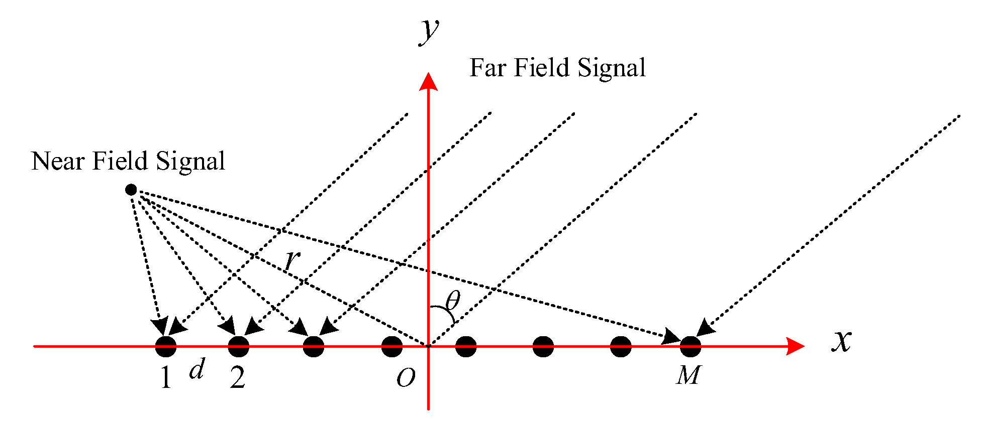
2. Vector Array Receiving Model

Suppose that a uniform linear array (ULA) consisting of $M$ sensors is the flank sonar array of a UUV. Figure 1 illustrates the array receiving model of a uniform linear array. The center of the linear array is designated as the origin for both the Cartesian and polar coordinate systems for describing both far-field and near-field signals conveniently. See

Table 1. Explanations of some variables and symbols through this paper.

Symbol	Definition	Cardinality
Signal model
$(r_i,{\theta }_i)$	Near-field location of polar coordinate
$p_m(t)$	The received waveform of the mth sensor
$s_k(t)$	The kth source’s waveform at reference position
${\mathit{A}}_S(\theta )$	Array manifold of far-field signal	${ℂ}^{M_v\times Q_1}$
${\mathit{A}}_I(r,\theta )$	Array manifold of near-field signal	${ℂ}^{M_v\times Q_2}$
$\mathit{X}(t)$	Matrix of receiving data of vector array
$M$	Total number of sensors
$M_v$	Total number of channels
${\mathit{R}}_x$	Covariance matrix	${ℂ}^{M_v\times M_v}$
${\tilde{\mathit{R}}}_x$	Sample covariance matrix (SCM)	${ℂ}^{M_v\times M_v}$
$T_S$	Snapshot number
Data preprocessing
$\tilde{\mathit{C}}(\omega )$	Frequency cross-spectral matrix	${ℂ}^{M_v\times M_v}$
$\mathit{U}$	DIAE input: Vectorized covariance matrix	${ℝ}^{(M_v+1)M_v}$
$\mathit{T}$	DIAE label	${ℝ}^{(M_v+1)M_v}$
$fv(·)$,$ifv(·)$	Vectorization transformation and its inverse operation
${\mathit{C}}_S$,${\mathit{C}}_I$	Far-field target and near-field interference feature
DOA
${\delta }^2{}_{\mathrm{CBF}}(\theta )$	CBF output at candidate angle $\theta$
$G$	Filter matrix	${ℂ}^{M_v\times M_v}$
${\mathrm{\Theta }}_P=\left\{{\theta }_i\right|i=1,\dots ,P\}$	Passband in matrix filter
${\mathrm{\Theta }}_S=\{(r_i,{\theta }_i),|i=1,\cdots ,S\}$	Stopband in matrix filter

for symbols and definitions used throughout this paper.

For an underwater sound signal located at $(r_i,{\theta }_i)$, the target is usually defined as a far-field source when the distance between the target and the array satisfies the following formula:

$$r_i\gg \frac{{\left[(M-1)d\right]}^2}{\lambda },$$

(1)

• $\lambda$: the signal wave length;
• $(M-1)d$: the array aperture with the sensor spacing as $d$.

The wavefront of acoustic propagation is regarded as a plane for far-field signals, whereas, for near-field signals, it is considered to be spherical. Assume that the target of interest are Q₁-independent far-field signals, impinging onto the hydrophone array with incident directions $[{\theta }_1,{\theta }_2,\dots ,{\theta }_{Q_1}]$. The interference comprises Q₂-independent near-field signals impinging from positions $[(r_1,{\theta }_1),(r_2,{\theta }_2),\dots ,(r_{Q_2},{\theta }_{Q_2})]$. The received waveform of the mth sensor is $p_m(t)$ and can be formulated as follows [24]:

$$p_m(t)={\displaystyle \sum _{k=1}^{Q_1}{s}_k(t-{\tau }_{mk})}+{\displaystyle \sum _{k=Q_1+1}^{Q_1+Q_2}{\beta }_k\frac{r_k}{r_{mk}}{s}_k(t-{\tau }_{mk})}+n_m(t),m=1,2,\dots ,M,$$

(2)

• $n_m(t)$: the additive zero-mean Gaussian noise;
• ${\tau }_{mk}$: the time delay of source $k$ between mth sensor and the reference position;
• $r_{mk}$: the distance between near-field source $k$ and the mth sensor;
• $r_k$: the distance between near-field source $k$ and the reference position.

The near-field signal propagates in a spherical waveform, resulting in the attenuation of waveform amplitude, and $r_k/r_{mk}$ is the amplitude attenuation associate with source $k$ at mth sensor relative to the reference position. The received signal $p_m(t)$ is the mth sensor waveform measured in units of sound pressure, and as a vector hydrophone it is capable of simultaneous measurements of both sound pressure $p$ and vibration velocity $v$. Equation (3) denotes the relationship between sound pressure and vibration velocity of a plane wave, with $\rho$ representing the density of water and $c$ denoting the sound speed.

$$\frac{p(t)}{v(t)}=\rho c.$$

(3)

For plane waves, sound pressure and vibration velocity are in phase. Near-field source propagates in the form of spherical waves, and the sound pressure and velocity satisfy as follows [25]:

$$\frac{p(t,r)}{v(t,r)}=\frac{\rho c}{1-j\frac{\lambda }{2\pi r}}.$$

(4)

The imaginary part $\lambda /2\pi r$ in the denominator cannot be ignored under near-field conditions. In other words, there is a phase difference between the sound pressure and the velocity in spherical waveform. The vibration velocity $v$ can be decomposed into two orthogonal channels $v_x,v_y$. Omitting the acoustic impedance $\rho c$, the direction vector of a plane wave at a single vector sensor can be expressed as:

$$[p,v_x,v_y]={\left[1,\cos \theta ,\sin \theta \right]}^{\mathrm{T}},$$

(5)

• $\theta$: the azimuth of the vibration velocity relative to the x-axis direction.

Likewise, the direction vector of a spherical wave at a single vector sensor can be expressed as:

$$[p,v_x,v_y]={\left[1,(1-j\lambda /2\pi r)\cos \theta ,(1-j\lambda /2\pi r)\sin \theta \right]}^{\mathrm{T}}.$$

(6)

Let ${\mathit{s}}_S(t)$ and ${\mathit{s}}_I(t)$ denote far-field signals and near-field interference, respectively. The receiving data of the vector array can be written in matrix form:

$$\mathit{X}(t)=\left[{\mathit{A}}_S(\theta ){\mathit{A}}_I(r,\theta )\right] \left[\begin{array}{l}{\mathit{s}}_S(t)\\ {\mathit{s}}_I(t)\end{array}\right]+\mathit{N}(t),$$

(7)

• ${\mathit{A}}_S(\theta )$: $[{\mathit{a}}_S({\theta }_1),\dots ,{\mathit{a}}_S({\theta }_{Q_1})]\in {ℂ}^{3M\times Q_1}$;
• ${\mathit{A}}_I(r,\theta )$: $[{\mathit{a}}_I(r_{Q_1+1},{\theta }_{Q_1+1}),\dots ,{\mathit{a}}_I(r_{Q_1+Q_2},{\theta }_{Q_1+Q_2})]\in {ℂ}^{3M\times Q_2}$;
• ${\mathit{s}}_S(t)$: ${[s_1(t),s_2(t),\dots ,s_{Q_1}(t)]}^{\mathrm{T}}$;
• ${\mathit{s}}_I(t)$: ${[s_{Q_1+1}(t),s_{P+2}(t),\dots ,s_{Q_1+Q_2}(t)]}^{\mathrm{T}}$.

Each column of ${\mathit{A}}_S(\theta )$ and ${\mathit{A}}_I(r,\theta )$ is a steering vector, denoted by

$$\begin{array}{cc}{a}_S({\theta }_i)=& {\left[1,\exp \left(-j\frac{2\pi d\cos {\theta }_i}{\lambda }\right),\dots ,\exp \left(-j\frac{2\pi (M-1)d\cos {\theta }_i}{\lambda }\right)\right]}^{\mathrm{T}}\otimes {\left[1,\cos {\theta }_i,\sin {\theta }_i\right]}^{\mathrm{T}}\\ a_I(r_i,{\theta }_i)=& {\left\{\begin{array}{c}1\otimes \left[1,\left(1-j\frac{\lambda }{2\pi r_{1i}}\right)\cos {\theta }_{1i},\left(1-j\frac{\lambda }{2\pi r_{1i}}\right)\sin {\theta }_{1i}\right],\\ \frac{r_i}{r_{2i}}\exp \left(j\frac{2\pi \left(r_i-r_{2i}\right)}{\lambda }\right)\otimes \left[1,\left(1-j\frac{\lambda }{2\pi r_{2i}}\right)\cos {\theta }_{2i},\left(1-j\frac{\lambda }{2\pi r_{2i}}\right)\sin {\theta }_{2i}\right],\dots ,\\ \frac{r_i}{r_{Mi}}\exp \left(j\frac{2\pi \left(r_i-r_{Mi}\right)}{\lambda }\right)\otimes \left[1,\left(1-j\frac{\lambda }{2\pi r_{Mi}}\right)\cos {\theta }_{Mi},\left(1-j\frac{\lambda }{2\pi r_{Mi}}\right)\sin {\theta }_{Mi}\right]\end{array}\right\}}^T\end{array}$$

(8)

• $\otimes$: the Kronecker product operator.

Array signal processing algorithms usually focus on the statistical characteristics of array signals, and the covariance matrix can be expressed as

$${\mathit{R}}_x=\mathrm{E}\left\{\mathit{X}(t)\mathit{X}{(t)}^{\mathrm{H}}\right\}.$$

(9)

In practical applications, the sample covariance matrix (SCM) ${\tilde{\mathit{R}}}_x$ is used to approximate ${\mathit{R}}_x$, which is denoted by:

$${\tilde{\mathit{R}}}_x=\frac{1}{T_s}{\displaystyle {\sum }_{t=1}^{T_s}\left\{\mathit{x}(t)\mathit{x}{(t)}^{\mathrm{H}}\right\}},$$

(10)

• $T_s$: the number of snapshots.

When there is no near-field interference, i.e., $\mathit{\beta }=({\beta }_{Q_1+1},\dots ,{\beta }_{Q_1+Q_2})=\mathbf{0}$,

$${\tilde{\mathit{R}}}_x=\frac{1}{T_s}{\displaystyle {\sum }_{t=1}^{T_s}\left\{\left[{\mathit{A}}_S(\theta ){\mathit{s}}_S(t)+\mathit{n}(t)\right]·{\left[{\mathit{A}}_S(\theta ){\mathit{s}}_S(t)+\mathit{n}(t)\right]}^{\mathrm{H}}\right\}}.$$

(11)

Otherwise, when near-field interference exists, i.e., $\mathit{\beta }=({\beta }_{Q_1+1},\dots ,{\beta }_{Q_1+Q_2})=\mathbf{1}$,

$${\tilde{\mathit{R}}}_x{}^{\prime }=\frac{1}{T_s}{\displaystyle {\sum }_{t=1}^{T_s}\left\{\begin{array}{l}\left[{\mathit{A}}_S(\theta ){\mathit{s}}_S(t)+{\mathit{A}}_I(\theta ){\mathit{s}}_I(t)+\mathit{n}(t)\right]·\\ {\left[{\mathit{A}}_S(\theta ){\mathit{s}}_S(t)+{\mathit{A}}_I(\theta ){\mathit{s}}_I(t)+\mathit{n}(t)\right]}^{\mathrm{H}}\end{array}\right\}}.$$

(12)

Assume that signal, interference, and noise are not correlated in pairs; $\mathrm{\Delta }{\tilde{\mathit{R}}}_x$ represents the increment on the SCM caused by near-field interference source, which can be expressed as:

$$\begin{array}{cc}\mathrm{\Delta }{\tilde{\mathit{R}}}_x& ={\tilde{\mathit{R}}}_x{}^{\prime }-{\tilde{\mathit{R}}}_x\hfill \\ & \approx \frac{1}{T_s}{\displaystyle {\sum }_{t=1}^{T_s}\left\{{\mathit{A}}_I(\theta )s_I(t)s_I{(t)}^{\mathrm{H}}{\mathit{A}}_I{(\theta )}^{\mathrm{H}}\right\}} \hfill \\ & ={\mathit{A}}_I(\theta ){\tilde{\mathit{R}}}_I{\mathit{A}}_I{(\theta )}^{\mathrm{H}}\hfill \end{array}$$

(13)

• ${\tilde{\mathit{R}}}_I=\frac{1}{T_s}{\displaystyle {\sum }_{t=1}^{T_s}\left\{s_I(t)s_I{(t)}^{\mathrm{H}}\right\}}$.

It is imperative to note that treating the self-interference of a UUV as multiple independent near-field sources is merely a simplification, as the underlying mechanism behind its generation is a highly intricate process. Both the real array manifolds ${\mathit{A}}_I(\theta )$ and covariance matrix ${\tilde{\mathit{R}}}_I$ of interference are difficult to obtain; in other words, $\mathrm{\Delta }{\tilde{\mathit{R}}}_x$ cannot be accurately estimated by Equation (13). Based on the above analysis, we propose a near-field interference suppression algorithm based on an autoencoder model, which can suppress the $\mathrm{\Delta }{\tilde{\mathit{R}}}_x$ component in the feature domain. The algorithm does not need to estimate ${\mathit{A}}_I(\theta )$ or ${\tilde{\mathit{R}}}_I$, and avoids the corresponding estimation error.

3. De-Interference Autoencoder

This section introduces the proposed interference suppression algorithm named de-interference autoencoder (DIAE). Section 3.1 introduces the process of data preprocessing. Section 3.2 describes the principle of DIAE and, in Section 3.3, we discuss the training process.

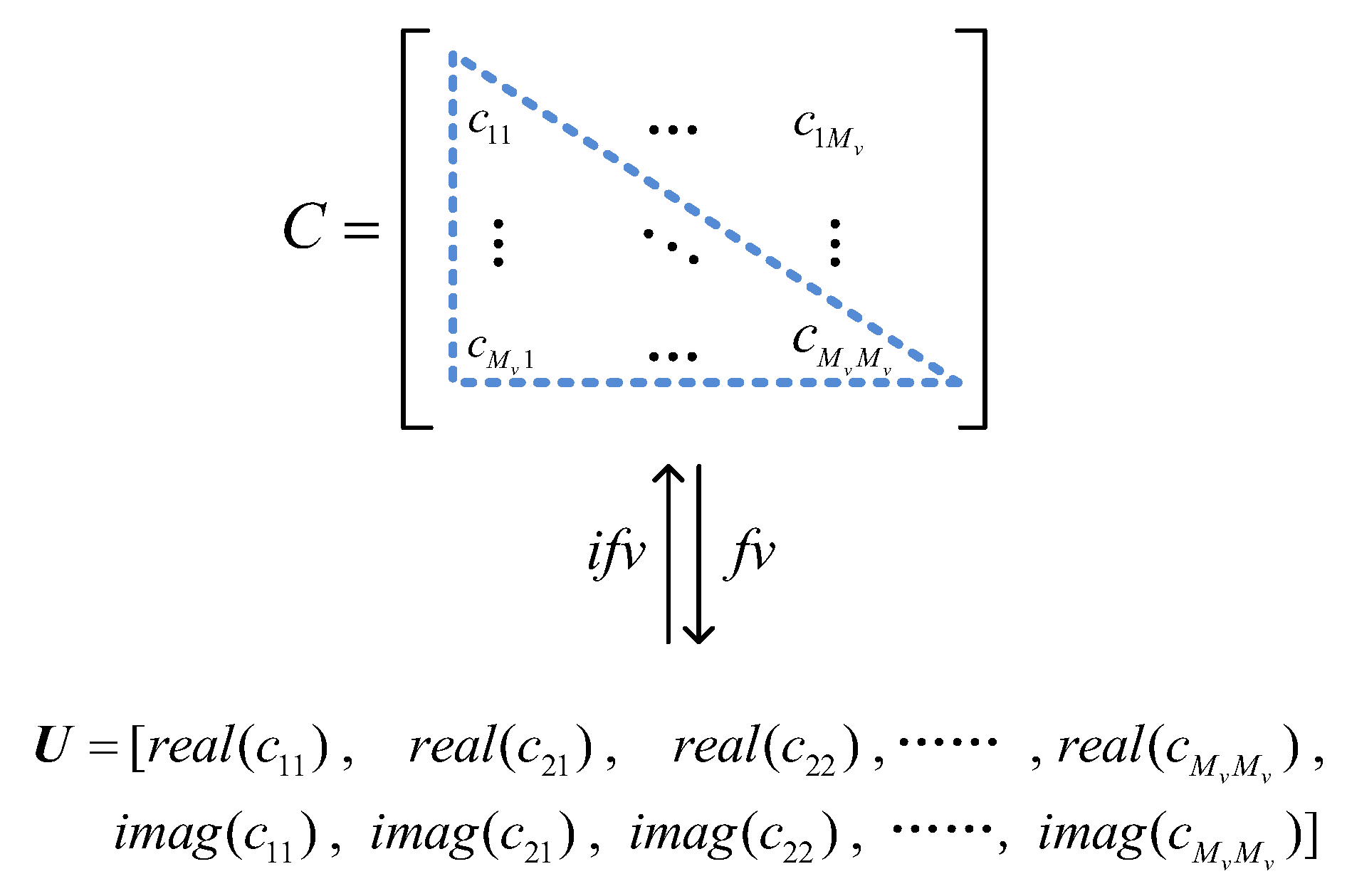
3.1. Data Preprocessing

Through data preprocessing, the M-element linear array data is transformed into vector form, and the input data suitable for the DIAE algorithm can be generated. Generally, wideband signals can be divided into multiple narrowband processes. The sample covariance matrix ${\tilde{\mathit{R}}}_x$ of each narrowband can be approximated by the frequency cross-spectral matrix $\tilde{\mathit{C}}(\omega )$,

$$\tilde{\mathit{C}}(\omega )=\frac{1}{N}{\displaystyle \sum _{n=1}^N\mathit{X}(\omega ){\mathit{X}}^{\mathrm{H}}(\omega )},$$

(14)

• $\omega$: the center frequency of the narrowband;
• $\mathit{X}(\omega )$: the Fourier transform of received array signal $\mathit{X}(t)$.

$$\tilde{\mathit{C}}\left(\omega \right)=\left[\begin{array}{cccc}{c}_{11}(\omega )& c_{12}(\omega )& \cdots & c_{1M_v}(\omega )\\ c_{21}(\omega )& c_{22}(\omega )& \cdots & c_{2M_v}(\omega )\\ ⋮& ⋮& \ddots & ⋮\\ c_{M_{v}1}(\omega )& c_{M_{v}2}(\omega )& \cdots & c_{M_v{M}_v}(\omega )\end{array}\right],$$

(15)

• $\tilde{\mathit{C}}(\omega )\in {\mathbb{C}}^{M_v\times M_v},M_v=3M.$

$\tilde{\mathit{C}}(\omega )$ is a Hermitian matrix that retrieves both the power and azimuth information of the received signal in a narrow band centered around $\omega$, and every element $c_{mn}(\omega )$ in $\tilde{\mathit{C}}(\omega )$ is the frequency domain covariance of $m$th and $n$th channels within the narrow band. The lower triangular and diagonal elements contain all information of $\tilde{\mathit{C}}(\omega )$, and Figure 2 illustrates how we obtain feature vector $\mathit{U}$ from $\tilde{\mathit{C}}(\omega )$. The real part of the lower triangular and diagonal elements of $\tilde{\mathit{C}}(\omega )$ comprise ${\mathit{U}}_{real}\in {ℝ}^{(M_v+1)M_v/2}$, and the imaginary parts comprise ${\mathit{U}}_{imag}\in {ℝ}^{(M_v+1)M_v/2}$. The feature vector $\mathit{U}={[{\mathit{U}}_{real}{}^{\mathrm{T}},{\mathit{U}}_{imag}{}^{\mathrm{T}}]}^{\mathrm{T}}$. The transformation above is defined as $\mathit{U}=fv[\tilde{\mathit{C}}(\omega )]$ and its inverse operator as $\tilde{\mathit{C}}\left(\omega \right)=ifv [\mathit{U}]$, which can map $\mathit{U}$ back to the matrix $\tilde{\mathit{C}}\left(\omega \right)\in {ℂ}^{M_v\times M_v}$.

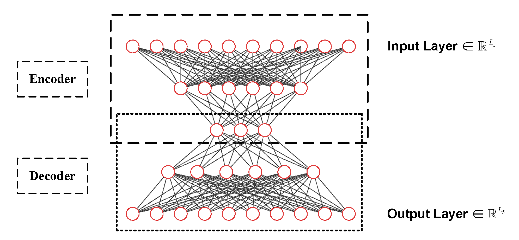
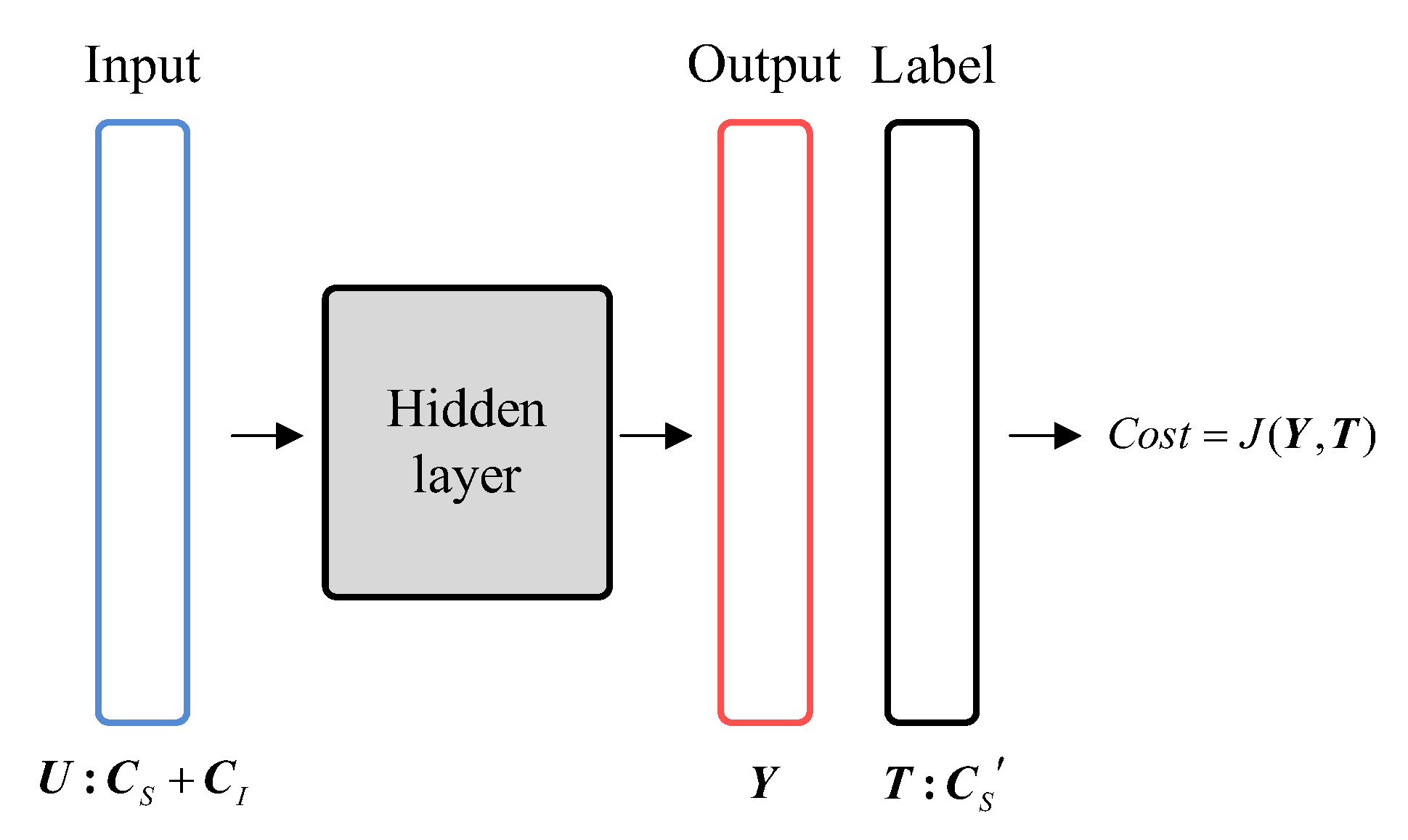
3.2. DIAE Principle

As depicted in Figure 3, the proposed DIAE algorithm has the same network structure as the traditional autoencoder, which is composed of an encoder and decoder in series. The encoder consists of an input layer and two hidden layers, each of which has $L_1$, $L_2$, and $L_3$ neurons. The decoder consists of hidden layers and an output layer, each of which has $L_3$, $L_4$, and $L_5$ neurons. The output layer of the encoder serves as the input layer of the decoder.

Equations (16) and (17) express how two adjacent layers of neurons are fully connected.

$${\mathcal{z}}^l=w^l{\mathit{a}}^{l-1}+{\mathit{b}}^l, l=2,\cdots ,5,$$

(16)

$${\mathit{a}}^l=\sigma [{\mathcal{z}}^l].$$

(17)

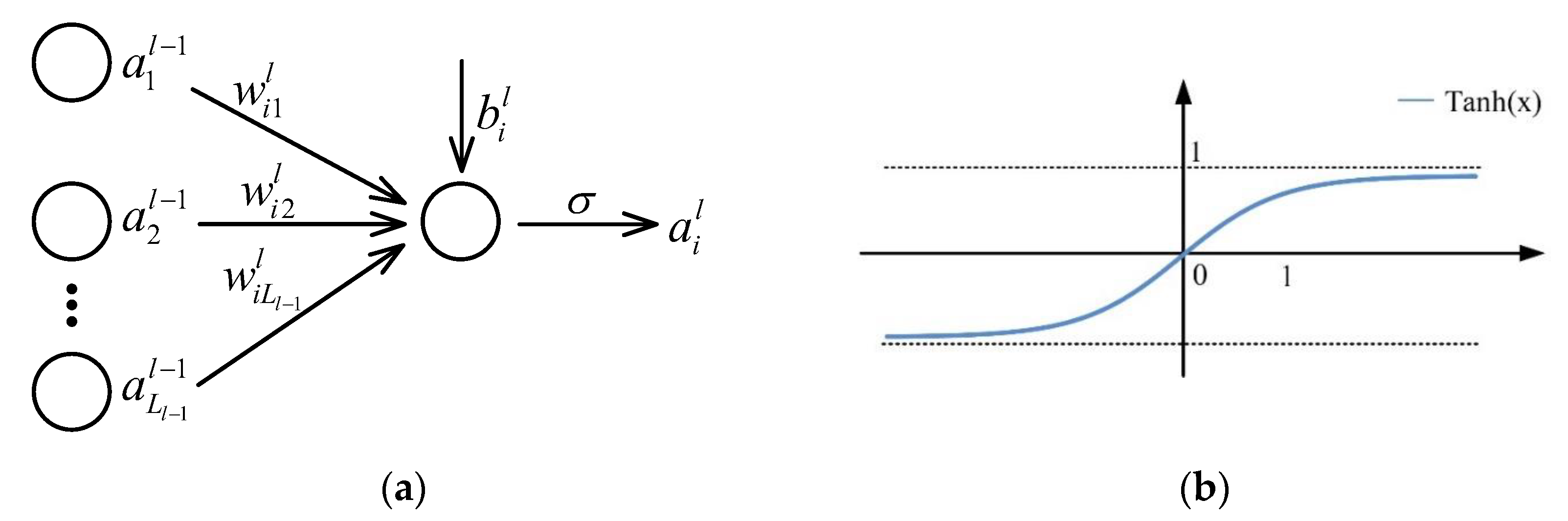
• ${\mathit{a}}^l$: ${\mathit{a}}^l={[a_1^l,a_2^l, \dots ,a_{L_l}^l]}^T$ is the output of the lth layer;
• $w^l$: the weight matrix connecting lth layer and $l-1$th layer, $w^l\in {ℝ}^{L_l\times L_{l-1}}$;
• ${\mathit{b}}^l$: ${\mathit{b}}^l={[b_1^l,b_2^l, \dots ,b_{L_l}^l]}^T$ is the bias of lth layer;
• $\sigma$: activation function.

Figure 4a shows the operation associated with the single neuron $a_i^l$ and Figure 4b illustrates the Tanh activation function employed in DIAE denoted by

$$\sigma =\mathrm{Tan}\mathrm{h}(z)=\frac{e^z-e^{-z}}{e^z+e^{-z}}.$$

(18)

Tanh is ideal for training neural networks as it balances both training speed and stability, and, more importantly, it can keep the neuron activation values within the range of (−1,1). This makes it easier for the output to fit the real and imaginary parts of the SCM.

The conventional autoencoder model takes the reconstruction error of the input value as the loss function, and the learning process can be described as minimizing the loss function,

$$\underset{f,g}{\arg \min }J(\mathit{Y},\mathit{U})=\underset{f,g}{\arg \min }J\{g[f(\mathit{U})],\mathit{U}\},$$

(19)

where $\mathit{H}=f\left(\mathit{U}\right)$ and $\mathit{Y}=g\left(\mathit{H}\right)$, representing the encoder and decoder, respectively. $J$ is the cost function denoting the difference between the output $\mathit{Y}$ and the input $\mathit{U}$. The dimension of the output layer of the encoder is smaller than that of the input layer, forcing the autoencoder algorithm to learn the most prominent features in the feature distribution.

When the UUV is detecting the target, the target of interest usually has a varying azimuth and radiated noise power, while the platform interference received by the flank array is short-term and stationary. The DIAE algorithm has been designed for suppressing the platform interference from the received array data. Figure 5 and the following explanation illustrate the innovation and technical details of DIAE.

• The DIAE model takes the preprocessed SCMs as input $\mathit{U}$, reduces the feature dimension through the encoder, and the output $\mathit{Y}$ is restored to the original dimension by the decoder. Through the $ifv$ transformation introduced in Section 2, the output $\mathit{Y}$ can transform into SCM without interference;
• A dominant label $\mathit{T}$ is designed to make DIAE an interference suppression algorithm. Through carefully designed labels, the DIAE model can learn the most prominent features in SCM and suppress the feature components of interference. Every input $\mathit{U}$ is preprocessed from SCM which is composed of the far-field target feature ${\mathit{C}}_S$ and the near-field interference feature ${\mathit{C}}_I$; The corresponding label $\mathit{T}$ is preprocessed from SCM which is composed of the far-field target feature ${\mathit{C}}_S{}^{\prime }$. Ideally, ${\mathit{C}}_S{}^{\prime }$ is equal to ${\mathit{C}}_S$;
• Root mean square error (RMSE) is set as the cost function of the DIAE algorithm to minimize input and output errors.

For practical application, we propose a theoretically optimal way to collect and construct training samples, making ${\mathit{C}}_S{}^{\prime }$ an approximation of ${\mathit{C}}_S$. As we know, the propeller noise is considered as the major near-field interference of the UUV in many cases. By alternating the rotation and stoppage of the propeller within a short time period, the propeller interference occurs intermittently. Meanwhile, the far-field signal features can be considered relatively stable during these short intervals of propeller state-switching. Therefore, it is possible to obtain multiple pairs of $\{\mathit{U},\mathit{T}\}$ during these intervals. However, this method for collecting training samples is time-consuming and laborious, and we put forward an easier and cheaper way in our lake experiment in Section 5.

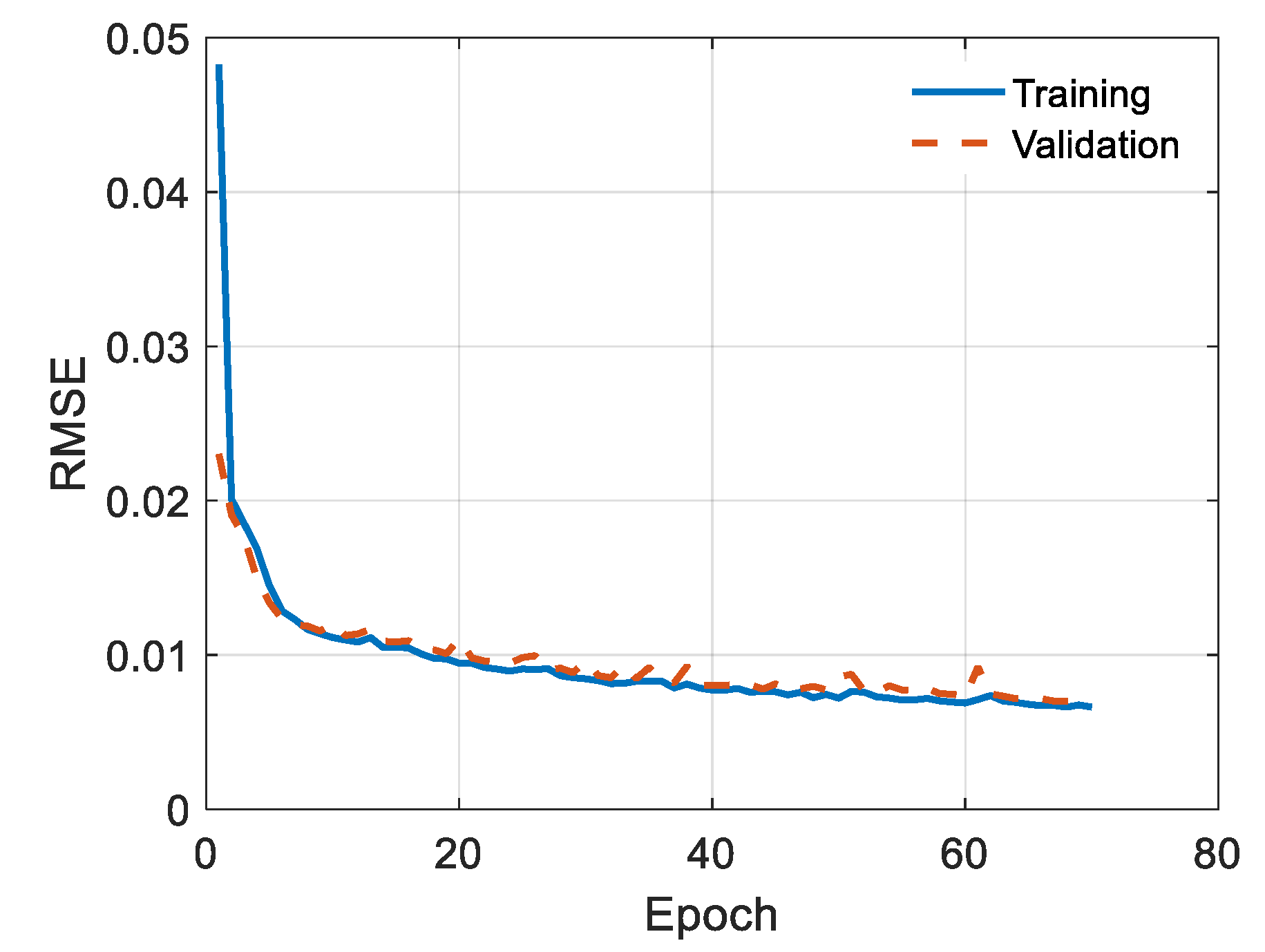
3.3. DIAE Training

DIAE is trained with the gradient descent method, and the network parameters are updated by back propagation [26]. The training aim can be expressed as

$$\begin{array}{cc}\underset{\mathit{W},\mathit{B}}{\arg \min }& J=\frac{1}{Z}{\displaystyle \sum _1^Z{‖{\mathit{Y}}_i-{\mathit{T}}_i‖}_2},\hfill \\ & \mathit{W}=\left\{{\mathit{w}}^l|l=2,3,4,5\right\},\hfill \\ & \mathit{B}=\left\{{\mathit{b}}^l|l=2,3,4,5\right\}\hfill \end{array}$$

(20)

• $J$: the cost function averaged over $Z$ training samples;
• ${‖ · ‖}_2$: 2-norm operation of vectors.

The training process continues until training parameters $\mathit{W}$ and $\mathit{B}$ approximate the optimal value. The minibatch strategy [27] is followed with a batch size of 64, and the Adam gradient optimization algorithm [28] is chosen to accelerate gradient descent with a learning rate of 0.001 and weight decay of 0.05. To prevent the model from overfitting, a certain proportion of the training set samples are set aside as validation to evaluate the DIAE training results. In general, if the cost curve along with the training epoch of the training set is similar to that of the verification set, it implies that the learned features are not limited to the training set alone, suggesting the absence of overfitting. After training, gradients of $\mathit{W}$, $\mathit{B}$ are no longer updated, and the model can be used for suppressing interference.

4. Simulation and Analyses

This section carries out simulations to show the predominance of the proposed method over existing near-field interference suppression methods. The simulations are implemented using the PyTorch [29] framework, which can provide full support for neuron network building and training. Matrix Filter (MF) and focused inverse beamforming (FIBF) are chosen as comparison algorithms. The simulation parameters are as follows. Unless noted otherwise, the parameters remain constant throughout this section.

A nine-element uniform vector linear array is employed in the simulations with a spacing interval $d=0.33 \mathrm{m}$. The interferences consist of multiple independent near-field point sources, and the target of interest is a far-field signal. For narrowband processing, the central frequency is set at $f_0$ = 2267 Hz, corresponding to half a wavelength, with a bandwidth of $B_0$ = 180 Hz. The noise at each sensor is additive Gaussian noise. The signal-to-noise ratio (SNR) and interference-to-noise ratio (INR) are defined as the narrowband power ratios at the reference sensor. The array receiving data is generated by the above-mentioned parameters with a time length of $T_0$ = 0.4 s, and can be transformed to a dataset sample by data preprocessing. To enhance the dataset’s diversity, the receiving data is generated with randomized interference and target parameters. The INR, $r_N$, and ${\theta }_N$ parameters follow a uniform distribution, with specified lower and upper values for each parameter outlined in

Table 2. Parameters of simulation array receiving data.

Interferences	INR	$\mathbf{Position} ({\mathit{r}}_{\mathit{N}},{\mathit{\theta }}_{\mathit{N}})$
	15 ± 1 dB	(300 ± 2°, 1.2 ± 0.1 m)
		(315 ± 2°, 0.6 ± 0.1 m)
Target	SNR	Azimuth ${\mathit{\theta }}_{\mathit{F}}$
	[−5, 10] dB	[30°, 150°]∪[240°, 290°]

. The SNR and ${\theta }_F$ parameters are random sampling from the given interval. The interferences consist of two near-field point sources with equal power, and the interference-to-noise ratio (INR) is determined based on the total interference energy. A total of $N_{all}$ = 8000 dataset samples are generated. Among them, the proportion of training set, verification set, and test set is 60%, 20%, and 20%.

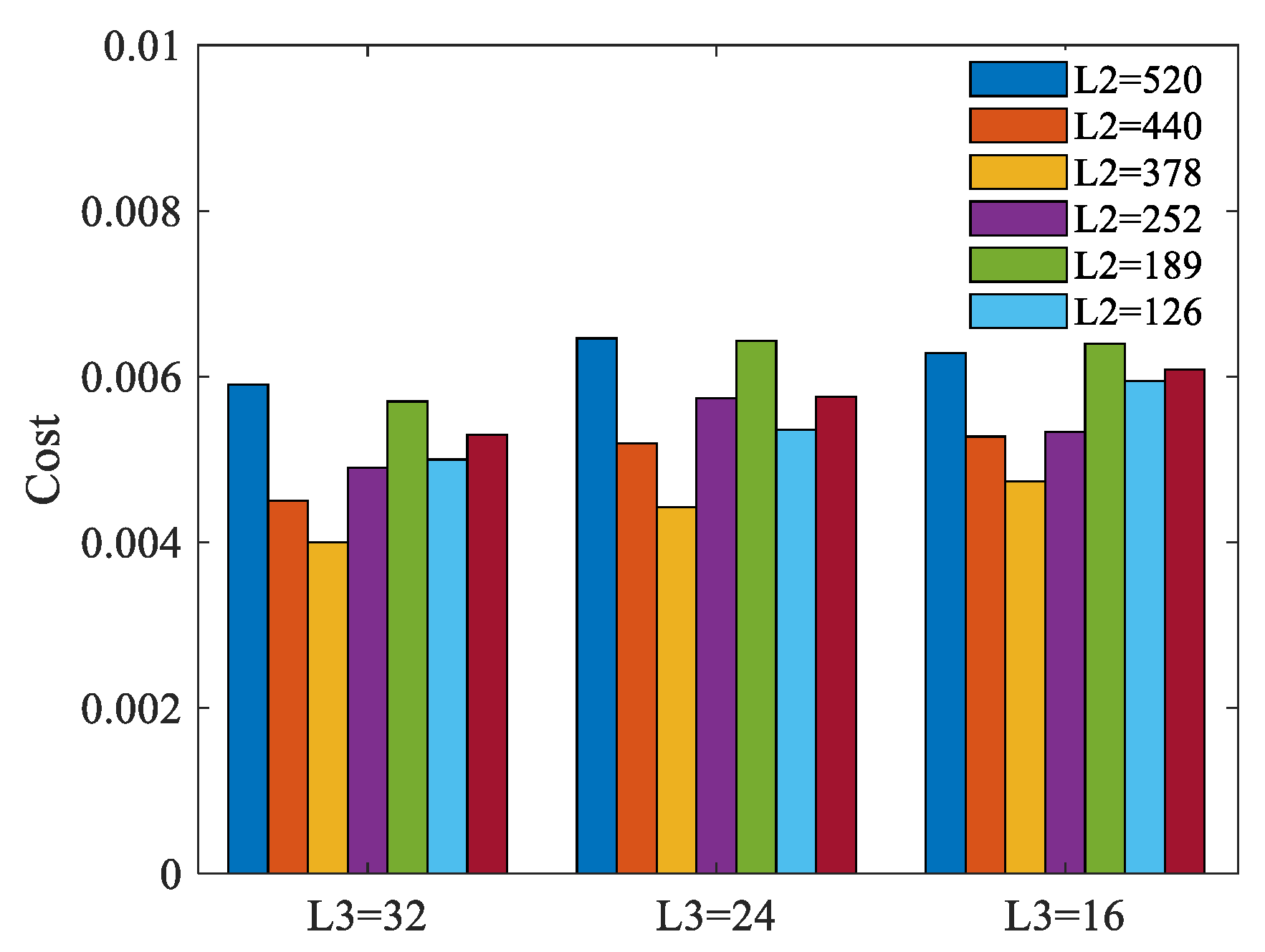
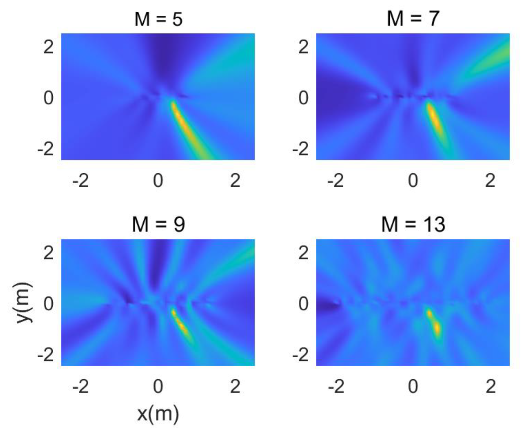
4.1. Parameter Optimization

In order to optimize the performance of the DIAE model, grid search is employed in the numbers of neurons in hidden layers:$L_2$, $L_3$. The 4-fold cross-validation technique is utilized to evaluate the generalization ability of the DIAE, and the total cost function of the trained model is denoted as $J{\{\mathit{Y},\mathit{T}\}}_{4-fold}$,

$$J{\{\mathit{Y},\mathit{T}\}}_{4-fold}=\frac{1}{4}{\displaystyle \sum _1^4{\displaystyle \sum _{i=1}^{N_{test}}{‖{\mathit{Y}}_i-{\mathit{T}}_i‖}_2}}.$$

(21)

Figure 6 indicates $L_2=378$, $L_3=32$ to be optimal and, based on this pair of parameters, the subsequent simulation model is constructed; more specific parameters of DIAE are listed in

Table 3. Parameters of DIAE model.

Layers	Hyperparameters	Total Parameters
Encoder input	$L_1=756$, FC 1	0
Hidden layer	$L_2=378$, FC, Tanh	2628
Hidden layer	$L_3=32$, FC, Tanh	592
Hidden layer	$L_4=378$, FC Tanh	592
Decoder output	$L_5=756$, FC, Tanh	2628

¹ FC is short for fully connected. Total parameters denote the quantities of training parameters.

.

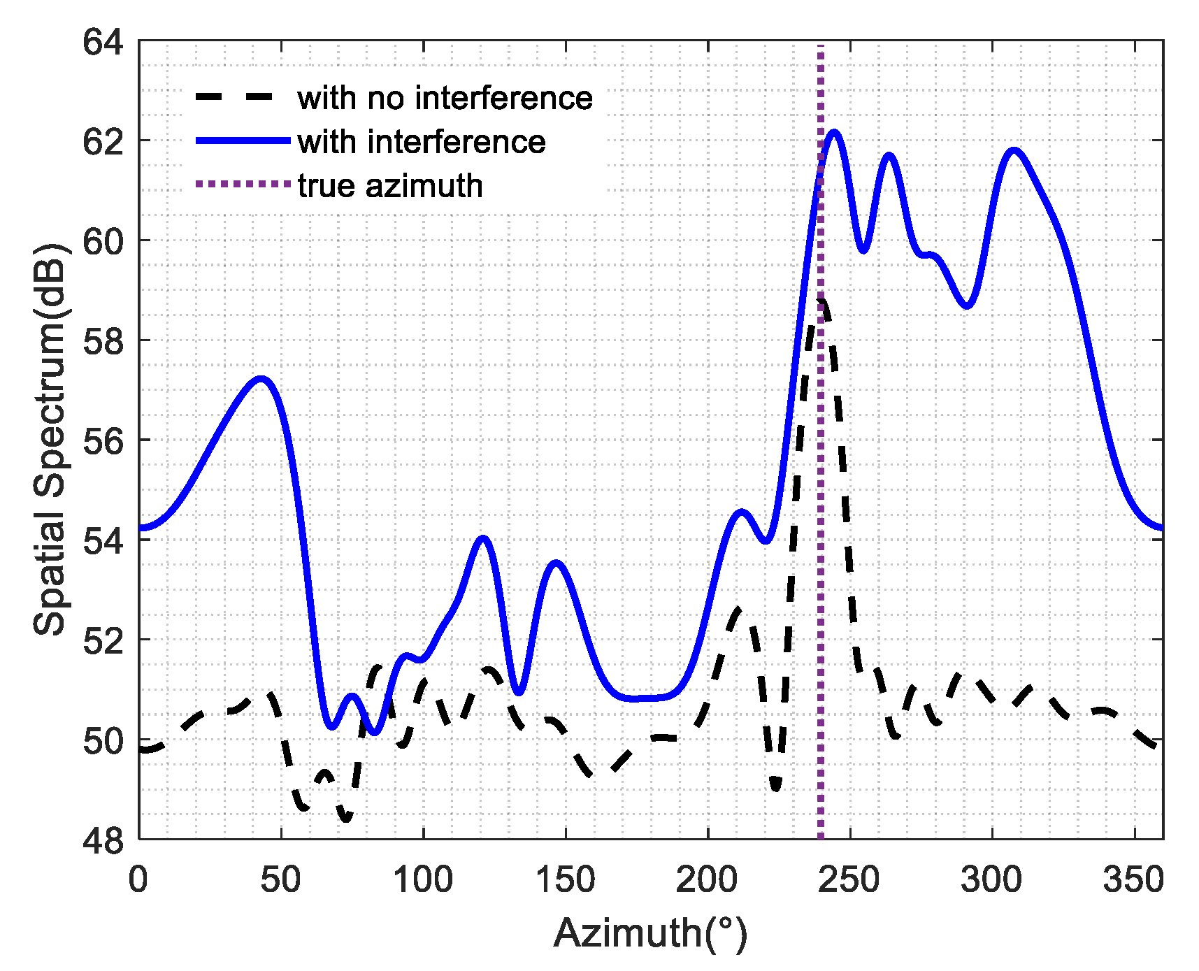
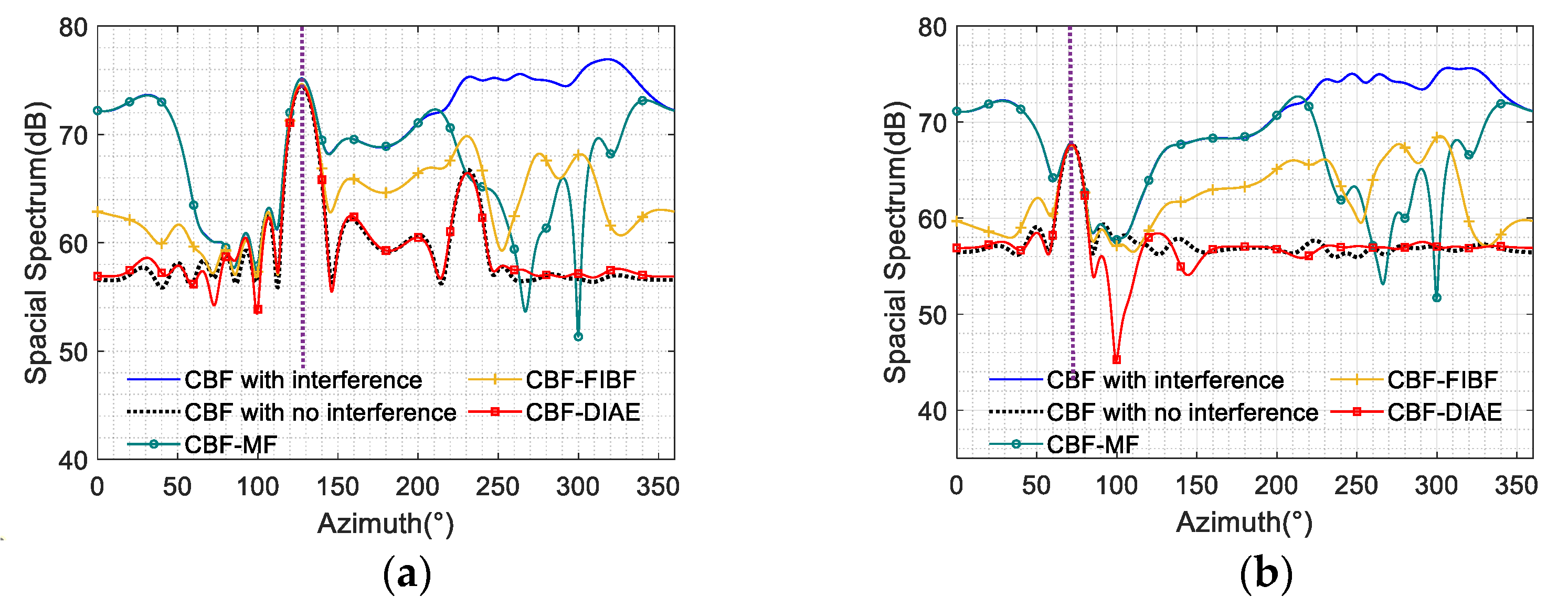
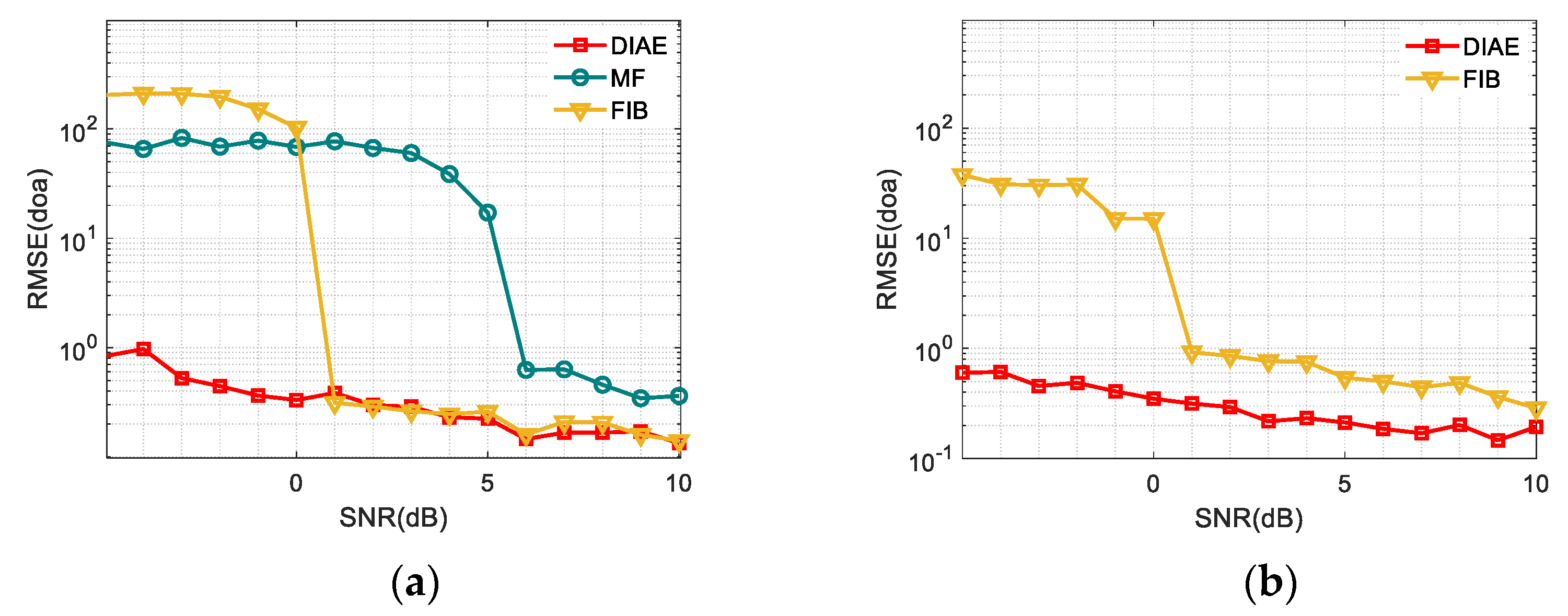
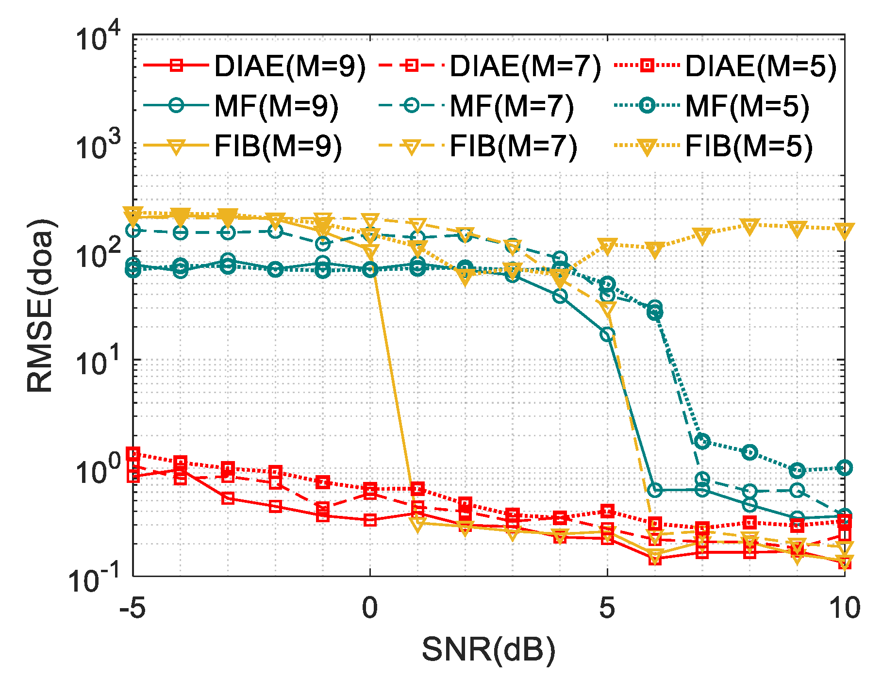
4.2. Performance Analysis

DOA based on Conventional Beamforming, referred to as CBF, can estimate source azimuth by assuming plane wave propagation [30]. CBF calculates a spatial spectrum as its output, which can be mathematically expressed as follows:

$${\delta }^2{}_{\mathrm{CBF}}(\theta )=a_F{(\theta )}^{\mathrm{H}}{\mathit{C}}_{\omega }{a}_F(\theta ).$$

(22)

• $a_F(\theta )$: steeling vector of plane wave impinging from azimuth ${\theta }^{\circ }$.

Since the amplitude of the spectrum represents the actual power spectrum, we employ the CBF spatial spectrum to analyze the performance of interference suppression. For our method, ${\mathit{C}}_{\omega }$ derives from the transform ${\mathit{C}}_{\omega }=ifv[\mathit{Y}]$, where $\mathit{Y}$ is the output of DIAE.

Figure 7 shows the impact of near-field interference on the spatial spectrum. The near-field interference is located at $\left({\rho }_N,{\theta }_N\right)=\left(1.2\mathrm{m}, 300°\right)$ with INR = 5 dB, and the far-field target comes from $\theta ={240}^{\circ }$ with SNR = −5 dB. The presence of near-field interference leads to a strong power leakage in the target azimuth and, as a result, the spatial spectrum peak of the target gets submerged. In addition to this, Figure 7 implies that the energy of the near-field interference leaks to a large range of the far-field azimuth under the specified simulation conditions.

In the subsequent simulation, we assess the performance of the proposed algorithm by conducting comparative analyses. We tried to achieve the best performance of the comparison algorithms in the simulation.

The Matrix Filter algorithm (MF) assumes that the signal and interference exist in separate azimuth sectors and requires knowledge of the interference’s approximate position. Equation (23) describes the solution of the filter matrix $G$ (for more details, see Liang et al. [9]). The solution can be transformed into a second-order cone programming (SOCP) and solved with CVX toolbox.

$$\begin{array}{c}\min {\max }_{j=1,\cdots ,P}‖G^{H}a({\theta }_j)-a({\theta }_j)‖,{\theta }_j\in {\mathrm{\Theta }}_P\\ \mathrm{s}.\mathrm{t}. ‖G^{H}a(r_i,{\theta }_i)‖\le {\xi }_0, (r_i,{\theta }_i)\in {\mathrm{\Theta }}_S,i=1,\cdots ,S\\ {‖G^H‖}_F\le {\mathrm{\Delta }}_0\end{array}$$

(23)

• ${\mathrm{\Theta }}_S$: the stopband in the near field;
• ${\mathrm{\Theta }}_P$: the passband in the far field;
• ${\xi }_0$: the attenuation in the suppressed area;
• ${‖ · ‖}_F$: Frobenius norm operation of matrices;
• ${\mathrm{\Delta }}_0$: the white noise limitation.

In the simulation, we assume that the interference area is known, as Table 2 denotes, and set the parameters as follows:

$$\begin{array}{cc}{\mathrm{\Theta }}_S=& \{(x,y)|x=[0.3:0.1:0.8],y=[-1.3:0.1:-0.7]\}\hfill \\ {\mathrm{\Theta }}_P=& [0^{\circ }:{10}^{\circ }:{210}^{\circ }]\hfill \\ {\xi }_0=& 0.1, {\mathrm{\Delta }}_0=4.0\hfill \end{array}$$

(24)

${\mathrm{\Theta }}_S$ is a set of spatial location coordinates that cover the position of the interferences. ${\mathrm{\Theta }}_P$ is a set of angles that cover the far-field passband. The value of ${\xi }_0$ and ${\mathrm{\Delta }}_0$ are set with optimal after several attempts.

The FIBF algorithm does not need prior information on interference, but its performance is closely related to the accuracy of interference source location estimation. In order to ensure the location accuracy, a sufficient array aperture is needed. Generally, multiple iterations are necessary for better results [6]. In our simulation, the number of iterations is set equal to the number of near-field sources, as we confirm it to be appropriate through multiple attempts.

The DIAE algorithm is trained using a simulation dataset constructed with parameters outlined in Table 2. Dual interference sources are at $(r_1,{\theta }_1)=(1.2 \mathrm{m}, 300°)$, $(r_2,{\theta }_2)=(0.6 \mathrm{m}, 315°)$, respectively (Due to the way the dataset is constructed, there is a deviation in the real interference position). Figure 8 depicts the outcomes of interference suppression algorithms under two distinct SNR levels. By comparing the azimuth spectrum in the presence and absence of interference, we observe that the interference energy leaks into a large range of far-field azimuth, which makes it a big challenge for detecting the target even when quite far away from the interference sector. The DIAE algorithm demonstrates its superior effectiveness in completely suppressing interference, as evidenced by the spatial spectrum estimation outcomes. The FIBF algorithm suppresses partial interference energy and highlights the spatial spectrum peak of the target. However, in cases where the SNR drops to −2 dB (see Figure 8b), the target’s spatial spectrum peak can fall below that of the interference spatial spectrum peak, posing challenges in target detection. The MF algorithm suppresses the interference energy of the azimuth of the interference better than the FIBF algorithm, but lacks the ability to suppress the energy leaked to the passband azimuth.

In the following simulation, we analyze how SNRs impact algorithm performance by counting the root mean square error (RMSE) of the first spectral peak estimation. The azimuth relationship between the target and the interference is taken into account, and the analysis is conducted separately for two cases: when the target angle is away from the interference angle, and when the target angle is close to the interference angle.

Figure 9a presents the accuracy of spectral peak estimation when the target azimuth falls in the range of [30°, 150°]. The DIAE algorithm performed well, producing low RMSE values for spectral peak estimation across different SNRs. The FIBF algorithm has limited interference suppression ability due to the estimation accuracy of the reference interference signal. In the case of low SNRs, the leaked interference energy at a certain azimuth is higher than the target spectrum peak, resulting in an inaccurate estimation of the target spectrum peak position. The MF algorithm has less ability to suppress the energy leaking into the target azimuth than FIBF, so it has the worst performance in low SNRs.

Figure 9b presents the accuracy of spectral peak estimation when the target azimuth falls in the range of [240°, 290°]. Since the MF algorithm cannot be applied to the case where the target azimuth is close to the interference azimuth, we omit the statistics on the performance of the MF algorithm. Results show that the performance of the DIAE algorithm is still better than that of the FIBF algorithm in this situation.

Next, we analyze how the number of sensors impacts algorithm performance. $M=$ 5, 7, 9 are set as the number of sensors. The corresponding parameter changes in each algorithm are presented in

Table 4. Algorithm parameters for various numbers of sensors.

M	DIAE	MF	FIBF
5	$L_m=[240,72,16],m=1,2,3$	$\xi =0.1,\mathrm{\Delta }=2.0$	-
7	$L_m=[420,180,24],m=1,2,3$	$\xi =0.1,\mathrm{\Delta }=3.5$	-
9	$L_m=[756,378,32],m=1,2,3$	$\xi =0.1,\mathrm{\Delta }=4.0$	-

. The FIBF algorithm parameters keep constant.

Figure 10 presents the variation of spectral peak estimation accuracy with the number of sensors. The RMSEs are obtained from the samples in the azimuth range of [30°, 150°]. The result shows that the DIAE algorithm performs robust interference suppression capabilities and is less affected by changes in the number of sensors. Even with a small number of sensors, the DIAE algorithm effectively suppresses interference and accurately estimates the signal spectrum peak. In contrast, the performance of the FIBF algorithm is greatly affected by the number of sensors. FIBF exhibits proficient performance when the number of sensors is considerable, yet demonstrates a discernible decline in performance as the number of sensors decreases. As shown in the illustration, the FIBF algorithm performs poorly across all tested SNRs when the number of sensors equals 5. The performance of the MF algorithm also depends on the number of sensors but, when the number of elements degrades, its performance degradation is less than that of the FIBF algorithm.

Figure 11 provides a visual representation of why the effectiveness of the FIBF algorithm is heavily influenced by the number of sensors. It presents the results of focused beamforming when dealing with near-field interference under varying numbers of sensors. The findings reveal that the decrease in the number of sensors leads to a wider near-field focusing peak. As a consequence, the focusing peaks of the interference sources merge, making it challenging to accurately estimate their positions and impeding the performance of the FIBF algorithm. In contrast, our DIAE algorithm inherently avoids constructing a propagation model of near-field interference and exhibits minimal performance degradation in scenarios with fewer sensors.

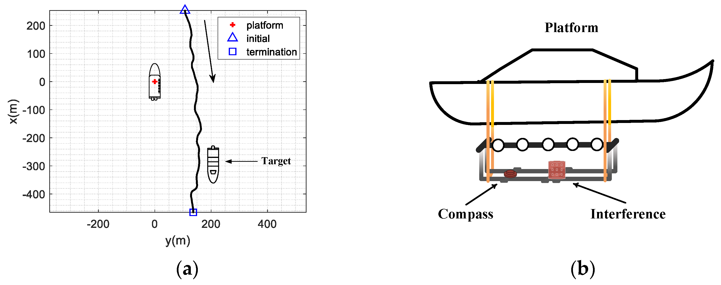
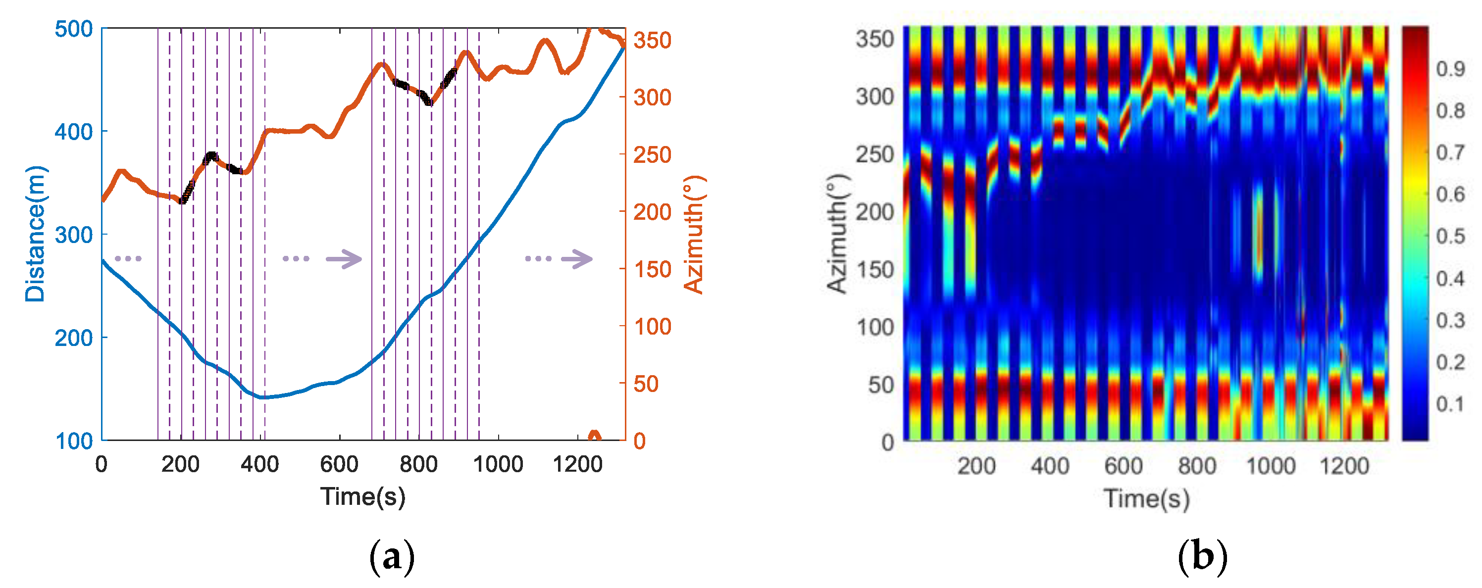
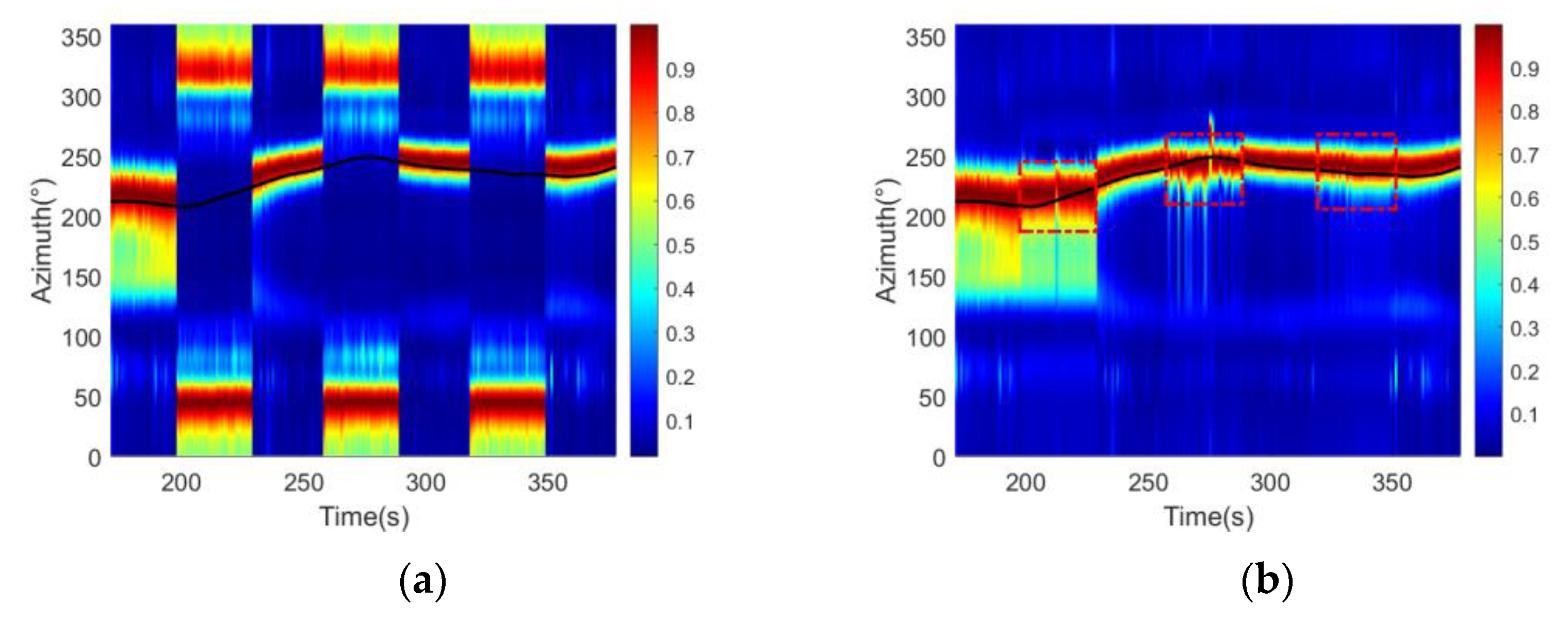
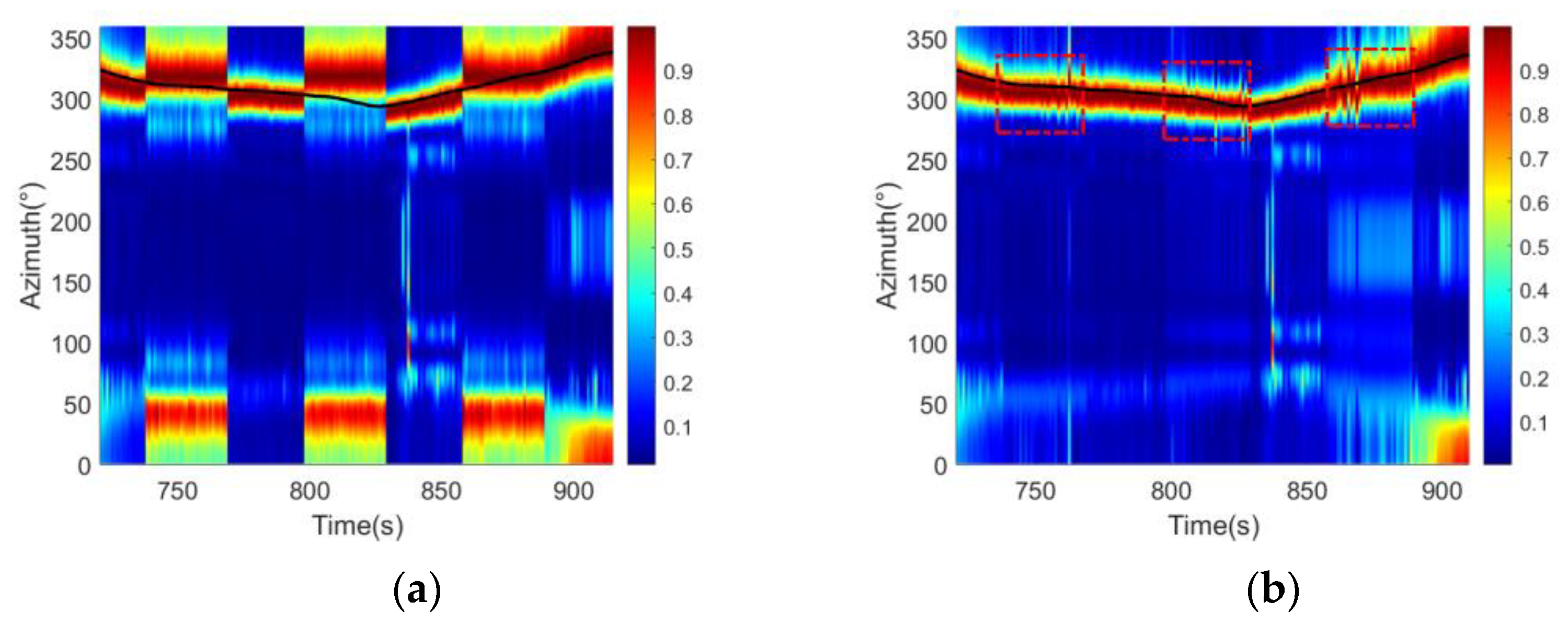
5. Lake Experiment

The experimental data is from the technical verification experiment for interference suppression conducted in Songhua Lake in Jilin Province, China in October 2022. Figure 12 shows the sketch of this experiment. The experiment involved a platform anchored in the water, designed to simulate a UUV. A five-element uniform vector linear array was suspended at a depth of 3m. The array direction was calibrated using a compass equipped on the array shelf. A fixed interference source was placed in the near-field region of the array to simulate near-field interference caused by the UUV. For dataset construction purposes, the interference source was configured to transmit for 30 s, with intervals of 60 s. During the experiment, a target ship equipped with a GPS was nearly the only visible ship within the observation range.

Figure 13a shows the distance and azimuth between the platform and targets solved by a joint GPS and compass fixed on the array. The vertical lines, spaced 30 s apart, indicate the start or stop times of the interference source. Figure 13b presents the BTR results obtained by conventional beamforming (CBF) algorithm. As shown in the graph, when interference is present in 30 s, the spatial spectrum of the interference is concentrated around 40° and 320°, which is obviously higher than that of the target, so that the target’s azimuth cannot be estimated accurately. Conversely, the target’s azimuth can be accurately estimated when there is no interference.

The construction process of the dataset is as follows: All 1320 s data are segmented by a time window of $\mathrm{\Delta }T=0.4 s$ without overlapping. The preprocessing result of each segment is ${\mathit{U}}_i, i=1,2,\dots ,3300$. The test set is composed of ${\mathit{U}}_i$s which come from time period marked with black lines in Figure 13a, with a total of 450 samples. For facilitating the follow-up analysis, we divided them into two distinct time periods: ${\mathrm{\Gamma }}_1$,${\mathrm{\Gamma }}_2$.

• ${\mathrm{\Gamma }}_1$: [201 s, 230 s]∪[261 s, 290 s]∪[321 s, 350 s];
• ${\mathrm{\Gamma }}_2$: [741 s, 770 s]∪[801 s, 830 s]∪[861 s, 890 s].

A simple method is devised to generate the training set samples, resulting in a total of 8202 samples. Each {${\mathit{U}}_i$,${\mathit{U}}_j$} in the training set satisfies the following conditions: (1) ${\mathit{U}}_i$ derives from interference time period except the test set period. (2) ${\mathit{U}}_j$ derives from a non-interference time period. (3) ${\mathit{U}}_i$, ${\mathit{U}}_j$ own the same true value of the target azimuth, which is the joint solution result of GPS and compass.

DIAE is trained with the hyper-parameters and dataset shown in

Table 5. Parameters for lake data processing.

DIAE
Hyper-parameters	$L_m=[240,72,16,72,240], m=1,\dots ,5$. FC, Tanh
Dataset
Total	8202
Division	Train:Validation:Test = 6202:1550:450

. The training strategies remain unchanged as mentioned in Section 3.3. Figure 14 shows the training process. The training process stops at the 70th epoch. With the increase in training epochs, the loss of the validation set and the training set exhibit similar curves, signifying that the training is not experiencing over-fitting. The duration of each epoch is 0.58 s on average with operation accelerated by an Nvidia RTX3060. For the test process, the duration for forward propagation takes less than 0.01 s in a batch of 225 samples. This proves that DIAE is an efficient algorithm capable of real-time interference suppression.

Figure 15 shows the bearing time record from 172 s to 378 s of the experiment. Black lines represent the true azimuth trajectory. Figure 15a shows the origin BTR of the experiment. Within the time period, test samples derived from time duration ${\mathrm{\Gamma }}_1$ are applied into the trained DIAE model. In Figure 15b, we replace the origin BTR in the corresponding time period with DIAE outcomes, which are highlighted by the red dotted box. The DIAE algorithm has been observed to be highly efficient in eliminating interference components within the received signal. After the suppression of interference, the corresponding time period data is viable for the estimation of the target azimuth. The azimuth estimation displays a similar trace as the true azimuth trajectory.

Figure 16 shows the DIAE performance in another case, in which the target azimuth is close to the interference. Figure 16a is the origin BTR of the experiment from 718 s to 912 s, while the interferences exist in time period ${\mathrm{\Gamma }}_2$. Figure 16b shows that DIAE performs well in suppressing interferences when the target azimuth is close to the interference.

Mean absolute error (MAE) is used to evaluate the accuracy of azimuth estimation after interference suppression, which is defined as

$$\mathrm{MAE}=\frac{1}{n}{\displaystyle \sum _{i=1}^n\left|\theta -\widehat{\theta }\right|}.$$

(25)

• $\widehat{\theta }$: estimation of azimuth based on spectrum peak;
• $\theta$: the true value of azimuth.

The MAE results under two scenarios are counted separately and shown in

Table 6. MAE results of DOA estimation.

MAE Results (°)
	172 s to 378 s (Figure 15)	718 s to 912 s (Figure 16)
Interference	187.7	10.1
Interference suppression	7.3	7.4
No Interference	6.2	5.4

. MAEs under three situations shows the performance of DIAE algorithm.

Unexpectedly, the MF algorithm and FIBF algorithm display low capability in suppressing the near-field interference in the lake experiment. However, the simulation results have provided valuable insights into this phenomenon. It has been noted that both comparison algorithms exhibit a significant reduction in performance when the number of sensors is limited. Additionally, accurately estimating the true steering vectors of interference in the lake experiment remains a considerable challenge and further limits the effectiveness of both algorithms. In the lake experiment, the received signal does not show an apparent spectrum peak in the near-field acoustics image. Our proposed DIAE algorithm, on the other hand, is not restricted by such limitations and can be effectively applied to suppress near-field interference in experimental data.

6. Conclusions

This paper proposes an improved autoencoder algorithm for suppressing self-interference of unmanned underwater vehicles to make up for the drawbacks of existing methods in terms of interference estimation and cancellation. The proposed DIAE algorithm realizes the extraction and cancellation of platform self-interference by compressing and reconstructing the array signal features. Since it does not require the estimation of the interference source locations and the steering vectors of the interference signal, our method avoids the performance loss caused by the mismatch of the interference model. Simulations prove that the proposed method outperforms the compared methods when working with limited sensors and low signal-to-noise ratios. Moreover, the lake experiment confirms the effectiveness of our method in challenging underwater environments, demonstrating its superiority over existing methods.

References

- Arrabito, G.R.; Cooke, B.E.; McFadden, S.M. Recommendations for Enhancing the Role of the Auditory Modality for Processing Sonar Data. Appl. Acoust. 2005, 66, 986–1005. [Google Scholar] [CrossRef]
- Gorriz, J.M.; Ramirez, J.; Cruces-Alvarez, S.; Puntonet, C.G.; Lang, E.W.; Erdogmus, D. A Novel LMS Algorithm Applied to Adaptive Noise Cancellation. IEEE Signal Process. Lett. 2009, 16, 34–37. [Google Scholar] [CrossRef]
- Gao, W.; Huang, J.; Han, J. Multi-Channel Differencing Adaptive Noise Cancellation with Multi-Kernel Method. J. Syst. Eng. Electron. 2015, 26, 421–430. [Google Scholar] [CrossRef]
- Mei, J.; Sheng, X.; Zhang, Y.; Guo, L.; Jiang, M. The near field focus null-forming weight interference sound sources suppression technology of the underwater acoustic image measurement. J. Harbin Eng. Univ. 2012, 33, 653–660. [Google Scholar]
- Li, Y.; Sun, C.; Yu, H.; Wang, L. A Technique of Suppressing Towed Ship Noise. In Proceedings of the 2011 IEEE International Conference on Signal Processing, Communications and Computing (ICSPCC), Xi’an, China, 14–16 September 2011; pp. 1–4. [Google Scholar]
- Ning, J.; Li, S.; Li, Y.; Ye, Q. Adaptive cancellation of UUV self-noise based on the inverse focusing beamforming in near field. J. Appl. Acoust. 2020, 39, 527–535. [Google Scholar]
- Van Veen, B.D.; Buckley, K.M. Beamforming: A Versatile Approach to Spatial Filtering. IEEE ASSP Mag. 1988, 5, 4–24. [Google Scholar] [CrossRef]
- Zhu, Z.; Shi, W. Matrix Filter Design Using Semi-Infinite Programming with Application to DOA Estimation. IEEE Trans. Signal Process. 2000, 48, 267–271. [Google Scholar]
- Liang, G.; Zhao, W.; Fan, Z. Direction of Arrival Estimation under Near-Field Interference Using Matrix Filter. J. Comp. Acous. 2015, 23, 1540007. [Google Scholar] [CrossRef]
- Liu, K.; Liang, G. Near field focused beamforming based on matrix spatial prefiltering approach. J. Huazhong Univ. Sci. Technol. (Nat. Sci. Ed.) 2014, 42, 58–61. [Google Scholar]
- Fang, E.; Sun, C.; Gui, C. Self noise-reduction method based on spatial filtering for a vector flank array platform. J. Harbin Eng. Univ. 2020, 41, 1636–1641. [Google Scholar]
- Bianco, M.J.; Gannot, S.; Fernandez-Grande, E.; Gerstoft, P. Semi-Supervised Source Localization in Reverberant Environments with Deep Generative Modeling. IEEE Access 2021, 9, 84956–84970. [Google Scholar] [CrossRef]
- Cao, H.; Wang, W.; Su, L.; Ni, H.; Ma, L. Deep Transfer Learning for Underwater Direction of Arrival Using One Vector Sensor. J. Acoust. Soc. Am. 2021, 149, 1699–1711. [Google Scholar] [CrossRef]
- Ge, F.X.; Bai, Y.; Li, M.; Zhu, G.; Yin, J. Label Distribution-Guided Transfer Learning for Underwater Source Localization. J. Acoust. Soc. Am. 2022, 151, 4140–4149. [Google Scholar] [CrossRef] [PubMed]
- Liu, Y.; Niu, H.; Li, Z. A Multi-Task Learning Convolutional Neural Network for Source Localization in Deep Ocean. J. Acoust. Soc. Am. 2020, 148, 873–883. [Google Scholar] [CrossRef] [PubMed]
- Niu, H.; Reeves, E.; Gerstoft, P. Source Localization in an Ocean Waveguide Using Supervised Machine Learning. J. Acoust. Soc. Am. 2017, 142, 1176–1188. [Google Scholar] [CrossRef] [Green Version]
- Lefort, R.; Real, G.; Drémeau, A. Direct Regressions for Underwater Acoustic Source Localization in Fluctuating Oceans. Appl. Acoust. 2017, 116, 303–310. [Google Scholar] [CrossRef]
- Jiang, J.; Wu, Z.; Huang, M.; Xiao, Z. Detection of Underwater Acoustic Target Using Beamforming and Neural Network in Shallow Water. Appl. Acoust. 2022, 189, 108626. [Google Scholar] [CrossRef]
- Liu, Y.; Chen, H.; Wang, B. DOA Estimation Based on CNN for Underwater Acoustic Array. Appl. Acoust. 2021, 172, 107594. [Google Scholar] [CrossRef]
- Wu, L.; Liu, Z.M.; Huang, Z.T.; Wu, G. Deep Neural Network for DOA estimation with unsupervised pretraining. In Proceedings of the IEEE International Conference on Signal, Information and Data Processing, Chongqing, China, 11–13 December 2019. [Google Scholar]
- Yao, Y.; Lei, H.; He, W. Wideband DOA Estimation Based on Deep Residual Learning with Lyapunov Stability Analysis. IEEE Geosci. Remote Sens. Lett. 2022, 19, 5. [Google Scholar] [CrossRef]
- Liu, Z.M.; Zhang, C.; Yu, P.S. Direction-of-Arrival Estimation Based on Deep Neural Networks with Robustness to Array Imperfections. IEEE Trans. Antennas Propag. 2018, 66, 7315–7327. [Google Scholar] [CrossRef]
- Bianco, M.J.; Gerstoft, P.; Traer, J.; Ozanich, E. Machine Learning in Acoustics: Theory and Applications. J. Acoust. Soc. Am. 2019, 146, 3590–3628. [Google Scholar] [CrossRef] [Green Version]
- Owsley, N.L. Sonar array processing. In Array Signal Processing; Prentice-Hall, Inc.: Hoboken, NJ, USA, 1985. [Google Scholar]
- Shchuro, V.A. Vector Acoustics of the Ocean; Dalnauka: Vladivostok, Russia, 2006. [Google Scholar]
- Rumelhart, D.E.; Hinton, G.E.; Williams, R.J. Learning Representations by Back-Propagating Errors. Nature 1986, 323, 533–536. [Google Scholar] [CrossRef]
- Cotter, A.; Shamir, O.; Srebro, N.; Sridharan, K. Better Mini-Batch Algorithms via Accelerated Gradient Methods. Adv. Neural Inf. Process. Syst. 2011, 24, 1647–1655. [Google Scholar]
- Kingma, D.P.; Ba, J. Adam: A Method for Stochastic Optimization. arXiv 2014, arXiv:1412.6980. [Google Scholar]
- Paszke, A.; Gross, S.; Massa, F.; Lerer, A.; Chintala, S. PyTorch: An Imperative Style, High-Performance Deep Learning Library. In Proceedings of the 33rd Conference on Neural Information Processing Systems, Vancouver, BC, Canada, 8–14 December 2019. [Google Scholar]
- Defatta, D.J.; Lucas, J.G.; Hodgkiss, W.S. Digital Signal Processing: A System Design Approach. Append. A Conv. Beamforming 1988, 628–646. Available online: https://cir.nii.ac.jp/crid/1570291224657932928 (accessed on 26 June 2023).