

Low-Resource Generation Method for Few-Shot Dolphin Whistle Signal Based on Generative Adversarial Network
 , , , ,
Abstract
:1. Introduction
2. Theory and Method
2.1. Dolphin Whistle Signal Modeling and Synthesis
2.1.1. Peak Detection
2.1.2. Fitting
2.1.3. Synthesis
- Energy amplitude conversion: The formula for electrical signal power is , where E, Um, R, t denote energy, maximum voltage, resistance, and time, respectively. Generally, it is considered that the resistivity of the signal circuit is very small, about 1 ohm. Thus, the formula can be written as , where U is the effective voltage. Therefore, . To improve the signal-to-noise ratio, this paper uses to amplify the signal. Assuming that the signal is stable within the D data range, it can be understood from Formula (4) that the energy of the mth data block of the rth harmonic is er[m], so that each data sampling point becomes . To obtain the value of each sampling point of the data block, the interpolation method is used to figure out the amplitude values of the remaining sample points ar[n].
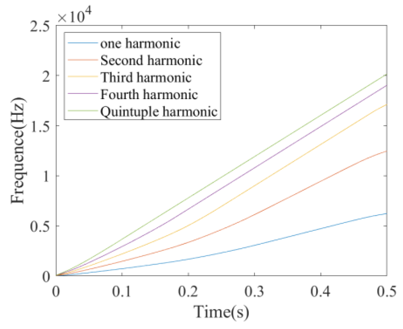
- Transient frequency phase conversion: The transient frequency represents the rotational speed of the complex plane vector argument, defined as the derivative of the phase. Hence, the estimate of the phase at each sample point becomes the integral of the transient frequency, that is, . As the D points are smooth, it is possible to use one of these points to represent the entire set of D points and achieve downsampling. After downsampling, the STFT is performed with a W point window, and the result is also smooth. Thus, within a certain window in the frequency domain, a single point can be used to represent the frequency of the whole window. Therefore, fr [m] = f [mDW], ϕr[m] is used as the sample point and the interpolation method is used to obtain the remaining phase values of ϕr[n] for the reconstruction of ϕr [n] = ϕ [nD]. As shown in Figure 2, the phases from the fundamental to the fifth harmonic are shown following the order from the bottom to the top.
2.2. Data Augmentation Scheme
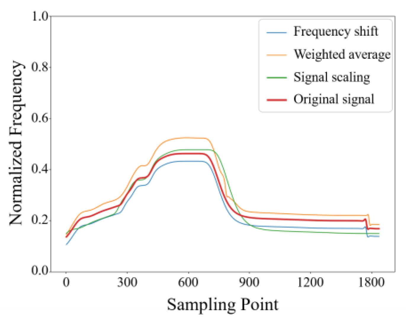
- Frequency shift: Since more attention is hereby paid to the waveform of the signal in signal generation, the frequency of the original signal is shifted up and down as a whole to expand the data of the signal. This method can improve the robustness of subsequent tasks to frequency changes in different signals, and can be expressed as follows:In Formula (5), fa′(t) represents the new signal, fa(t) denotes the original signal, and m is the base of the offset.
- Signal scaling: In the case of the inclusion of dolphin calls, there may be a Doppler shift, so signal spreading can be used for the simulation of this situation. In addition, this method can improve the feature extraction capability of the subsequent tasks [23], and the signal stretching can be expressed as follows:In Formula (6), fa′(t) represents the new signal, βfa(t) refers to the original signal, and β is the scaling factor.In the specific implementation, after normalizing the above two signals to a fixed length, their waveforms are the same. Thus, a small part of the signal at the beginning and end of the signal is cut out, and the signal is then normalized to the same length.
- Weighted average: In a data-limited scenario, the data distribution may not be complete, and the data elements of the same type of data may be far apart, which will cause trouble for subsequent tasks. Therefore, the weighted average of the signals between the same type of signals can be achieved [24]. Obtaining a new signal biased towards one of the signals also results in an average signal of the two signals. The method of weighted average makes the distribution of similar signals more uniform, and this method can be expressed as follows:In Formula (7), f(t) represents the new signal, fa(t) fb(t) denotes the same category in the original signal, and μ refers to the weight.
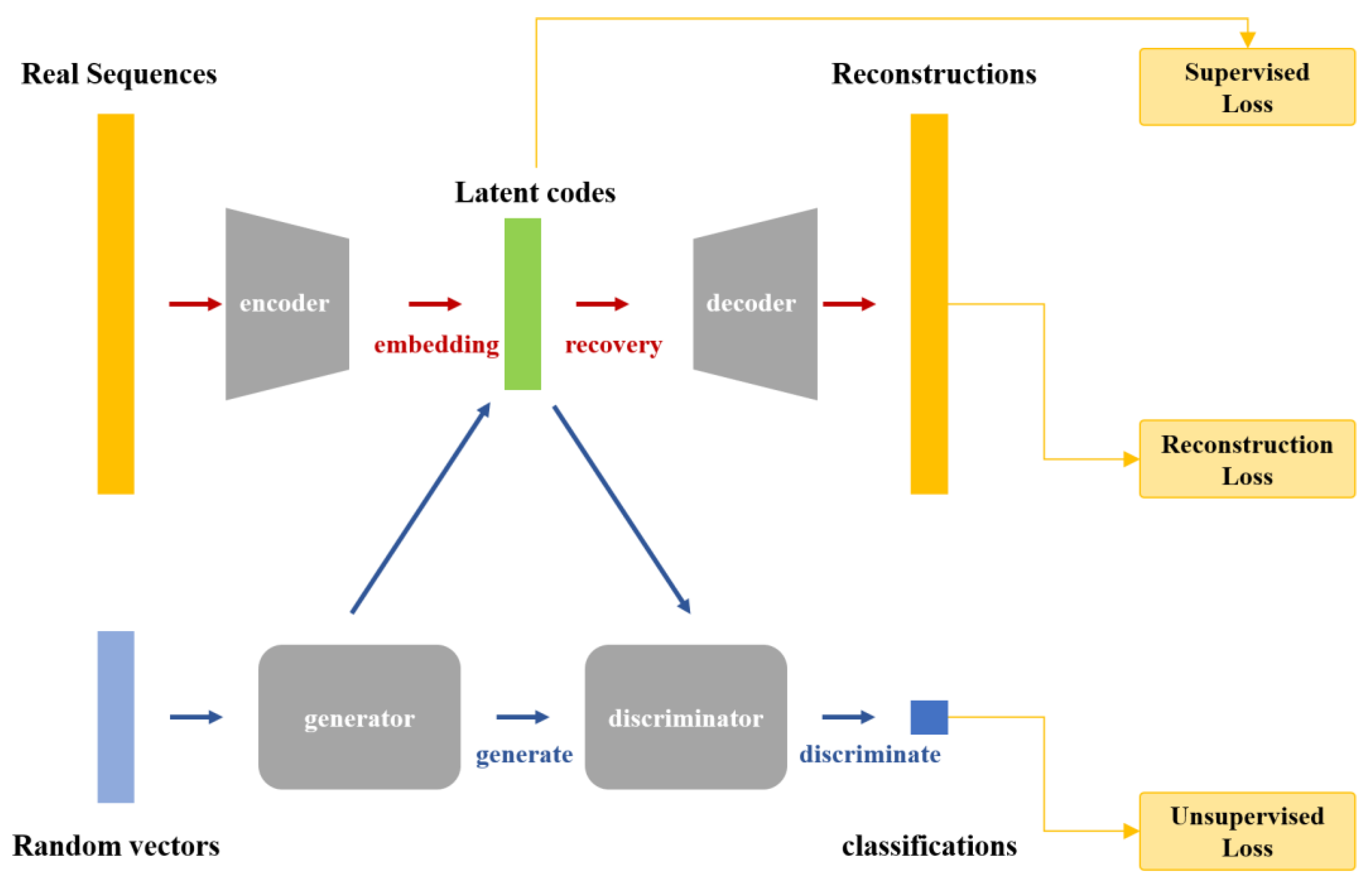
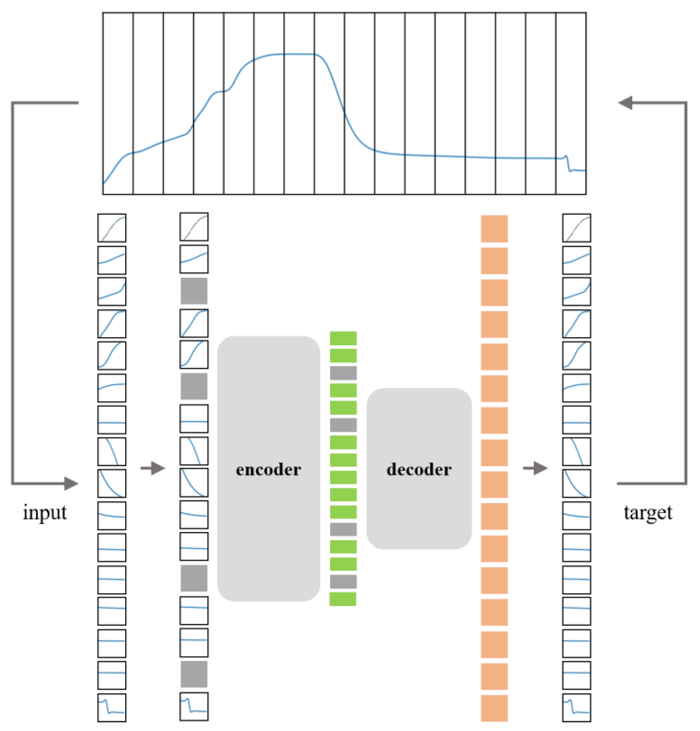
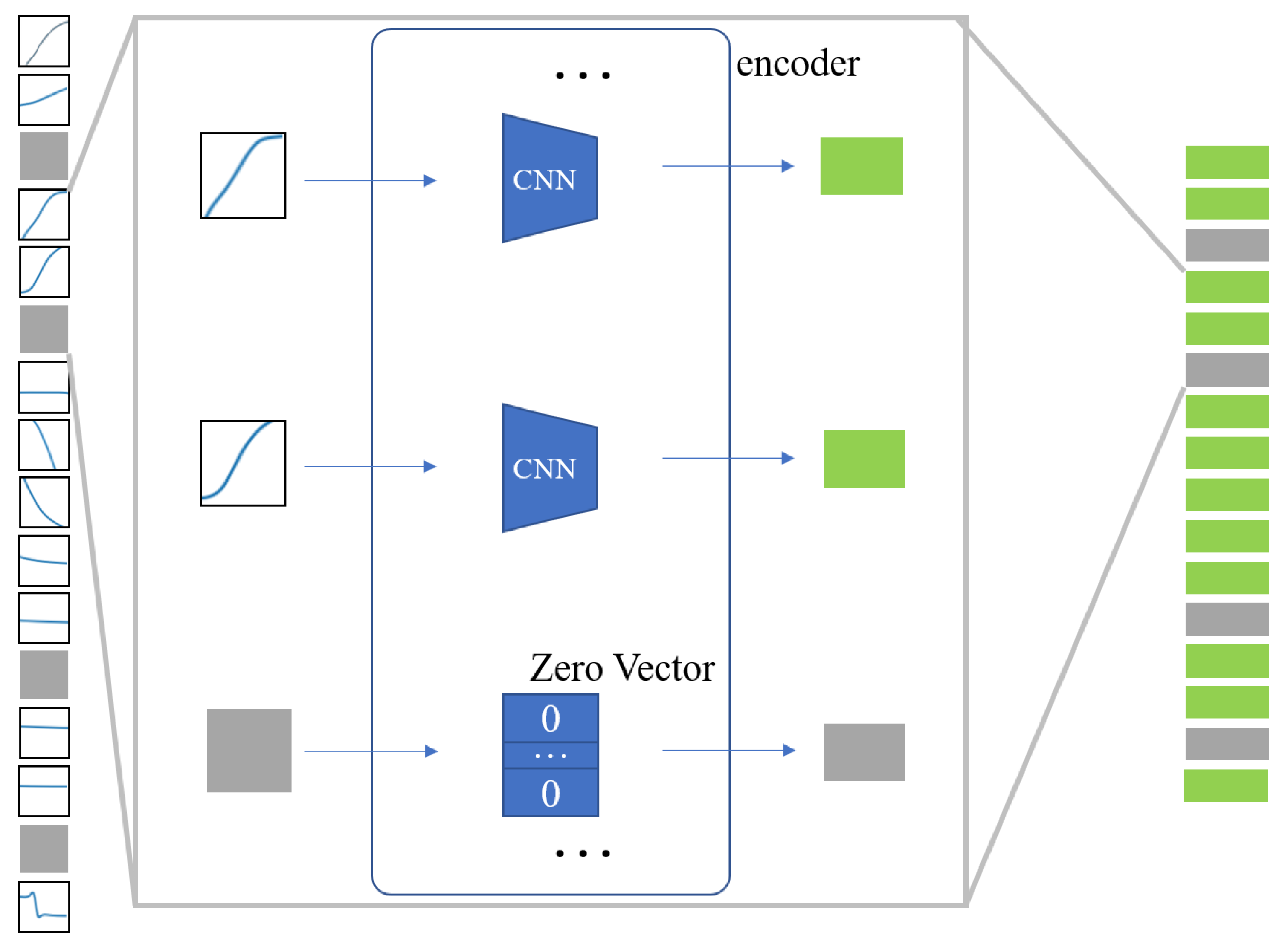
2.3. Proposed Method
3. Data and Implementation
3.1. Dataset
3.2. Implementation Detail
4. Experiments and Analysis
4.1. Evaluation Metrics
4.2. Evaluation Results
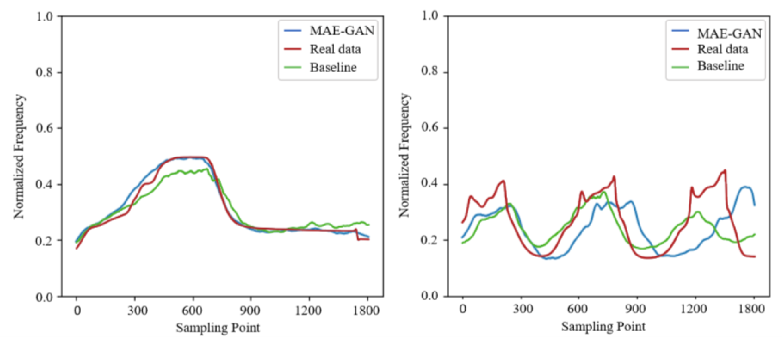
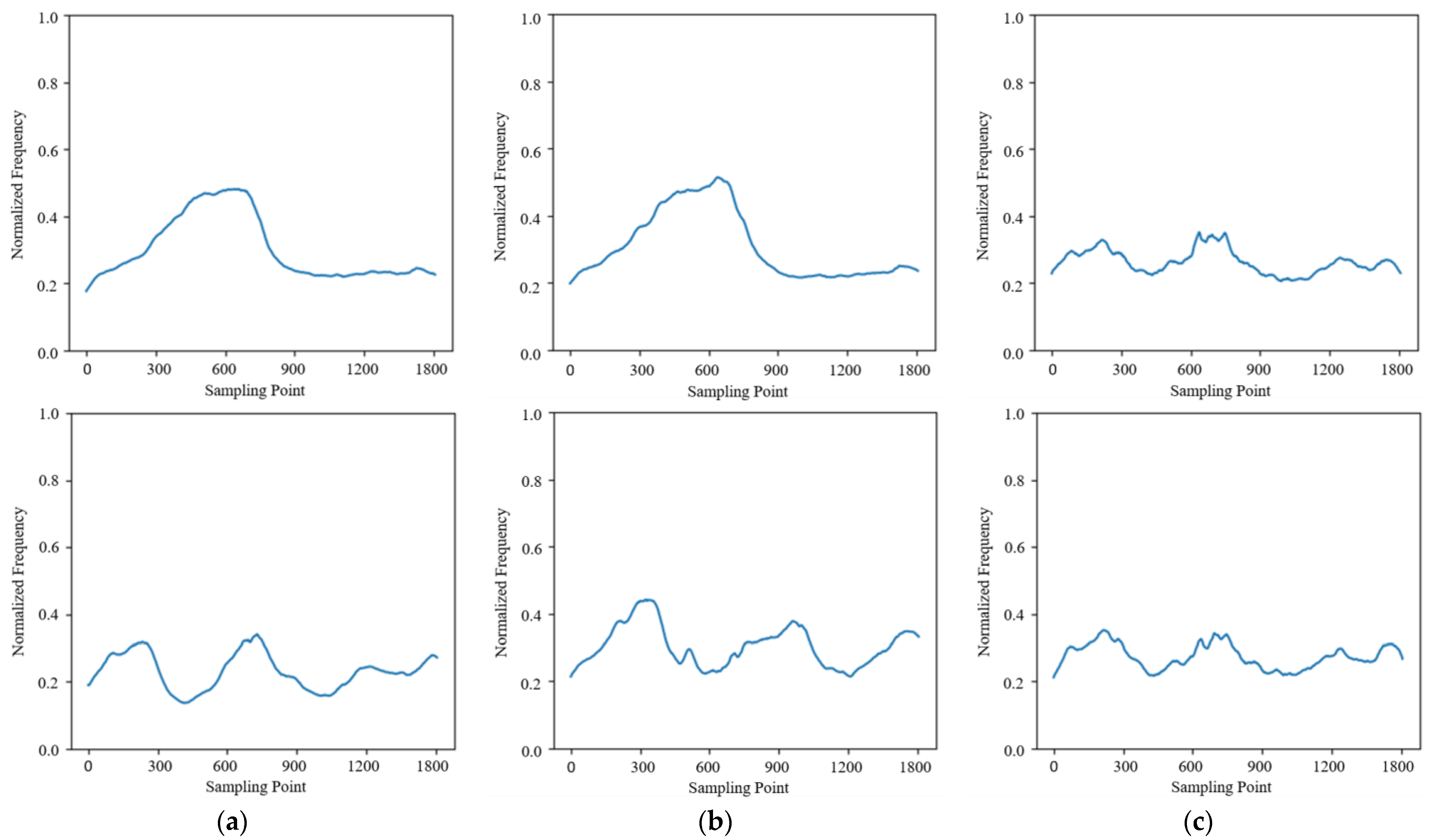
4.2.1. Raw Data
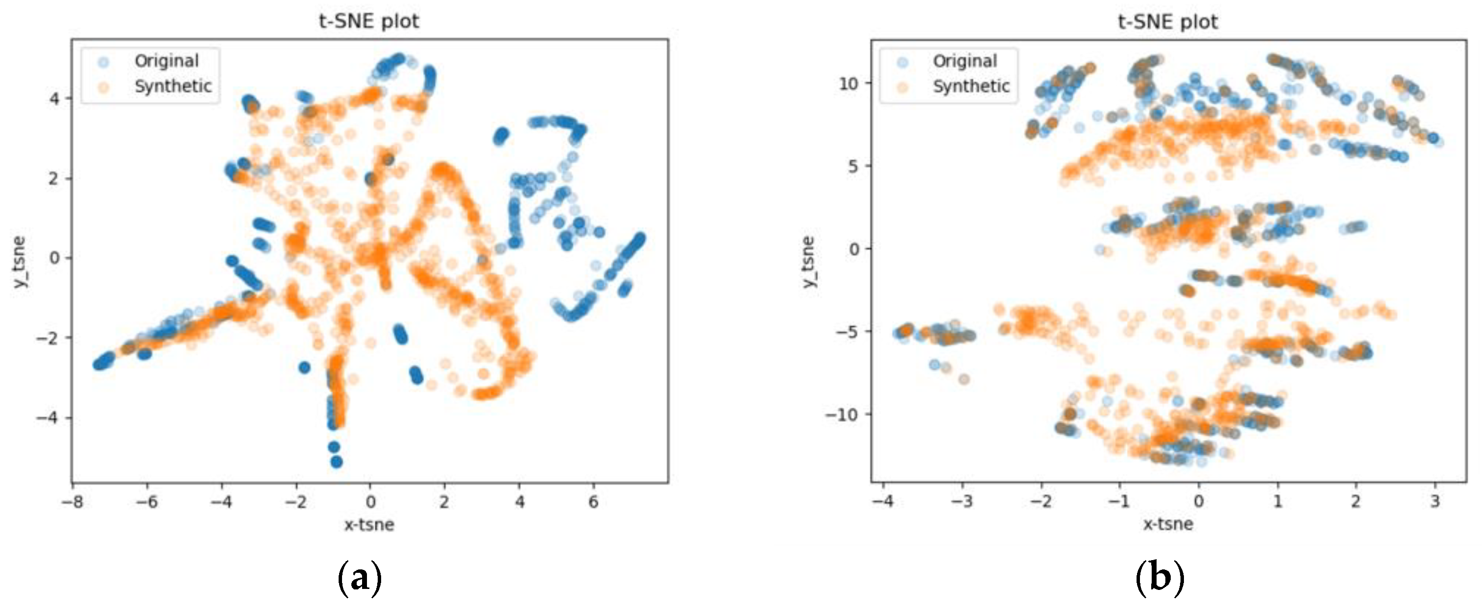
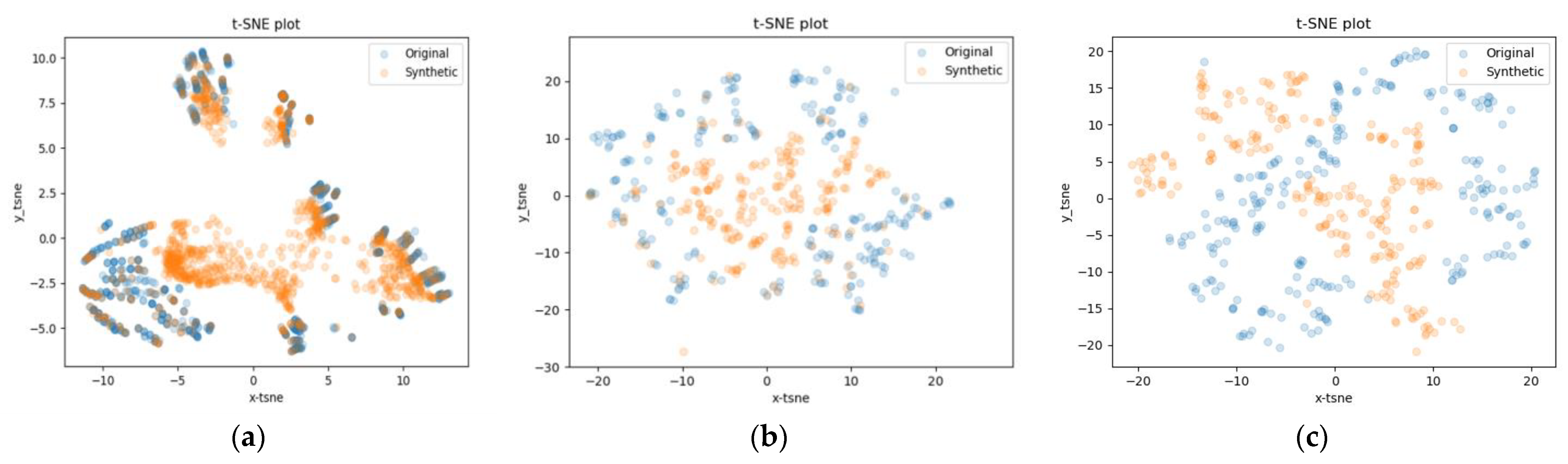
4.2.2. t-SNE
4.2.3. Discriminative Score
4.2.4. Space and Time Complexity
4.3. Ablation Experiment
5. Conclusions
Author Contributions
Funding
Institutional Review Board Statement
Informed Consent Statement
Data Availability Statement
Conflicts of Interest
References
- Li, C.; Jiang, J.; Wang, X.; Sun, Z.; Li, Z.; Fu, X.; Duan, F. Bionic Covert Underwater Communication Focusing on the Overlapping of Whistles and Clicks Generated by Different Cetacean Individuals. Appl. Acoust. 2021, 183, 108279. [Google Scholar] [CrossRef]
- Jiang, J.; Sun, Z.; Duan, F.; Fu, X.; Wang, X.; Li, C.; Liu, W.; Gan, L. Synthesis and Modification of Cetacean Tonal Sounds for Underwater Bionic Covert Detection and Communication. IEEE Access 2020, 8, 119980–119994. [Google Scholar] [CrossRef]
- Gregorietti, M.; Papale, E.; Ceraulo, M.; de Vita, C.; Pace, D.S.; Tranchida, G.; Mazzola, S.; Buscaino, G. Acoustic Presence of Dolphins through Whistles Detection in Mediterranean Shallow Waters. J. Mar. Sci. Eng. 2021, 9, 78. [Google Scholar] [CrossRef]
- Kipnis, D.; Diamant, R. Graph-Based Clustering of Dolphin Whistles. IEEE/ACM Trans. Audio Speech Lang. Process. 2021, 29, 2216–2227. [Google Scholar] [CrossRef]
- Li, P.; Liu, X.; Palmer, K.J.; Fleishman, E.; Gillespie, D.; Nosal, E.-M.; Shiu, Y.; Klinck, H.; Cholewiak, D.; Helble, T.; et al. Learning Deep Models from Synthetic Data for Extracting Dolphin Whistle Contours. In Proceedings of the 2020 International Joint Conference on Neural Networks (IJCNN), Glasgow, UK, 19–24 July 2020; pp. 1–10. [Google Scholar]
- Lin, C.-F.; Chung, Y.-C.; Zhu, J.-D.; Chang, S.-H.; Wen, C.-C.; Parinov, I.A.; Shevtsov, S.N. The Energy Based Characteristics of Sperm Whale Clicks Using the Hilbert Huang Transform Analysis Method. J. Acoust. Soc. Am. 2017, 142, 504. [Google Scholar] [CrossRef]
- Yan, S.; Zhou, X.; Hu, J.; Hanly, S.V. Low Probability of Detection Communication: Opportunities and Challenges. IEEE Wirel. Commun. 2019, 26, 19–25. [Google Scholar] [CrossRef]
- van der Merwe, J.R.; du Plessis, W.P.; Maasdorp, F.D.V.; Cilliers, J.E. Introduction of Low Probability of Recognition to Radar System Classification. In Proceedings of the 2016 IEEE Radar Conference (RadarConf), Philadelphia, PA, USA, 2–6 May 2016; pp. 1–5. [Google Scholar]
- Stove, A.G.; Hume, A.L.; Baker, C.J. Low Probability of Intercept Radar Strategies. IEE Proc. Radar Sonar Navig. 2004, 151, 249–260. [Google Scholar] [CrossRef]
- Cubuk, E.D.; Zoph, B.; Mane, D.; Vasudevan, V.; Le, Q.V. AutoAugment: Learning Augmentation Policies from Data. arXiv 2019, arXiv:1805.09501. [Google Scholar]
- Cubuk, E.D.; Zoph, B.; Shlens, J.; Le, Q.V. Randaugment: Practical Automated Data Augmentation with a Reduced Search Space. In Proceedings of the IEEE/CVF Conference on Computer Vision and Pattern Recognition (CVPR) Workshops, Seattle, WA, USA, 14–19 June 2020; pp. 702–703. [Google Scholar]
- Srivastava, N.; Hinton, G.; Krizhevsky, A.; Sutskever, I.; Salakhutdinov, R. Dropout: A Simple Way to Prevent Neural Networks from Overfitting. J. Mach. Learn. Res. 2014, 15, 1929–1958. [Google Scholar]
- Zhang, H.; Cisse, M.; Dauphin, Y.N.; Lopez-Paz, D. Mixup: Beyond Empirical Risk Minimization. arXiv 2018, arXiv:1710.09412. [Google Scholar]
- Yun, S.; Han, D.; Oh, S.J.; Chun, S.; Choe, J.; Yoo, Y. CutMix: Regularization Strategy to Train Strong Classifiers with Localizable Features. In Proceedings of the IEEE/CVF International Conference on Computer Vision (ICCV), Seoul, Republic of Korea, 27 October–2 November 2019. [Google Scholar]
- Goodfellow, I.; Pouget-Abadie, J.; Mirza, M.; Xu, B.; Warde-Farley, D.; Ozair, S.; Courville, A.; Bengio, Y. Generative Adversarial Networks. Commun. ACM 2020, 63, 139–144. [Google Scholar] [CrossRef]
- Li, Y.; Zhang, R.; Lu, J.; Shechtman, E. Few-Shot Image Generation with Elastic Weight Consolidation. arXiv 2020, arXiv:2012.02780. [Google Scholar]
- Li, K.; Zhang, Y.; Li, K.; Fu, Y. Adversarial Feature Hallucination Networks for Few-Shot Learning. In Proceedings of the IEEE/CVF Conference on Computer Vision and Pattern Recognition, Seattle, WA, USA, 13–19 June 2020; pp. 13470–13479. [Google Scholar]
- Subedi, B.; Sathishkumar, V.E.; Maheshwari, V.; Kumar, M.S.; Jayagopal, P.; Allayear, S.M. Feature Learning-Based Generative Adversarial Network Data Augmentation for Class-Based Few-Shot Learning. Math. Probl. Eng. 2022, 2022, e9710667. [Google Scholar] [CrossRef]
- Xiao, J.; Li, L.; Wang, C.; Zha, Z.-J.; Huang, Q. Few Shot Generative Model Adaption via Relaxed Spatial Structural Alignment. In Proceedings of the IEEE/CVF Conference on Computer Vision and Pattern Recognition, Nashville, TN, USA, 20–25 June 2022; pp. 11204–11213. [Google Scholar]
- Sinha, A.; Song, J.; Meng, C.; Ermon, S. D2C: Diffusion-Decoding Models for Few-Shot Conditional Generation. In Proceedings of the Advances in Neural Information Processing Systems, Virtual, 6–14 December 2021; Curran Associates, Inc.: Cambridge, MA, USA, 2021; Volume 34, pp. 12533–12548. [Google Scholar]
- Hazra, D.; Byun, Y.-C. SynSigGAN: Generative Adversarial Networks for Synthetic Biomedical Signal Generation. Biology 2020, 9, 441. [Google Scholar] [CrossRef]
- Zhang, L.; Huang, H.-N.; Yin, L.; Li, B.-Q.; Wu, D.; Liu, H.-R.; Li, X.-F.; Xie, Y.-L. Dolphin Vocal Sound Generation via Deep WaveGAN. J. Electron. Sci. Technol. 2022, 20, 100171. [Google Scholar] [CrossRef]
- Varghese, T.; Ophir, J. Enhancement of Echo-Signal Correlation in Elastography Using Temporal Stretching. IEEE Trans. Ultrason. Ferroelectr. Freq. Control 1997, 44, 173–180. [Google Scholar] [CrossRef]
- Forestier, G.; Petitjean, F.; Dau, H.A.; Webb, G.I.; Keogh, E. Generating Synthetic Time Series to Augment Sparse Datasets. In Proceedings of the 2017 IEEE International Conference on Data Mining (ICDM), New Orleans, LA, USA, 18–21 November 2017; pp. 865–870. [Google Scholar]
- Lu, J.; Yi, S. Autoencoding Conditional GAN for Portfolio Allocation Diversification. AEF 2022, 9, 55. [Google Scholar] [CrossRef]
- Zhang, Q.; Lin, J.; Song, H.; Sheng, G. Fault Identification Based on PD Ultrasonic Signal Using RNN, DNN and CNN. In Proceedings of the 2018 Condition Monitoring and Diagnosis (CMD), Perth, WA, Australia, 23–26 September 2018; pp. 1–6. [Google Scholar]
- He, K.; Chen, X.; Xie, S.; Li, Y.; Dollár, P.; Girshick, R. Masked Autoencoders Are Scalable Vision Learners. In Proceedings of the IEEE/CVF Conference on Computer Vision and Pattern Recognition (CVPR), New Orleans, LA, USA, 18–24 June 2022; pp. 16000–16009. [Google Scholar]
- Vaswani, A.; Shazeer, N.; Parmar, N.; Uszkoreit, J.; Jones, L.; Gomez, A.N.; Kaiser, Ł.; Polosukhin, I. Attention Is All You Need. In Proceedings of the Advances in Neural Information Processing Systems, Long Beach, CA, USA, 4–9 December 2017; Curran Associates, Inc.: Cambridge, MA, USA, 2017; Volume 30. [Google Scholar]
- Dosovitskiy, A.; Beyer, L.; Kolesnikov, A.; Weissenborn, D.; Zhai, X.; Unterthiner, T.; Dehghani, M.; Minderer, M.; Heigold, G.; Gelly, S.; et al. An Image Is Worth 16x16 Words: Transformers for Image Recognition at Scale. arXiv 2021, arXiv:2010.11929. [Google Scholar]
- Mao, J.; Zhou, H.; Yin, X.; Xu, Y.C.B.N.R. Masked Autoencoders Are Effective Solution to Transformer Data-Hungry. arXiv 2023, arXiv:2212.05677. [Google Scholar]
- Zhong, Z.; Zheng, L.; Kang, G.; Li, S.; Yang, Y. Random Erasing Data Augmentation. Proc. AAAI Conf. Artif. Intell. 2020, 34, 13001–13008. [Google Scholar] [CrossRef]
- Sayigh, L.; Daher, M.A.; Allen, J.; Gordon, H.; Joyce, K.; Stuhlmann, C.; Tyack, P. The Watkins Marine Mammal Sound Database: An Online, Freely Accessible Resource. Proc. Mtgs. Acoust. 2016, 27, 040013. [Google Scholar] [CrossRef]
- Arora, S.; Hu, W.; Kothari, P.K. An Analysis of the T-SNE Algorithm for Data Visualization. In Proceedings of the Conference On Learning Theory, PMLR, Stockholm, Sweden, 6–9 July 2018; pp. 1455–1462. [Google Scholar]
- Pei, H.; Ren, K.; Yang, Y.; Liu, C.; Qin, T.; Li, D. Towards Generating Real-World Time Series Data. In Proceedings of the 2021 IEEE International Conference on Data Mining (ICDM), Auckland, New Zealand, 7–10 December 2021. [Google Scholar]
- Yoon, J.; Jarrett, D.; van der Schaar, M. Time-Series Generative Adversarial Networks. In Proceedings of the Advances in Neural Information Processing Systems, Vancouver, BC, Canada, 8–14 December 2019; Curran Associates, Inc.: Cambridge, MA, USA, 2019; Volume 32. [Google Scholar]


| Model | 1D CNN Layer § | Normalization | Activation | ||||||
|---|---|---|---|---|---|---|---|---|---|
| Layer | Convolution Method | Input Channels | Output Channels | Kernel Size | Stride | Padding | |||
| Encoder Block * | 1 | Conv1d | 6 | 32 | 8 | 1 | 0 | LayerNorm | LeakyReLu † |
| 2 | Conv1d | 32 | 64 | 8 | 1 | 0 | LayerNorm | ||
| 3 | Conv1d | 64 | 128 | 8 | 2 | 0 | LayerNorm | ||
| 4 | Conv1d | 128 | 64 | 5 | 1 | 0 | LayerNorm | ||
| Decoder | 1 | ConvTranspose1d | 64 | 512 | 8 | 2 | 0 | LayerNorm | LeakyReLu |
| 2 | ConvTranspose1d | 512 | 1024 | 8 | 2 | 0 | LayerNorm | LeakyReLu | |
| 3 | ConvTranspose1d | 1024 | 512 | 8 | 2 | 0 | LayerNorm | LeakyReLu | |
| 4 | ConvTranspose1d | 512 | 6 | 8 | 2 | 0 | LayerNorm | LeakyReLu | |
| 5 | Linear | 602 | 512 | - | - | - | - | LeakyReLu | |
| 6 | Linear | 512 | 256 | - | - | - | - | LeakyReLu | |
| 7 | Linear | 256 | 512 | - | - | - | - | Sigmoid | |
| CWGAN-GP- generator | 1 | ConvTranspose1d | 100 | 512 | 4 | 1 | 0 | LayerNorm | ReLu |
| 2 | ConvTranspose1d | 512 | 256 | 4 | 2 | 1 | LayerNorm | ReLu | |
| 3 | ConvTranspose1d | 256 | 128 | 4 | 2 | 1 | LayerNorm | ReLu | |
| 4 | ConvTranspose1d | 128 | 64 | 4 | 2 | 1 | LayerNorm | ReLu | |
| 5 | Conv1d | 64 | 64 | 4 | 2 | 1 | LayerNorm | Tanh | |
| CWGAN-GP- Discriminator | 1 | Conv1d | 64 | 64 | 4 | 1 | 1 | LayerNorm | LeakyReLu |
| 2 | Conv1d | 64 | 128 | 4 | 2 | 1 | LayerNorm | LeakyReLu | |
| 3 | Conv1d | 128 | 256 | 4 | 2 | 1 | LayerNorm | LeakyReLu | |
| 4 | Conv1d | 256 | 512 | 4 | 2 | 1 | LayerNorm | LeakyReLu | |
| 5 | Conv1d | 512 | 1 | 3 | 1 | 0 | - | - | |
| Method | Discriminative Score |
|---|---|
| Baseline model | 0.362 |
| MAE-GAN | 0.074 |
| Method | Param (M) | MFLOPs |
|---|---|---|
| MAE-GAN | 1.65 | 68.5 |
| Baseline model | 1.24 | 226.7 |
| Deep WAVEGAN | 3.73 | 86,951.3 |
| Method | Discriminative Score |
|---|---|
| Data augmentation without MAE | 0.21 |
| MAE without data augmentation | 0.84 |
| Without data augmentation and MAE | 0.92 |
Disclaimer/Publisher’s Note: The statements, opinions and data contained in all publications are solely those of the individual author(s) and contributor(s) and not of MDPI and/or the editor(s). MDPI and/or the editor(s) disclaim responsibility for any injury to people or property resulting from any ideas, methods, instructions or products referred to in the content. |
© 2023 by the authors. Licensee MDPI, Basel, Switzerland. This article is an open access article distributed under the terms and conditions of the Creative Commons Attribution (CC BY) license (https://creativecommons.org/licenses/by/4.0/).
Share and Cite
Wang, H.; Wu, X.; Wang, Z.; Hao, Y.; Hao, C.; He, X.; Hu, Q. Low-Resource Generation Method for Few-Shot Dolphin Whistle Signal Based on Generative Adversarial Network. J. Mar. Sci. Eng. 2023, 11, 1086. https://doi.org/10.3390/jmse11051086
Wang H, Wu X, Wang Z, Hao Y, Hao C, He X, Hu Q. Low-Resource Generation Method for Few-Shot Dolphin Whistle Signal Based on Generative Adversarial Network. Journal of Marine Science and Engineering. 2023; 11(5):1086. https://doi.org/10.3390/jmse11051086
Chicago/Turabian StyleWang, Huiyuan, Xiaojun Wu, Zirui Wang, Yukun Hao, Chengpeng Hao, Xinyi He, and Qiao Hu. 2023. "Low-Resource Generation Method for Few-Shot Dolphin Whistle Signal Based on Generative Adversarial Network" Journal of Marine Science and Engineering 11, no. 5: 1086. https://doi.org/10.3390/jmse11051086