Climatic Trend of Wind Energy Resource in the Antarctic

Abstract

Wind energy resource is an important support for the sustainable development of Antarctica. The evaluation of wind energy potential determines the feasibility and economy of wind power generation in Antarctica, among which mastering the variation rule of wind energy resource is the key to realizing the effective utilization of polar wind energy. Based on the 6-h ERA-5 reanalysis data of ECMWF from January 1981 to December 2020, this paper systematically analyzed the long-term variation trend of Antarctic wind energy resource by using the climate statistical analysis method and the least square fitting, with the comprehensive consideration of a series of key indicators such as Wind Power Density, Effective Wind Speed Occurrence, Energy Level Occurrence, and Stability. The results show that it indicates a positive trend for wind power density (0.5~2 W × m⁻² × a⁻¹), effective wind speed occurrence (2~3%/a), energy level occurrence (0.1~0.2%/a), and coefficient of variation (−0.005/a) in the South Pole—Kunlun station and the central region of Queen Maud land. The westerly belt exhibits a decreasing index (−0.5%/a) in terms of stability trend, indicating a positive potential. Kemp Land, the Ross Island—Balleny Islands waters show shortages in all indicators. The wind power density in the Antarctic region is stronger in spring and summer than in autumn and winter, with the weakest in autumn. Based on the above indicators, the variation trend in the East Antarctic coast, Wilhelm II Land—Wilkes Land, the South Pole—Kunlun station, and the westerlies is generally superior.

1. Introduction

With the advancement of globalization, the two poles have garnered increased attention from countries and regions alike. Antarctica is home to 80% of the world’s freshwater resources and boasts the largest reserves of oil and coal globally. As the planet’s “cold source”, Antarctica is one of the sensitive areas for climate change, and its shifts serve as a “magnifying glass” for global climate anomalies [1]. China’s 14th Five-Year Plan specifically proposes to fortify its participation in the protection and utilization of Antarctica. The United States proposes to “maintain an active and influential presence in the Antarctic region”, while Australia issues a 10-year Antarctic science strategic plan to emphasize the significance of Antarctica and Australia’s position in this area. The UK mainly deepens its understanding and participation in the governance of Antarctica from the strategic perspectives of scientific research, heritage preservation, and environmental conservation. Simmonds and Jacka used the 20-year sea ice data and the Southern Oscillation Index provided by NOAA and found a correlation between the sea ice in the Indian Ocean, Pacific Ocean, and Ross Sea and the Southern Oscillation [2]. Using ERA40 data to evaluate the IPCC AR4 model, Kolstad and Bracegirdle discovered that the transportation of cold air from polar regions will result in outbreaks of cold air at the middle and low latitudes, which affects climate change. The study highlights the importance of considering these mechanisms in climate models in order to accurately predict future climatic trends and variations [3]. Research has shown that changes in sea ice levels near Antarctica cause regional atmospheric circulation anomalies, which affect weather and climate at the middle and low latitudes [4,5]. With ERA-interim data, Yu and Zhong analyzed the correlation between strong wind events and climate patterns in Antarctica, indicating that the higher frequency of strong wind events in East Antarctica is associated with positive anomalies of surface temperature and negative anomalies of cyclones. Additionally, they noted that compared with ENSO, the interannual variation of strong wind events is associated with SAM [6]. Previous studies have shown that Antarctic sea ice changes affect precipitation in East Asia [7,8,9,10]. Therefore, exploration in Antarctica is essential. The wind near the surface of Antarctica is one of the strongest on the planet, known as the “wind pole”. Due to the difficulty of energy transportation in Antarctica, led by the strong winds, the need for energy for research stations and shipping lanes is a significant concern. To address this challenge, China began using an unmanned polar energy system at Taishan Station in 2019, which requires five tons of jet fuel annually to keep the station supplied with electricity. The use of fossil fuels in such a sensitive environment has raised concerns about gas emissions and environmental pollution, which poses new challenges to the Antarctic ecology. Located in the southernmost part, Antarctica has a simple ecological structure, which makes it particularly vulnerable to rising temperatures resulting from excessive greenhouse gas emissions. This warming leads to further emissions, causing a vicious cycle that threatens the delicate regional ecosystem [11]. However, the Belgian-funded Princess Elisabeth Station, constructed in 2009, is revered as the “greenest research station in Antarctica”. As the first-ever Antarctic research station to run solely on wind and solar power, it is also the first “zero-carbon” research station in the world. In response to the newly proposed “carbon peak” and “carbon neutral” objectives, the construction of a “zero carbon emission” research station in Antarctica showcases the importance of clean energy. China aims to support the development of offshore wind power facilities and promotes the implementation in deep water and distant shore areas. Leveraging both offshore and onshore wind power in Antarctica can provide a sustainable source of clean energy for research stations and shipping routes in the region, marking a significant step forward in the continent’s progress.

Resource Evaluation should be ahead of Resource Development. The long-term trend of energy also plays a key role in assessment and development and site construction in the region. Komal evaluated the wind energy of Pakistan by comparing the SODAR data with the measured data and found that it is economically feasible to use SODAR data to evaluate wind energy [12]. Saulat evaluated and predicted Pakistan’s wind energy resources based on the previous studies using site data and pointed out that Pakistan owns optimistic wind energy resources, but the development is slow, and put forward decision-making suggestions on the utilization of wind energy to develop resources [13]. Gao et al. analyzed the distribution characteristics and overall variation trend of the wind power density in China’s coastal and surrounding waters, pointing out that China’s coastal wind energy enrichment areas are in Taiwan—South China Sea, and most of the sea areas show an increasing trend year by year [14]. Onea et al. (2019) analyzed the wind energy distribution of Romania’s coastal areas with ERA-interim wind field data and pointed out that the best location for wind power projects is in the north of the Black Sea [15]. Rusu predicted the wind energy resources of the Black Sea coast in the next 30 years with the data provided by the climate wind model RCA4 [16]. Lima analyzed the influences of the western waters in South Africa on the current and future climate, predicted the variation trend of offshore wind power density in the 21st century, and pointed out that the wind power density in the west of South Africa is the highest and increases year by year [17]. Spezakis and Xydis studied the feasibility of transporting offshore wind power through pipelines for hydrogen transmission in the western Gulf of Mexico according to the wind power plan and research on the infrastructure reconstruction proposed by the United States [18]. Carreno et al. analyzed wind power density and capacity factors in the Iberian Peninsula with ERA-20 and ERA-5 wind field data and pointed out that wind power density and capacity factors and other indicators are the highest in the Atlantic region and the Gulf of Lyon, and the wind energy resources are abundant [19]. Wen et al. analyzed the spatial and temporal distribution of wind resources in the South China Sea and evaluated the potential of offshore wind energy with JRA-55 wind field data, and pointed out that the long-term trend of wind energy in the South China Sea has been basically flat in the past 50 years [20]. Predicting the offshore wind energy in China’s coastal areas with CORDEX wind speed, Costoya et al. analyzed the wind power density, stability, risk, economy, and other factors and concluded that the wind power density in China’s coastal areas shows a declining trend, and most areas are rich in wind energy resources [21]. Decastro et al. ever analyzed the differences in the development status of offshore wind energy in Europe, China, and the United States and pointed out that in offshore wind energy development, Europe is currently in the leading position, China is developing rapidly, and the development trend of the United States depends on its laws and regulations [22]. Carvalho made use of two future climate scenarios of CMIP6 to predict the variation of wind energy resources in Europe and pointed out that the resources in the scattered areas would increase in the future but would decline in most areas of Europe [23]. Xydis ever used the measured data to study the wind energy in the central mountainous region of Greece and concluded that the wind energy in the mountainous region is conducive to the planning and construction of wind farms [24]. Zheng et al. conducted a study using 40 years of ERA5 data to analyze the evolution of global wind speed and wave height. They concluded that there is a positive growth trend, with stronger growth in the southern hemisphere than in the northern hemisphere. Additionally, the dominant regions are in the southern Indian Ocean and the tropical Pacific Ocean, which can provide a reference for the long-term planning of global wind and wave energy development [25]. Yu and Zhong used ERA-interim data and Self-Organizing Map technology to analyze the changing trend of surface wind speed in Antarctica and the Southern Ocean and revealed the changes in wind energy in Antarctica. They pointed out that the surface wind is stronger in East Antarctica and near the Trans-Antarctic Mountains, which is stronger in winter than in summer. Most regions show a significant growth trend [26]. Pourrahmani [27] made use of wind profile data in the Cohen region of Iran and alkaline electrolyzers to store excess electricity generated by turbines and pointed out that alkaline electrolyzers and proton-exchange membrane fuel cells can well store and back up the excess. Zahedi et al. [28,29] reviewed previous wind energy studies and used GIS software to evaluate the regional wind energy potential with the Multi-Criteria Decision-Making method to determine the location of wind power plants by considering elements such as environment, economy, and geography. Zahedi et al. [30] studied the fuel-cell–wind-power hybrid wind turbine system and assessed its environmental impact, pointing out that the system can effectively reduce the production of carbon dioxide and reduce the cost of wind power generation.

Predecessors have made important contributions to the study of the characteristics of Antarctic surface winds, variation causes, and the effects on global climate. Based on the data from Antarctic weather stations and the analysis of temporal and spatial characteristics of reanalysis datasets, the characteristics of wind speed changes are used to evaluate the wind energy in Antarctica to reveal the characteristics of wind energy.

However, due to factors such as threshold and stability of effective wind speed, wind energy is not the same as wind speed variation characteristics, which cannot well represent the changes in Antarctic wind energy. The purpose and novelty of this study are to make a direct statistical analysis of a series of key indicators of wind energy and calculate the long-term evolution trend of the whole set of key indicators of wind energy with the least square and regression analysis system. It is conducive to the direct grasp of wind energy and provides a scientific basis for the long-term planning of Antarctic wind energy development. The long-term variation trend of resources is closely related to its long-term planning [31,32,33,34]. Thus, the ERA-5 reanalysis data from the European Centre for Medium-Range Weather Forecasts (ECMWF) is used to study the historical variation trend of a series of indicators of wind energy resources in the Antarctic region in the hope of providing a scientific basis for the long-term planning of wind energy development and the construction of strategic support points and providing auxiliary decision making for the development and construction of wind energy in the Antarctic region, so as to increase the utilization of clean energy to promote the sustainable development in the Antarctic region.

2. Methodology and Data

2.1. Data

ERA-5 reanalysis wind field data (including 10 m meridional and zonal wind at sea surface) are from ECMWF, the spatial range covers the whole world, and the spatial resolution is 0.25° × 0.25° at atmospheric level. The spatial range selected in this study is 60° S~90° S, 180° W~180° E, and the time series is from 00:00 1 January 1959 to the present and is constantly updated. The time range selected in this study is from 00:00 1 January 1981 to 18:00 31 December 2020, and the time resolution is 6 h.

ERA-5 reanalysis wind field data is the fifth generation of reanalysis dataset following ERA-40 data and ERA-interim data. Compared with previous generations, ERA-5 data is the latest benchmark for reanalysis data [35], with a higher spatial and temporal resolution, improved model parameters, and data assimilation methods. Studies show that the overall accuracy of the ERA-5 data improves, including rainfall and tropical convection data [36,37], surface temperature data [38], surface solar radiation data [39], and wind field data [35].

2.2. Methods

With ERA-5 reanalysis data from ECMWF, this study adopts the offshore wind energy resource evaluation system established by Zheng et al. [40,41] to analyze the long-term trend of a series of key indicators of wind energy resources in the Antarctic region westward, including wind power density (WPD), effective wind speed occurrence (EWSO), energy level occurrence, and wind power density stability (coefficient of variation, monthly variability index, seasonal variability index). The trend of wind power density can be calculated as follows:

$$W=\frac{1}{2}\rho V^3.$$

(1)

In Formula (1), $W$ is wind power density (W/m²); $V$ is wind speed (m/s); $\rho$ is sea surface air density (kg/m³). When the altitude is less than 500 m, $\rho$ is 1.225 kg/m³.

Averaging the 6-h wind power density from 00:00 1 March 1981 to 18:00 31 March 1981 can obtain the average wind power density in March 1981 at each grid point of 0.25° × 0.25° in the Antarctic region. The average wind power density in Antarctica in March, April, and May in the last 40 years is obtained by the same method. Averaging wind power density in Antarctica in March, April, and May of 1981 can be obtained in Antarctica in the autumn of 1981 and autumns of the last 40 years. The variation trend of the wind power density of spring, summer, autumn, and winter and of the annual average in the Antarctic region under the average state in the last 40 years can be obtained through the least square fitting and regression analysis for the above 40-year wind power data in autumn. The shaded points indicate that the trend passes the 95% significance test. Trends in other wind energy indicators are also calculated in this way.

3. The Long-Term Trend

3.1. Wind Power Density

The annual variation trend of WPD (as shown in Figure 1e) is as follows: as a whole, there is no significant wind power density variation trend in the Southern Ocean and the West Antarctic. The areas with a significant increase trend are mainly distributed in the coastal areas of Queen Maud Land and Enderby Land in the East Antarctic and the areas near the Davis Station, and the increasing trend is relatively strong, which is up to 2 W × m⁻² × a⁻¹. The areas with a significant declining trend are mainly distributed near the Cape Adare, the Wilkes Land coast, Mac.Robertson Land, the Weddell Sea, and the Ross Sea, which is −0.5~−1 W × m⁻² × a⁻¹. It is worth noting that the declining trend near the Cape Adare and Mac.Robertson Land is relatively strong, which is up to −3 W × m⁻² × a⁻¹, and there is a generally static trend in the interior of the Antarctic continent. The positive wind-energy-change trend indicates the strengthening of resources. The negative change trend indicates the weakening of resources. Moreover, no significant change trend indicates stable resources. Increasing and steady wind power is beneficial to resource development.

The seasonal variation trend of WPD is as follows: in spring (Figure 1a), the areas with a significant increase are distributed in the southwest of the Showa Station, Enderby Land, Princess Elizabeth—Wilhelm II Land and Queen Mary Land (3~5 W × m⁻² × a⁻¹), while the areas with a significant decrease are mainly distributed in the vicinity of the Weddell Sea (−2 W × m⁻² × a⁻¹), northern Cape Adare and Southern Ocean-Pacific area (−4~−6 W × m⁻² × a⁻¹) and Kemp Land—Mac.Robertson Land (−5~−10 W × m⁻² × a⁻¹). There is a significantly stable trend in the central part of the Antarctic continent.

In summer (Figure 1b), the areas with a significant decrease are mainly distributed in the Amundsen Sea and its coastal areas (−2 W × m⁻² × a⁻¹) and near the Cape Adare (−6 W × m⁻² × a⁻¹). The areas with a significant increase are distributed in the Norwegian Cape (4~6 W × m⁻² × a⁻¹), near the Showa Station and the Lazarev Sea (2 W × m⁻² × a⁻¹). There is a significant stable trend near the South Pole and in the south of Princess Elisabeth—Wilhelm II Land and north of the Weddell Sea.

In autumn (Figure 1c), the areas with a significant increase are located near the Norwegian Cape (5–10 W × m⁻² × a⁻¹). The areas with a significant decline are near the coast of Marie Byrd Land (−15~−10 W × m⁻² × a⁻¹), near the Roosevelt Peninsula (−5 W × m⁻² × a⁻¹), from the Ross Island to the Balerny Islands (−10~−25 W × m⁻² × a⁻¹), and near the Dumont d’Urville Station (−10~−20 W × m⁻² × a⁻¹). The maximum decrease trend of Cape Adare is −25 W × m⁻² × a⁻¹. There is a stable trend near the Queen Maud Land—Kemp land and the Wilhelm II land.

In winter (Figure 1d), it is dominated by the significantly declining areas, which are mainly distributed in the vicinity of the Weddell Sea and the Ross Sea (−5 W × m⁻² × a⁻¹). The extreme value center of −10 W × m⁻² × a⁻¹ appears across the Transantarctic Mountains, and the significantly declining areas of −5~−10 W × m⁻² × a⁻¹ also appear near the Kempe Land and the Dumont d’Urville Station. The areas with a significant increase are located near the Enderby Land and the Prydz Bay (6~8 W × m⁻² × a⁻¹).

By comparing the variation trends of WPD in different seasons and years, it can be found that the variation trends of WPD in different regions are dominated by different seasons: the stable trend near the South Pole is dominated by spring and summer, and in Elizabeth Land it is dominated by summer, and the significantly increasing trend in Queen Maud Land and Enderby Land and near the Davis Station is dominated by spring. The significantly decreasing areas of 110° E~180° are manifested in four seasons, and the decreasing trend in the Ross Sea is dominated by winter, and in the Weddell Sea it is dominated by winter and spring. The largest increase in surface temperature is observed in East Antarctica, primarily due to the annual cycle of surface temperature and its associated inversion in this area [42]. The changing trend is also influenced by topography, showing a positive trend in the coastal areas of the Southeast Pole but a weak or negative trend in the plain areas of East Antarctica, which is caused by the evolution trend of wind energy and the blocking of topography.

3.2. Effective Wind Speed Occurrence

With the definition of effective wind speed occurrence proposed by Zheng et al. [40,41], it is believed that the wind speed, which is 5~25 m/s is conducive to the collection and conversion of wind energy resources.

The annual variation trend of EWSO (Figure 2e) is as follows: the Southern Ocean as a whole shows a decreasing trend year by year. The areas which pass the significance tests are in the vicinity of the Bellingshausen Sea (−0.1%/a), the Ross Sea, and the Cape Adare (−0.2~−0.3%/a), and in northern Cape Adare and northern Wilkes Land (−1.5~−2.5%/a). The areas with a significant increase are around the South Pole Kunlun Station (2~2.5%/a), in the middle of Queen Maud Land and in Wilhelm II Land (0.2~0.3%/a). The mainland of the East Antarctic (0.1%/a) showed a positive trend, indicating a positive increase in the EWSO of this area in the past 40 years, and this area has great potential for wind energy resources and certain development values. Otherwise, it means that the availability of this area is small. When developing wind energy in this area, comprehensive consideration should be given to the temporal and spatial characteristics for selection.

The seasonal variation trend of EWSO is as follows: in spring (Figure 2a), the areas with a significantly increasing trend are distributed in the East Antarctic (0.3~0.5%/a), south Wilhelm II—Queen Mary Land and south Wilkes Land (0.1~0.5%/a) and around Enderby—Queen Maud Land (0.1~0.5%/a). The areas with a significantly decreasing trend are distributed in the Southern Ocean, including the Weddell Sea and the Bellingshausen Sea (−0.3~−0.5%/a), the Southern Ocean-Pacific area (−0.3%/a), the northern area of the Cape Adare Casey Station (−0.3~−0.5%/a), and the northern area of the Roosevelt Island (−0.3~−0.6%/a). In summer (Figure 2b), the distribution of significantly increasing areas is basically unchanged. The areas with a significant decrease are located in Ellsworth Land (−0.2~−0.4 %/a) and the Voyeykov Ice Shelf—Shackleton Ice Shelf coastal area (−0.3%/a). In autumn (Figure 2c), the areas with a positive trend are distributed in the South Pole and Antarctica peninsula. The effective wind speed occurrence in Antarctica shows a decreasing trend. The areas with a significant decrease are mainly distributed in Marie Byrd Land (−0.4%/a), including Roosevelt Island and Dart Island, and in the waters around the Ross Island-Balerny Islands (−0.4~−0.6%/a), the East Pole coast (−0.2%/a), and the Lazarev Sea (−0.4%/a). The effective wind speed occurrence in the Princess Elizabeth and Queen Mary land, which increases significantly in other seasons, tends to be static in autumn. In winter (Figure 2d), it continues to show a decreasing trend, with decreasing areas of −0.1~−0.2%/a in the Southern Ocean, −0.4%/a near the Balerny Islands, and −0.4~−0.6%/a in the Bellingshausen Sea, the Weddell Sea, the Ross Sea, and the Lazarev Sea—Haakon VII Sea. There is a significantly increasing area of 0.2%/a along Mac.Robertson Land and the Davis Station.

By comparing EWSO variation trends in different seasons and years, it can be found that EWSO variation trends in different regions are dominated by different seasons. The increasing trend near the South Pole Kunlun Station and Wilhelm II Land is dominated by spring and summer, and near Queen Maud Land it is dominated by spring. The significantly decreasing areas of the Southern Ocean are shown in spring and winter, and the decreasing trend near the Casey Station is shown in four seasons. The evolution trend of EWSO in the Antarctic is mainly related to the topography. Due to the radiative cooling of the air near the slope, the air sinks and forms a strong descending wind [43,44]. In autumn and winter, the changing trend is not obvious due to the relatively stable temperature.

3.3. Energy Level Occurrence

The occurrence of different energy levels is an important index to measure the abundance of wind energy resources. The key index of wind energy level occurrence proposed by Zheng et al. [40,41] is used to describe the abundance of wind energy. In this study, ALO, RLO, and SLO are selected to describe the availability of wind power density in the Antarctic region. ALO (Available Level Occurrence) is defined as an energy level occurrence above 100 W/m², RLO (Rich Level Occurrence) is defined as an energy level occurrence above 200 W/m², and SLO (Superb Level Occurrence) is defined as an energy level occurrence above 400 W/m².

3.3.1. Available Level Occurrence

The annual variation trend of ALO (Figure 3e) is as follows: ALO is one of the indicators to determine whether wind energy is available, and the positive trend is distributed in the East Antarctic (0.2%/a), and there is a significantly decreasing center (−0.15%/a) only near the waters of the Cape Adare and Balerny Islands. Other regions fail to pass the significance test of 0.05, with no significant variation trend. It is speculated that the reason may be that the Antarctic region is rich in wind energy resources, and the wind speed is stable. The wind power density in all regions is basically higher than 100 W/m² throughout the year, so the long-term variation trend is not significant. The evolution trend of ALO is similar to that of EWSO. In essence, both of them count the limited conditions, while availability counts the wind speed, and ALO counts the wind power density. The reason for the similarity may be that wind speed at sea is relatively high, and the corresponding area in EWSO exactly meets the conditions of ALO.

The seasonal variation trend of ALO is as follows: in spring (Figure 3a), the significantly increasing areas are mainly distributed in the East Antarctic (0.2~0.4%/a), Wilhelm II Land—Wilkes Land (0.1~0.4%/a), and Enderby Land—Queen Maud Land (0.1~0.4%/a). Meanwhile, the significantly decreasing areas are found in the northern Roosevelt Island (−0.3~−0.5%/a), most areas of the northern Ross Sea—Voyeykov Ice Shelf (−0.2~−0.4%/a). In summer (Figure 3b), the significantly increasing areas are located near the South Pole (0.2–0.3%/a), south Kunlun Station—Wilhelm II Land—Wilkes Land (0.1–0.2%/a), and the Lazarev Sea (0.2%/a). In contrast, the significantly decreasing areas are located near the Voyeykov Ice Shelf and the Shackleton Ice Shelf (−0.2~−0.3%/a) and south of the Abbot Ice Shelf (−0.2~−0.3%/a). In autumn (Figure 3c), the significantly increasing areas are found near the South Pole (0.2%/a), the Princess Elizabeth Land (0~0.2%/a), and Enderby Land (0.1%/a). Meanwhile, the significantly decreasing areas are mainly distributed in the Southern Ocean (−0.1~−0.2%/a), the waters between the Ross Island and the Balerny Islands (−0.3~−0.6%/a), Marie Byrd Land and Roosevelt Island (−0.3~−0.4%/a), and the Kunlun Station (−0.3%/a). In winter (Figure 3d), there is a decreasing trend in the Antarctic as a whole, and the ALO is −0.2%/a in most areas of the Southern Ocean. There is a declining, large-value area of −0.3~0.4%/a in the Bellingshausen Sea, the Weddell Sea, the Haakon VII Sea, and north of the Balerny Islands, and a declining area of −0.3~−0.5%/a in the Ross Sea. Furthermore, there is an increasing area of 0.1%/a in the central region of the Queen Maud Land and the sea area in the north of Mawson Station—Davis Station. By comparing the variation trends of EWSO in different seasons and years, it can be found that the declining areas in the north of Cape Adare are reflected in spring and winter.

In contrast to seasonal variation trends, the evolution trend of ALO in the East Antarctic continent is significantly affected by topography, while the ALO in East Antarctica presents a barrier along the outer mountains of the continent, with a positive trend within the barrier and few changes outside. This may be due to the greater wind energy and few changes along the Southern Ocean coast. Hence, the trend has not changed much. It can be inferred that the wind in Antarctica is mainly affected by two parts. One is that the Southern Ocean and its coast are affected by the strong westerlies, the wind power density is relatively high throughout the year, and the dominant wind direction is stable. The other is that the interior of the Antarctic continent is affected by the accumulation of cold air from the polar high-pressure belt. In return, the Antarctic continent is more affected by the seasons.

3.3.2. Rich Level Occurrence

The annual variation trend of RLO can be obtained from Figure 4e: the annual variation trend of RLO in the Antarctic region is basically consistent with that of ALO, and there is a significantly decreasing center (−0.1~−0.15%/a) only in the waters near the Cape Adare and the Balerny Islands. Other areas fail to pass the significance test of 0.05, with no obvious variation trend. RLO is one of the indicators of wind energy abundance. Positive trends indicate increased wind power density and great potential for wind energy development.

The regional distribution of the seasonal variation trend of RLO is basically consistent with that of the variation trend of ALO. In spring (Figure 4a), the increasing range of RLO is larger, and the decreasing trend generally reduces by 0.1%/a. In summer (Figure 4b), the distribution trend of RLO is basically the same as that of ALO. In autumn (Figure 4c), the distribution ranges of RLO and ALO are basically consistent, while the increasing and decreasing trends deepen by 0.2%/a. In winter (Figure 4d), the difference in the long-term variation trend between RLO and ALO is the largest, with a decreasing trend of −0.2%/a in the Southern Ocean and a decreasing trend center of −0.3~−0.4%/a in the Bellingshausen Sea, the Ross Sea, near the Balerny Islands and the Voyeykov Ice Shelf, the Haakon VII Sea—Astronaut Sea, and the Weddell Sea. The increasing trend centers (0.1~0.2%/a) are observed in Queen Maud Land, King Edward VII Land, and north of the Davis Station. A decreasing area (−0.3~−0.4%/a) appears in Mac.Robertson. By comparing the variation trends of EWSO in different seasons and years, it can be found that the declining areas in the north of Cape Adare are reflected in spring and autumn. The causes of the RLO trend are consistent with that of ALO, especially in summer when an obvious dividing line appears in East Antarctica, which is one of the few plains in the region. Wind energy is relatively stable. In autumn and winter, the inter-annual variation is relatively small; therefore, the change in the wind within the continent caused by temperature is small, and so is the change in wind energy.

3.3.3. Superb Level Occurrence

SLO indicates an occurrence of wind power density higher than 400 W/m². Analyzing the long-term variation trend of SLO is conducive to better exploitation of wind energy resources. According to Figure 5e, the annual variation trend of SLO can be obtained: the significantly increasing areas in the Antarctic region are mainly distributed in the large land area between the South Pole and the Kunlun Station (0.05~0.1%/a) and Queen Maud Land—Enderby Land (0.1~0.2%/a). It is obvious that, bounded by the Prince Charles Mountains, Princess Elizabeth Land—Queen Mary Land to the east (0.1~0.2%/a) is the significantly increasing area and Mac.Robertson Land to the west (−0.2~−0.3%/a) is the significantly declining area. This may be due to the regional differences caused by the Antarctic descending winds which are affected by the topography. The significantly decreasing areas are mainly distributed in the waters between the Roosevelt Island and the Balerny Islands (−0.15~−0.25%/a), the Voyeykov Ice Shelf—Casey Station (−0.15%/a), and the Weddell Sea (−0.1~−0.15%/a). SLO is an indicator to evaluate the quality of wind energy development in a region. A positive trend in SLO suggests that wind energy is evolving in a promising direction. Conversely, an unchanged ALO and RLO indicate little or no significant impact on the potential for wind energy.

The seasonal variation trend of SLO is as follows: in spring (Figure 5a), it is consistent with the distribution of the annual variation trend. The increasing areas are mainly distributed in the interior of the Antarctic continent, while the decreasing areas are distributed in the Antarctic coast and the Southern Ocean. The significantly increasing areas are mainly distributed in the South Pole Kunlun Station (0.2~0.4%/a), Princess Elizabeth Land—Wilkes Roosevelt Island (0.2~0.4%/a), and Queen Maud—Enderby land (0.2~0.3%/a), while the significantly decreasing areas are found in the northern sea and the northern waters of the Ross Island—Dumont d’Urville Station (−0.3~−0.4%/a), the northern waters of the Voyeykov Ice Shelf, the Bellingshausen Sea, the Weddell Sea (−0.3%/a), and Mac.Robertson Land (−0.4%/a). In summer (Figure 5b), there is an increasing trend of 0.3%/a in the vicinity of the South Pole and the Kunlun Station and a significantly increasing area (0.1%/a) spreading outward for eight latitudes. The significantly increasing areas are also distributed in Princess Elizabeth Land—Wilkes Land (0.1~0.2%/a), south of the Showa Station and the Lazarev Sea (0.2%/a). The significantly decreasing areas are found in the Dumont d’Urville Sea and the coasts and seas near the Voyeykov Ice Shelf—Davis Sea (−0.2~−0.3%/a) and along Ellsworth Land—Marie Byrd Land (−0.25~−0.35%/a). In autumn (Figure 5c), the significantly increasing areas are found in Princess Elizabeth—Queen Mary lands (0.1~0.25%/a), Enderby lands, and the central Queen Maud Lands (0.1~0.3%/a). Meanwhile, the significantly decreasing areas are mainly in the waters between the Ross Island and the Balerny Islands (−0.3~−0.6%/a), Marie Byrd Land and the Roosevelt Island (−0.2~−0.4%/a), the Casey Station—Davis Sea and the Lazarev Sea (−0.2~−0.3%/a), and the northern Prydz Bay (−0.3%/a). In winter (Figure 5d), the significantly increasing areas are mainly distributed in the sea area near Maud Queen Land (0.1~0.2%/a) and the Mawson Station (0.1%/a). Meanwhilem the significantly decreasing areas are mainly distributed in the Ross Sea (−0.3~−0.5%/a), the Weddell Sea, the Astronaut Sea, the Bellingshausen Sea, and the waters around the Balerny Islands (−0.3%/a). The SLO is basically −0.2%/a in other areas of the Southern Ocean.

By comparing the variation trends of SLO in different seasons and years, it can be found that the variation trends of SLO in different regions are dominated by different seasons: the increasing trend near the South Pole is dominated by spring and summer, and in Wilhelm II Land and Wilkes Land, it is manifested in spring, summer, and autumn, and the increasing trend center near Queen Maud Land is dominated by spring and manifested in other seasons. The significantly declining areas of the Roosevelt Island–Balerny Islands are observed in spring, autumn, and winter. The declining trend near the Casey Station is observed in four seasons, and on both sides of the Antarctic Peninsula is observed in winter and spring. Positive trends in East Antarctica and the Southern Ocean indicate the enormous potential for wind energy in this area.

3.4. Stability

Zheng et al. [40,41] proposed the Coefficient of Variation ($C_v$), Monthly Variation Index ($M_v$), and the Seasonal Variation Index ($S_v$), which can calculate the wind power density to show the stability of wind energy resources. The stability and dispersion degree of wind power density are also important indexes for the assessment of wind energy utilization. The stable wind power density is conducive to the development and utilization of wind energy, while unstable wind energy will lead to safety accidents. The research on the variation trend of the coefficient of variation in the Antarctic region is conducive to better grasping the stability of the variation of wind energy in the region. The calculation method of $C_v$ is shown in Equation (2). The monthly and seasonal variation indexes mean the energy differences between months and seasons, and the decrease means that the difference is reducing, which is conducive to the development of wind energy. On the contrary, the difference is increasing, which is not conducive to the development of wind energy.

$$S=\sqrt{\frac{{\displaystyle \sum _{i=1}^n{X}_i^2}-{\left({\displaystyle \sum _{i=1}^n{X}_i}\right)}^2/n}{n-1}}.$$

(2)

$$C_v=\frac{S}{\overline{X}}.$$

(3)

In Equations (2) and (3), $C_v$ is the coefficient of variation, $\overline{X}$ is the mean value, S is the standard deviation, and n is the number of samples.

$$M_v=\frac{P_{M1}-P_{M12}}{P_{year}}.$$

(4)

In Formula (4), $M_v$ is the monthly variation index. $P_{M1}$ is the wind power density of the most abundant month, $P_{M12}$ is the wind power density of the least abundant month, and $P_{year}$ is the years of average wind power density.

$$S_v=\frac{P_{S1}-P_{S4}}{P_{year}}.$$

(5)

In Formula (5), $S_v$ is the monthly variation index. $P_{S1}$ is the wind power density of the most abundant season, $P_{\mathrm{S}4}$ is the wind power density of the least abundant season, and $P_{year}$ is the years of average wind power density.

3.4.1. Coefficient of Variation

The annual variation trend of the coefficient of variation (Figure 6e) is as follows: in most areas of Antarctica, it remains static, with the coefficient of variation remaining 0/a. There is a decreasing trend from the South Pole—Weddell Sea to the Antarctic Peninsula, and in the south of the Showa Station, the Princess Elizabeth Land—Wilhelm II Land, Wilkes Land, and the coast of the Ross Sea, which indicates that the stability becomes better. The increasing areas occur in northern Roosevelt Island, near Cape Adare, and in the Dumont d’Urville Station and the coast of Queen Maud Land. The stability deteriorates.

The seasonal variation trend of the coefficient of variation is as follows: in spring (Figure 6a), there is a decreasing trend in Queen Maud Land, the Antarctic Peninsula, and the Coates Land, indicating that the stability becomes better. Meanwhile, the increasing areas occur in the northern Roosevelt Island, the Oates-Balerny Islands, the northern Casey Station, the Fimbul Ice Shelf, and the central Weddell Sea, and the stability deteriorates. In summer (Figure 6b), there is a decreasing trend in the Weddell Sea and its coast and the eastern part of the Princess Elizabeth’s Prydz Bay. Meanwhile, an increasing trend occurs in northern Ross Island, the coast of the Cape Gray Hudson, Queen Mary Land, west of the Showa Station, and near Cape Norwegian. In autumn (Figure 6c), there is a stable trend in the Southern Ocean, a decreasing trend in Princess Elizabeth—Wilhelm II Land, and the south of Coates Land, and an increasing trend in the north of the Roosevelt Island and the Ross Island, the Davis Sea, the Fimbul Ice Shelf, and its coasts and the Antarctic Peninsula. In winter (Figure 6d), there is a significantly stable trend in the Southern Pacific Ocean and the eastern Southern Ocean—Indian Ocean, a decreasing trend in northern Ross Island, along the coast of the Mawson Station and Ellsworth Land, and a significantly increasing trend in the Balerny Islands, the Prydz Bay, and northern Alexander Island. The formation of the Antarctic wind is supposed to consist of two components. Firstly, the strong westerly winds in the Southern Ocean contribute to this effect. Secondly, the accumulation and subsidence of cold air in the Antarctic continent further enhance the phenomenon. Therefore, the coefficient of variation in the Southern Ocean is expected to be relatively stable and maintain a static trend, while the Antarctic continent experiences more variability due to its exposure to downwind effects, topographical features, and cyclonic activity. To clarify, the coefficient of variation measures the variability of a variable relative to its mean. In this case, a larger trend suggests that the amount of variation increases over time, while a stable trend indicates little change in the degree of variability.

3.4.2. Monthly Variation Index and Seasonal Variation Index

The variation trend of the monthly variation index (Figure 7a) is as follows: there is a significantly decreasing trend in the regions near the South Pole, West Antarctic, and Antarctic peninsula, especially on the coast of the Weddell Sea, Cape Adare. This means a gradual narrowing of the inter-monthly differences in wind power density, which is conducive to wind energy development. However, there are significantly increasing areas in the Prydz Bay area. It means that the inter-monthly variation index of wind energy in this region is increasing, and the instability is increasing, which is unfavorable to the development of wind energy.

The variation trend of the seasonal variation index (Figure 7b) is as follows: there is a significantly decreasing trend near the Trans-Antarctic Mountains, the Balerny Islands, and the coast of the Norwegian Cape—Coates Land. This means that the seasonal variation trend of wind power density tends to shrink, which is conducive to the development of wind energy resources. The significantly increasing areas are found along the Davis Sea, the Ross Sea and its coast, and Ronne Ice Shelf. The seasonal variation index in the above regions increases and is relatively unstable.

4. Conclusions

Using the ERA-5 reanalysis dataset of 40 years from 1981 to 2020, this paper calculates and analyzes the long-term evolution of a series of key indicators of wind energy in Antarctica by means of climate statistics. The results are as follows:

(1)

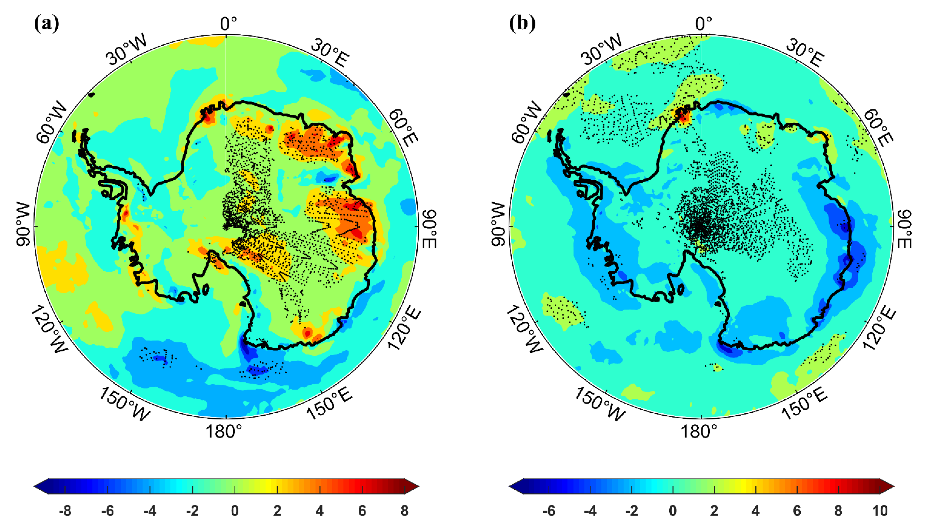
According to the variation trend of wind power density, the annually increasing areas are mainly distributed in Enderby—Queen Maude Land and near the Davis Station, while the decreasing areas are mainly distributed in Cape Adare and Mac.Robertson Land, followed by the Weddell Sea and the Ross Sea (−0.5~−1 W × m⁻² × a⁻¹). In spring, the land part shows a positive trend, and the vicinity of Cape Adair shows a negative trend. In summer, the positive trend decreases, and there is an area with a negative trend. The Southern Ocean shows an increasing trend. There is a negative trend in autumn and no significant change in winter.

(2)

According to the variation trend of EWSO, the increasing areas year by year are mainly distributed in the East Antarctic, while the decreasing areas are mainly distributed in the Ross Sea and Cape Adare. In spring, the East Antarctica and the Ross Ice Shelf show a positive trend, while the Ross Sea, Weddell Sea, and other waters show a decreasing trend. In summer, both strength and range of the trend decrease. In autumn and winter, only the Ross Sea and the Antarctic Peninsula show a decreasing trend, and the range of positive trends significantly reduces.

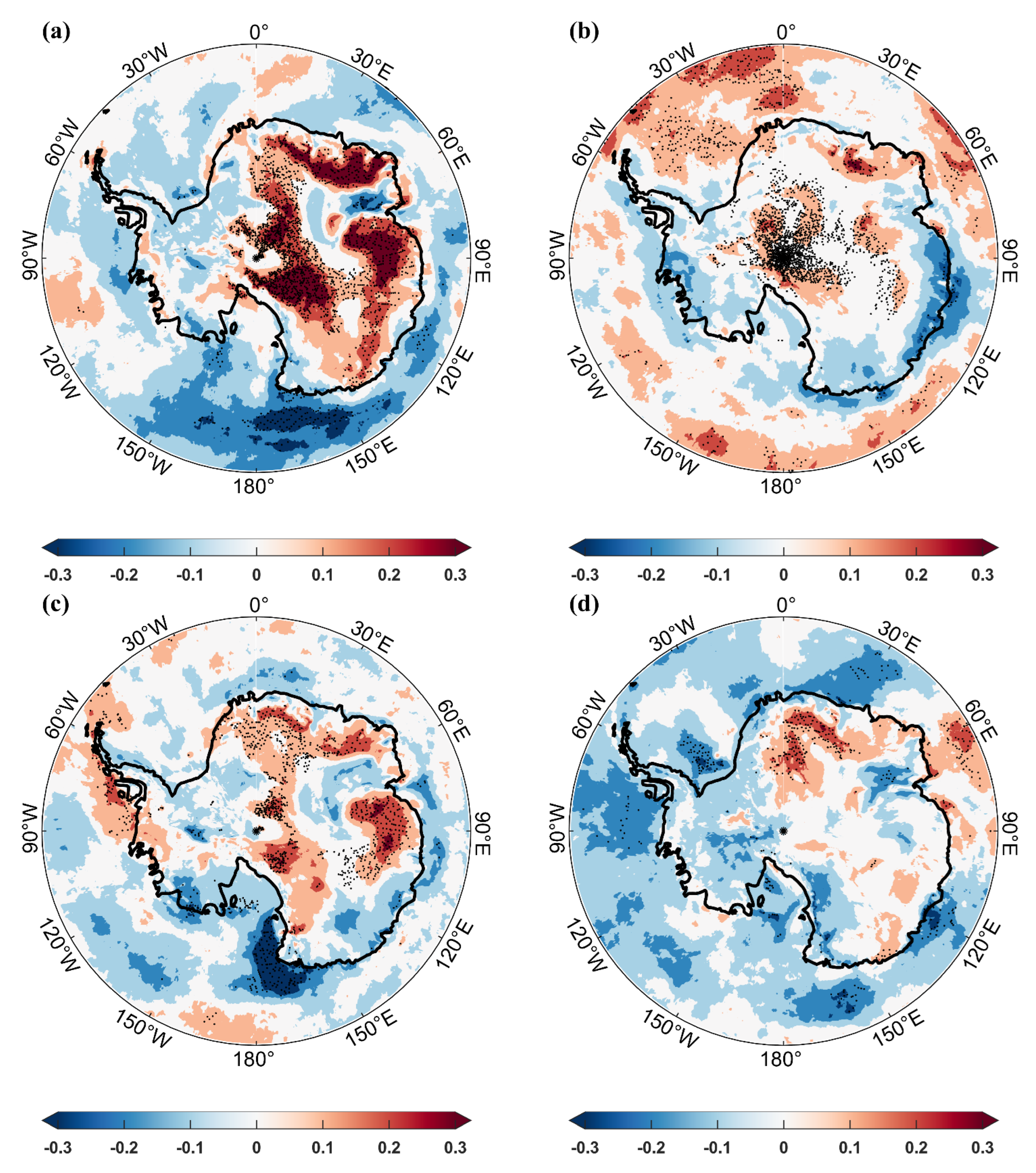
(3)

The variation trend of energy level occurrence, ALO: the seasonal and annual trend distribution of ALO is similar to that of EWSO, and its intensity is stronger than EWSO. RLO: except in summer, the range and intensity of ALO increase in other seasons, with positive trends in East Antarctica and negative trends in adjacent waters such as the Ross Sea. The biggest difference in summer is seen in the plains of East Antarctica, where ALO shows a significant positive trend while the trend of RLO remains unchanged. SLO: except in winter, the trend distribution of SLO and ALO changes greatly. The evolution trend of them in winter is basically the same, indicating that wind energy is more stable in winter. The differences are reflected in the extent of the positive trend in East Antarctica, with centers of positive trends occurring on both sides of the Prince Charles Mountains in spring, while the positive trend widens near the Trans-Antarctic Mountains. Summer and autumn: the positive trend of SLO in East Antarctica is largely absent or presents to a lesser extent but appears in the Southern Ocean.

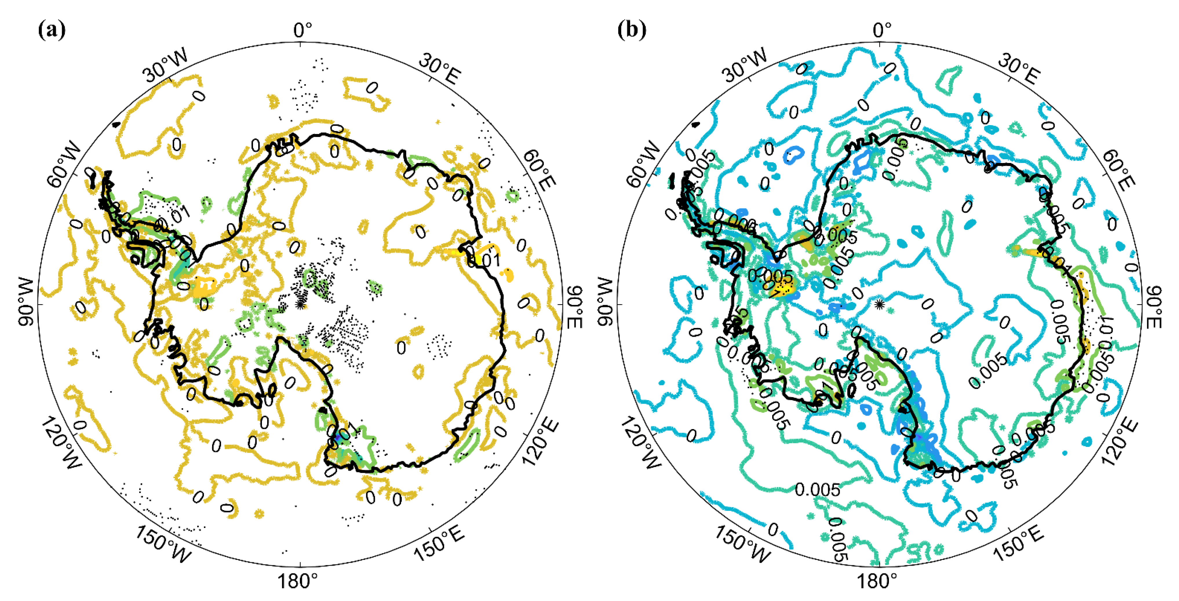
(4)

From the variation trend of wind energy stability, the increasing areas are mainly distributed on the coast of Queen Maude Land, the coast of West Antarctica, near the Ross Sea, the Trans-Antarctic Mountains; the Ronny Ice Shelf owns a decreasing trend, indicating that the stability becomes better. The trend in most of the rest of the region remains static, and it is consistent in different seasons. Monthly variation index: the areas with a significantly increasing trend are mainly distributed in the Prydz Bay, while the areas with a significantly increasing trend are mainly distributed in the West Antarctic—Antarctic Peninsula and Weddell Sea coast. Seasonal variation index: positive trends are distributed along the coast of Antarctica, the Ronny Ice Shelf, and the Weddell Sea-Southern Ocean, and negative trends are distributed along the Trans-Antarctic Mountains.

In conclusion, the East Antarctic coast of the Antarctic region, Wilhelm II Land-Wilkes Land, the South Pole—Kunlun station, and westerlies are superior in wind power density, effective wind speed occurrence, energy level occurrence, and stability variation trend, with a relatively large wind energy potential. Meanwhile, the coefficient of variation and monthly and seasonal variation index are superior near the South Pole, the Trans-Antarctic Mountains, the Weddell Sea, and the Ross Sea coast, but the variation trend of wind power density, availability, energy level frequency, and other indicators is significantly decreasing, with a relatively small wind energy potential.

The main shortcoming of using the ERA5 dataset for high latitude analysis is due to spatial resolution issues, which do not allow for a refined analysis of specific wind energy at locations or sites and only capture wind energy systematically. The inappropriate selection of the time resolution could result in missing sudden strong wind events or wind energy anomalies that occur at specific moments, which leads to inadequate analysis of wind energy utilization stability. Additionally, satellite data tends to be erroneous in high-latitude regions, which requires further data verification. This study focuses on long-term seasonal and annual averages and requires further research on whether sudden strong wind events or short periods are helpful for wind energy development. Least squares, along with linear regression, are used in this study, which may not be appropriate for certain periodic regions. Despite these flaws, this paper examines the evolution trend of Antarctic wind energy by using various key indicators. These findings provide a scientific basis for the construction and scientific research of Antarctic stations.

References

1. Jiang, S.; Hu, H.; Perrie, W.; Zhang, N.; Bai, H.; Zhao, Y. Different climatic effects of the Arctic and Antarctic ice covers on land surface temperature in the Northern Hemisphere: Application of Liang-Kleeman information flow method and CAM4.0. Clim. Dyn. 2022, 58, 1237–1255. [Google Scholar] [CrossRef]
2. Simmonds, I.; Jacka, T. Relationships between the Interannual Variability of Antarctic Sea Ice and the Southern Oscillation. J. Clim. 1995, 8, 637–648. [Google Scholar] [CrossRef]
3. Kolstad, E.; Bracegirdle, T. Marine cold-air outbreaks in the future: An assessment of IPCC AR4 model results for the Northern Hemisphere. Clim. Dyn. 2008, 30, 871–885. [Google Scholar] [CrossRef]
4. Liu, J.; Curry, J.; Martinson, D. Interpretation of recent Antarctic sea ice variability. Geophys. Res. Lett. 2004, 31, 2205. [Google Scholar] [CrossRef]
5. Shokr, M.; Ye, Y. Why Does Arctic Sea Ice Respond More Evidently than Antarctic Sea Ice to Climate Change? Ocean.-Land-Atmos. Res. 2023, 2, 0006. [Google Scholar] [CrossRef]
6. Yu, L.; Zhong, S. Strong Wind Speed Events over Antarctica and Its Surrounding Oceans. J. Clim. 2019, 32, 3451–3470. [Google Scholar] [CrossRef]
7. Qin, D.; Zhou, B.; Xiao, C. Progress in studies of cryospheric changes and their impacts on climate of China. J. Meteorol. Res. 2014, 28, 732–746. [Google Scholar] [CrossRef]
8. Fu, C. A possible relationship between pulsation of plum rains in chang-jiang valley and snow and ice cover on antarctica and the southern ocean. Chin. Sci. Bull. 1982, 1, 71–75. [Google Scholar]
9. Xue, F.; Guo, P.; Yu, Z. Influence of Interannual Variability of Antarctic Sea-Ice on Summer Rainfall in Eastern China. Adv. Atmos. Sci. 2003, 20, 97–102. [Google Scholar] [CrossRef]
10. Ma Lijuan, L.L. Relationship between Antarctic sea ice and the climate in summer of China. Chin. J. Polar Sci. 1956, 17, 1. [Google Scholar]
11. Cai, R. Effects of warming on soil carbon dioxide, methane emissions and generation mechanism in Antarctic. Master’s Thesis, East China Normal University, Shanghai, China, 2022. [Google Scholar] [CrossRef]
12. Khan, K.S.; Tariq, M. Wind resource assessment using SODAR and meteorological mast—A case study of Pakistan. Renew. Sustain. Energy Rev. 2018, 81, 2443–2449. [Google Scholar] [CrossRef]
13. Saulat, H.; Khan, M.M.; Aslam, M.; Chawla, M.; Rafiq, S.; Zafar, F.; Khan, M.M.; Bokhari, A.; Jamil, F.; Bhutto, A.W.; et al. Wind speed pattern data and wind energy potential in Pakistan: Current status, challenging platforms and innovative prospects. Environ. Sci. Pollut. Res. 2021, 28, 34051–34073. [Google Scholar] [CrossRef] [PubMed]
14. Gao, C.C.; Zheng, C.W.; Chen, X. Long-term trend analysis of wind energy resource in the China Sea and adjacent waters based on the CCMP wind data. Mar. Forecast. 2017, 34, 27–35. [Google Scholar]
15. Onea, F.; Rusu, L. A Study on the Wind Energy Potential in the Romanian Coastal Environment. J. Mar. Sci. Eng. 2019, 7, 142. [Google Scholar] [CrossRef]
16. Rusu, E. A 30-year projection of the future wind energy resources in the coastal environment of the Black Sea. Renew. Energy 2019, 139, 228–234. [Google Scholar] [CrossRef]
17. Lima, D.C.A.; Soares, P.M.M.; Cardoso, R.M.; Semedo, A.; Cabos, W.; Sein, D.V. The present and future offshore wind resource in the Southwestern African region. Clim. Dyn. 2021, 56, 1371–1388. [Google Scholar] [CrossRef]
18. Spezakis, Z.; Xydis, G. Transporting offshore wind power in the Western Gulf of Mexico: Retrofitting existing assets for power transmission via green hydrogen—A review. Environ. Sci. Pollut. Res. 2022, 1–12. [Google Scholar] [CrossRef]
19. Carreno-Madinabeitia, S.; Ibarra-Berastegi, G.; Sáenz, J.; Ulazia, A. Long-term changes in offshore wind power density and wind turbine capacity factor in the Iberian Peninsula (1900–2010). Energy 2021, 226, 120364. [Google Scholar] [CrossRef]
20. Wen, Y.; Kamranzad, B.; Lin, P. Assessment of long-term offshore wind energy potential in the south and southeast coasts of China based on a 55-year dataset. Energy 2021, 224, 120225. [Google Scholar] [CrossRef]
21. Costoya, X.; de Castro, M.; Carvalho, D.; Feng, Z.; Gómez-Gesteira, M. Climate change impacts on the future offshore wind energy resource in China. Renew. Energy 2021, 175, 731–747. [Google Scholar] [CrossRef]
22. Decastro, M.; Salvador, S.; Gómez-Gesteira, M.; Costoya, X.; Carvalho, D.; Sanz-Larruga, F.; Gimeno, L. Gimeno Europe, China and the United States: Three different approaches to the development of offshore wind energy. Renew. Sustain. Energy Rev. 2019, 109, 55–70. [Google Scholar] [CrossRef]
23. Carvalho, D.; Rocha, A.; Costoya, X.; Decastro, M.; Gómez-Gesteira, M. Wind energy resource over Europe under CMIP6 future climate projections: What changes from CMIP5 to CMIP6. Renew. Sustain. Energy Rev. 2021, 151, 111594. [Google Scholar] [CrossRef]
24. Xydis, G. A wind resource assessment around large mountain masses: The speed-up effect. Int. J. Green Energy 2015, 13, 616–623. [Google Scholar] [CrossRef]
25. Zheng, C.; Li, X.; Azorin-Molina, C.; Li, C.; Wang, Q.; Xiao, Z.; Yang, S.; Chen, X.; Zhan, C. Global trends in oceanic wind speed, wind-sea, swell, and mixed wave heights. Appl. Energy 2022, 321, 119327. [Google Scholar] [CrossRef]
26. Yu, L.; Zhong, S.; Sun, B. The Climatology and Trend of Surface Wind Speed over Antarctica and the Southern Ocean and the Implication to Wind Energy Application. Atmosphere 2020, 11, 108. [Google Scholar] [CrossRef]
27. Pourrahmani, H.; Zahedi, R.; Daneshgar, S.; Van herle, J. Lab-Scale Investigation of the Integrated Backup/Storage System for Wind Turbines Using Alkaline Electrolyzer. Energies 2023, 16, 3761. [Google Scholar] [CrossRef]
28. Zahedi, R.; Ahmadi, A.; Eskandarpanah, R.; Akbari, M. Evaluation of Resources and Potential Measurement of Wind Energy to Determine the Spatial Priorities for the Construction of Wind-Driven Power Plants in Damghan City. Int. J. Environ. Sustain. Dev. 2022, 11, 1–22. [Google Scholar] [CrossRef]
29. Zahedi, R.; Ghorbani, M.; Daneshgar, S.; Gitifar, S.; Qezelbigloo, S. Potential measurement of Iran’s western regional wind energy using GIS. J. Clean. Prod. 2022, 330, 129883. [Google Scholar] [CrossRef]
30. Zahedi, R.; Ahmadi, A.; Sadeh, M. Investigation of the load management and environmental impact of the hybrid cogeneration of the wind power plant and fuel cell. Energy Rep. 2021, 7, 2930–2939. [Google Scholar] [CrossRef]
31. Adem, A.; Halid, J.; Eugen, R. Temporal Variation of the Wave Energy Flux in Hotspot Areas of the Black Sea. Sustainability 2019, 11, 562. [Google Scholar] [CrossRef]
32. Bahareh, K.; Kaoru, T. A climate-dependent sustainability index for wave energy resources in Northeast Asia. Energy 2020, 209, 118466. [Google Scholar] [CrossRef]
33. Danial, K.; Seyed, M.M.; William, G.; Gregorio, I. Wave energy status in Asia. Ocean Eng. 2018, 169, 344–358. [Google Scholar] [CrossRef]
34. Sreelakshmi, S.; Bhaskaran, P.K. Spatio-Temporal Distribution and Variability of High Threshold Wind Speed and Significant Wave Height for the Indian Ocean. Pure Appl. Geophys. 2020, 177, 4559–4575. [Google Scholar] [CrossRef]
35. Soares, P.M.M.; Lima, D.C.A.; Nogueira, M. Global offshore wind energy resources using the new ERA-5 reanalysis. Environ. Res. Lett. 2020, 15, 1040a2. [Google Scholar] [CrossRef]
36. Beck, H.E.; Pan, M.; Roy, T.; Weedon, G.P.; Pappenberger, F.; van Dijk, A.I.J.M.; Huffman, G.J.; Adler, R.F.; Wood, E.F. Daily evaluation of 26 precipitation datasets using Stage-IV gauge-radar data for the CONUS. Hydrol. Earth Syst. Sci. 2019, 23, 207–224. [Google Scholar] [CrossRef]
37. Nogueira, M. Inter-comparison of ERA-5, ERA-interim and GPCP rainfall over the last 40 years: Process-based analysis of systematic and random differences. J. Hydrol. 2020, 583, 124632. [Google Scholar] [CrossRef]
38. Johannsen, F.; Ermida, S.; Martins, J.P.A.; Trigo, I.F.; Nogueira, M.; Dutra, E. Cold Bias of ERA5 Summertime Daily Maximum Land Surface Temperature over Iberian Peninsula. Remote Sens. 2019, 11, 2570. [Google Scholar] [CrossRef]
39. Urraca, R.; Huld, T.; Gracia-Amillo, A.; Martinez-de-Pison, F.J.; Kaspar, F.; Sanz-Garcia, A. Evaluation of global horizontal irradiance estimates from ERA5 and COSMO-REA6 reanalyses using ground and satellite-based data. Sol. Energy 2018, 164, 339–354. [Google Scholar] [CrossRef]
40. Zheng, C.; Li, X.; Luo, X.; Chen, X.; Qian, Y.; Zhang, Z.; Gao, Z.; Du, Z.; Gao, Y.; Chen, Y. Projection of Future Global Offshore Wind Energy Resources using CMIP Data. Atmosphere-Ocean 2019, 57, 134–148. [Google Scholar] [CrossRef]
41. Zheng, C.W. Temporal-spatial characteristics dataset of offshore wind energy resource for the 21st Century Maritime Silk Road. China Sci. Data 2020, 5, 106–119. [Google Scholar]
42. Kodama, Y.; Wendler, G. Wind and temperature regime along the slope of Adelie Land, Antarctica. J. Geophys. Res. Atmos. 1986, 91, 6735–6741. [Google Scholar] [CrossRef]
43. Parish, T.R. Surface Airflow Over East Antarctica. Mon. Weather. Rev. 1982, 110, 84–90. [Google Scholar] [CrossRef]
44. Parish, T.R.; Bromwich, D.H. The Inversion Wind Pattern over West Antarctica. Mon. Weather. Rev. 1986, 114, 849–860. [Google Scholar] [CrossRef]
Figure 1. The variation trend of wind power density in spring (a), summer (b), autumn (c), and winter (d) and its annual average (e) in the Antarctic region (unit: W × m−2 × a−1).
Jmse 11 01088 g001aJmse 11 01088 g001b
Figure 2. The variation trend of effective wind speed occurrence in spring (a), summer (b), autumn (c), and winter (d) and its annual average (e) in the Antarctic region (unit: %/a).
Jmse 11 01088 g002aJmse 11 01088 g002b
Figure 3. The variation trend of ALO in spring (a), summer (b), autumn (c), and winter (d) and its annual average (e) in the Antarctic region (unit: %/a).
Jmse 11 01088 g003aJmse 11 01088 g003b
Figure 4. The variation trend of RLO in spring (a), summer (b), autumn (c), and winter (d) and its annual average (e) in the Antarctic region (unit: %/a).
Jmse 11 01088 g004aJmse 11 01088 g004b
Figure 5. The variation trend of SLO of spring (a), summer (b), autumn (c), and winter (d) and its annual average (e) in the Antarctic region (unit: %/a).
Jmse 11 01088 g005aJmse 11 01088 g005b
Figure 6. The variation trend of Cv in spring (a), summer (b), autumn (c), and winter (d) and its annual average (e) in the Antarctic region (unit: a−1).
Jmse 11 01088 g006aJmse 11 01088 g006b
Figure 7. The variation trend of Mv (a) and Sv (b) in the Antarctic region (unit: a−1).
Jmse 11 01088 g007
Disclaimer/Publisher’s Note: The statements, opinions and data contained in all publications are solely those of the individual author(s) and contributor(s) and not of MDPI and/or the editor(s). MDPI and/or the editor(s) disclaim responsibility for any injury to people or property resulting from any ideas, methods, instructions or products referred to in the content.