A Curvelet-Transform-Based Image Fusion Method Incorporating Side-Scan Sonar Image Features

Abstract

Current methods of fusing side-scan sonar images fail to tackle the issues of shadow removal, preservation of information from adjacent strip images, and maintenance of image clarity and contrast. To address these deficiencies, a novel curvelet-transform-based approach that integrates the complementary attribute of details from side-scan sonar strip images is proposed. By capitalizing on the multiple scales and orientations of the curvelet transform and its intricate hierarchical nature, myriad fusion rules were applied at the corresponding frequency levels, enabling a more-tailored image fusion technique for side-scan sonar imagery. The experimental results validated the effectiveness of this method in preserving valuable information from side-scan sonar images, reducing the presence of shadows and ensuring both clarity and contrast in the fused images. By meeting the aforementioned challenges encountered in existing methodologies, this approach demonstrated great practical significance.

1. Introduction

Side-scan sonar imagery represents the primary wellspring of information for unveiling seafloor topography and discerning underwater navigational obstructions. The prevailing method for side-scan sonar measurements is underwater towed exploration, which generates images with the following features. Firstly, the positional accuracy of targets in side-scan sonar imagery is compromised by imprecise towing locations. Secondly, adjacent strips exhibit complementary details of the same seafloor targets. Thirdly, shadows formed by measuring strips of different orientations cannot be expressed in a fused manner, as their length in sonar images reflects the height of the targets. Lastly, the capricious interplay of intricate marine ambient noise and vessel orientation engenders volatility in image fidelity. Side-scan sonar image fusion is designed to process side-scan sonar multiple-strip images in accordance with specific rules and methodologies. While leveraging the complementary information between overlapping strip images and preserving the maximum valuable content from strips, the technique maintains the contrast and clarity of fused imagery, thereby bolstering precision in image interpretation and target identification [1].

Typically, side-scan sonar image fusion is performed in the spatial domain or transform domain, these two types of methods indeed being interconnected; however, they exhibit fundamental differences in terms of their underlying concepts and principles. The spatial domain image fusion technique involves weighted averaging of the pixel values of the corresponding positions in the overlapping regions of adjacent strips to generate a new image. Though user-friendly and computationally efficient, the approach falls short in preserving fine details in side-scan sonar imagery, as it tends to underplay valuable details and underscore those that are irrelevant [2,3,4,5,6]. In the spatial domain method, the multiband image fusion method, however, offers a greater potential for improving fusion outcomes. It involves decomposing side-scan sonar images into Gaussian or Laplacian pyramids and fusing the corresponding images at different resolutions before reconstructing the fused pyramid into a new fused image [7]. Inspired by optical image fusion, the approach takes no account of integrating the features of side-scan sonar imagery, thus lacking specific mechanisms for removing shadows and preserving details [2,3,4]. The transform domain image fusion technique enables analysis followed by a conversion of side-scan sonar images from the spatial domain to other domains. For instance, image fusion based on the wavelet transform [6,8,9,10] decomposes wavelets of adjacent strip images into multilevel frequency domain coefficients and fuses these coefficients, which are then inversely transformed into the new side-scan sonar mosaic image. An examination of images from the perspective of the frequency domain suggests that the method mitigates the limitations of spatial domain analysis in capturing critical information. Despite its exceptional processing of one-dimensional linear signals, the wavelet-transform-based approach falls short of comprehensively profiling two-dimensional side-scan sonar imagery [2,3,4,5,6,11] as it cannot achieve “information integration, shadow removal, and high clarity and contrast.” In transform domain methods, image fusion built on the multiscale geometric transform analyzes side-scan sonar images using waveforms with multiple scales and of various orientations, which complements wavelet-transform-based methods on the orientational front. The transform domain image fusion approaches are often coupled with feature extraction algorithms. For instance, the Canny operator can extract edge contours from the high-frequency components obtained upon wavelet decomposition, prioritizing edge information during fusion and recombination [12]. The wavelet transform can be blended with weighted averaging to process wavelet coefficients [8,13,14]. Imagery can be divided into high-frequency and low-frequency components for processing using pyramid methods and wavelet transform, respectively [15]. Some researchers performed curvelet decomposition on images, followed by edge information extraction using edge detection operators. While overcoming the limitations of the wavelet transform, the curvelet transform also addresses the inadequacy of edge detection operators under multiscale analysis [16]. Despite that, current side-scan sonar image fusion techniques expanding on the curvelet transform still deliver suboptimal fusion outcomes as they fail to take full account of the features of side-scan sonar imagery [17].

On that basis, we propose a curvelet-transform-based, hierarchical image fusion technique that integrates such features of side-scan sonar strip image information as complementary. Featuring the curvelet transform’s anisotropy and intricate frequency bands, the approach involves the application of various rules governing the features of side-scan sonar imagery to different frequency bands. This way, the fused image can fully exhibit the valuable details of both images and remove shadows while guaranteeing higher image clarity and contrast.

2. Process of the Curvelet-Transform-Based Side-Scan Sonar Image Fusion Algorithm

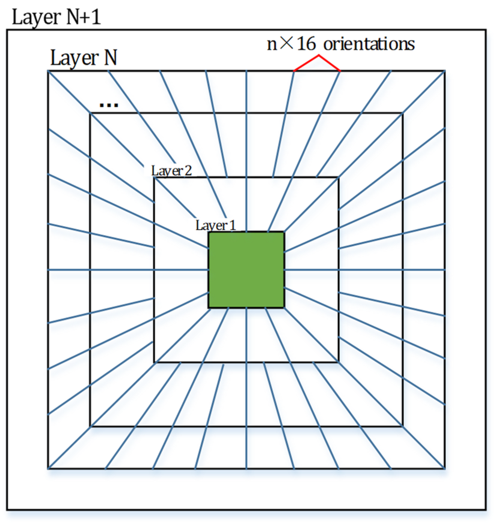
2.1. Curvelet-Transform-Based Algorithm

In processing two-dimensional imagery under the classic wavelet transform, the two-dimensional wavelet basis formed by the tensor product of one-dimensional wavelets can only respond to feature information at limited orientations. The curvelet transform, in contrast, addresses the issue as it is capable of showing a response to such information at various orientations on a plane. The equation of the continuous curvelet transform is expressed as follows [16]:

$$\mathrm{C}(k,\theta ,x,y)=<I,{{\displaystyle \varphi }}_{k,\theta ,x,y}(a,b)>={\displaystyle \iint I(a,b)•{{\displaystyle \varphi }}_{k,\theta ,x,y}(a,b)dadb}$$

(1)

where $\mathrm{C}$ is the curvelet coefficient; $k$ denotes the curvelet’s scale; $\theta$ indicates the curvelet’s orientation; $x,y$ suggest the curvelet coefficient’s location; $I(a,b)$ is the input image; $(a,b)$ represents the pixel’s point location; $\varphi (a,b)$ indicates the curvelet function. As shown in Equation (1), curvelets are parameterized by scale, orientation, and location. They showcase the vector information of point features in a straightforward manner, as displayed in Figure 1.

As a continuous transformation theory, the curvelet transform theoretically sees seamless and constant changes in scale and orientation. However, infinite scale changes are impractical. As such, it is necessary to render the continuous curvelet transform discrete and finite.

The discrete curvelet transform is mathematically expressed as:

$$\mathrm{C}(k,\theta ,x,y)={\displaystyle \sum _{a=0}^{A-1}{\displaystyle \sum _{b=0}^{B-1}I(a,b)•{{\displaystyle \varphi }}_{k,\theta ,x,y}(a,b)}}$$

(2)

where $A\times B$ represents the image size.

In light of the abovementioned theory, the discrete curvelet transform’s frequency domain, as shown in Figure 2, features an image decomposed into multiple layers of coefficients, with each layer comprising curvelets of various orientations and at different scales.

In a discretized model, the number of layers depends on the size of an image, with a greater image size engendering more layers. Except for the first and last layers, which are characterized by a single orientation, each of the remaining layers has $16\times n$ orientations, with n irrelevant to N, the layer number. In addition, each orientation contains the corresponding curvelet coefficient and information about its location. The first layer, known as the coarse layer, represents the coarse low-frequency information of the image. The size of the coefficient matrix in this layer is contingent upon the scale of the curvelet function. The intermediate layers, collectively referred to as the detail layers, capture the medium- to high-frequency details. The coefficient matrix’s size in these layers is determined by both the scale and orientation of the curvelet function. The last or utmost layer, called the fine layer, epitomizes the intricate details within the high-frequency spectrum. In this layer, the dimensions of the coefficient matrix correspond precisely to the image size [17], as presented in

Table 1. The hierarchical structure of coefficients in the curvelet transform.

Layer	Scale Coefficient	Number of Orientations	Matrix Form
Coarse	$C\left\{1\right\}$	1	A set of matrices
Detail	$C\left\{2\right\}$	16	16 sets of matrices
	…	…	…
	$C\left\{N\right\}$	$16\times n$ (with n irrelevant to N)	$16\times n$ sets of matrices
Fine	$C\{N+1\}$	1	A set of matrices of size $A\times B$

.

2.2. Fusion Process

The algorithmic procedure for fusing side-scan sonar images under the curvelet transform is as follows:

Step 1: Perform curvelet decomposition on the overlapping portions of two side-scan sonar strip images separately, and obtain curvelet coefficients;

Step 2: Adopt diverse selection and fusion rules (see Figure 3) to generate the fused curvelet coefficients;

Step 3: Implement the inverse curvelet transform on the fused curvelet coefficients to produce the fused side-scan sonar image.

Rules for fusing curvelet coefficients at different layers were formulated by factoring in the features of side-scan sonar images.

3. Rules for Fusion of Curvelet Coefficients

3.1. Fusion Rules at the Coarse Layer

In side-scan sonar imagery, the height of detected targets is generally represented by the shadow length, but such information is deemed irrelevant during the image fusion process. Considering that shadows in side-scan sonar strip images typically exhibit low reflection intensity, these regions, upon the curvelet transform, would yield greater absolute values of the low-frequency coefficients. Therefore, to mitigate the impact of shadows on the fused side-scan sonar image [9], the curvelet coefficient at the coarse layer was selected by retaining the coefficient with the smallest absolute value. The computational equation is:

$$\{\begin{array}{c}C(x,y)=C_1(x,y),(\left|C_1(x,y)\right|<\left|C_2(x,y)\right|)\\ C(x,y)=C_2(x,y),(\left|C_1(x,y)\right|>\left|C_2(x,y)\right|)\end{array}$$

(3)

where $C(x,y)$ is the fused coefficient; $C_1(x,y)$ and $C_2(x,y)$ represent the coefficients to be fused.

3.2. Fusion Rules at the Detail Layers

The process of side-scan sonar image fusion necessitates the use of complementary information from adjacent strips [6]. The overlapping parts of side-scan sonar strip images contain both redundant and complementary details. While redundant data can be partially retained, those complementary details need to be equally preserved. Hence, the selection of fusion rules at the detail layer is expanded by a fusion algorithm based on the regional matching degree. This algorithm calculates the extent to which the intermediate-frequency curvelet coefficients of two images within the same region match, thereby distinguishing between redundant and complementary information. When calculating the matching degree, it is optimal to choose the $7\times 7$ window size [18,19], which effectively represents the gray-level characteristics in the region. A small window size may reduce the amount of information, rendering the matching degree calculation useless. Conversely, a large window size is likely to cause an imbalanced distribution algorithm, as there would emerge an overwhelming number of regions with low matching degrees given the excessive irrelevant details produced. The equation for calculating the matching degree is as follows:

$$M=\frac{\frac{2}{49}{\displaystyle \sum _{i,j=-1}^{5}w(1+i,1+j)\times (C_1(x+i,y+j)\times }{C}_2(x+i,y+j))}{E_1+E_2}$$

(4)

$$E_1=\frac{1}{49}{\displaystyle \sum _{i,j=-1}^{5}w(1+i,1+j)\times C_1{(x+i,y+j)}^2}$$

(5)

$$E_2=\frac{1}{49}{\displaystyle \sum _{i,j=-1}^{5}w(1+i,1+j)\times C_2{(x+i,y+j)}^2}$$

(6)

$$w=\frac{1}{484}{w}_1^T\times w_1$$

(7)

where $M$ is the matching degree; $E$ denotes the regional activity degree [18]; $w$ represents the weighting coefficient matrix; $w_1=[1,2,4,8,4,2,1]$.

The matching degree is determined by a set threshold value, which decides whether the information is redundant or complementary. An empirical threshold value of 0.7 is preferred, as employing other values would engender imbalances in the distribution rules. The threshold was determined by testing nine threshold values ranging from 0.1 to 0.9 on two types of side-scan sonar images, namely “side-scan sonar images with strong noise” and “side-scan sonar images with larger shadow areas”. The threshold value of 0.7 exhibited the best visual effect and performance evaluation among all the tested values. A threshold greater than 0.7 comes with a higher matching degree, which leaves most coefficients ineffective and valuable information elusive. This is also known as the “Type I Error” or a “false positive” finding. On the other hand, when the threshold is lower than 0.7, a large amount of low-value information is included in the weighted averaging, thus leading to the “Type II Error” or a “false negative” conclusion. Both of these “errors” contribute to a decrease in the fidelity evaluation of the fused image.

The matching degree exceeding the threshold indicates that the part of that region is redundant. In this case, a fade-in and fade-out weighted averaging algorithm should be employed to increase the weighting coefficients for low-activity regions and relate these coefficients to the matching degree value. Higher matching degrees correspond to a larger proportion of low-energy coefficients, making the fused coefficient closer to the low-activity coefficient value. This approach is designed to minimize the error caused by the distortion of side-scan sonar images while preserving information of high similarity. The equations for the fade-in and fade-out weighted averaging are expressed as follows:

$$\{\begin{array}{c}C(x,y)=\frac{1}{2}\{(1-\frac{1-M}{1-0.7})C_1(x,y)+(1+\frac{1-M}{1-0.7})C_2(x,y)\},(E_1>E_2)\\ C(x,y)=\frac{1}{2}\{(1+\frac{1-M}{1-0.7})C_1(x,y)+(1-\frac{1-M}{1-0.7})C_2(x,y)\},(E_1<E_2)\end{array}$$

(8)

When the matching degree falls below or equals the threshold value, it signifies the presence of the complementary region, where one image exhibits shadowed areas, while the other contains valid information. In such instances, the coefficients with elevated activity within the region are selectively retained [18] to preserve the complementary details from both strip images. The algorithmic equations for this procedure are:

$$\{\begin{array}{c}C(x,y)=C_1(x,y),(E_1>E_2)\\ C(x,y)=C_2(x,y),(E_1<E_2)\end{array}$$

(9)

To guarantee the smoothness of image information and avoid outliers, the central point coefficient served as the coefficient during the selection and fusion processes.

3.3. Fusion Rules at the Fine Layer

Beyond the intricate target features of side-scan sonar images, high-frequency coefficients contain significant amounts of noise, which remain even upon pre-processing and denoising. That means a technique equivalent to enhancement or sharpening should be applied to coefficients at the fine layer, ensuring that the fused side-scan sonar image exhibits contrast and clarity equal to or greater than the individual strip images. To meet these requirements, parameters that reflect contrast and clarity must be considered. Commonly used ones are the average gray-level gradient [7,18] and the regional gray-level variance [8,19]. The preferred approach is an extremum selection algorithm based on the average gray-level gradient. Under the algorithm, the extreme value, upon the calculation of the average gradient, is retained, a technique similar to enhancement or sharpening, which ensures the fused side-scan sonar image possesses contrast and clarity that are not inferior to the individual strip images. The distinctive feature of this algorithm is that higher average gradient values correspond to a stronger contrast of the coefficients in the region and clearer target features in the side-scan sonar image. By contrast, lower average gradient values indicate weaker contrast and blurrier target features. The equation for calculating the average gray-level gradient is expressed as:

$$S=\frac{1}{m\times n}{\displaystyle \sum _{i=0}^{m-1}{\displaystyle \sum _{j=0}^{n-1}\sqrt{\frac{1}{2}\times \left[{\left(\frac{\partial C(x,y)}{\partial x}\right)}_{(i,j)}^2+{\left(\frac{\partial C(x,y)}{\partial y}\right)}_{(i,j)}^2\right]}}}$$

(10)

where $S$ is the average gray-level gradient; $m\times n$ denotes the size of the matrix of gray-level gradient values, the same as that of the curvelet coefficients. The coefficient fusion equations under this algorithm are:

$$\{\begin{array}{c}C(x,y)=C_1(x,y),(S_1>S_2)\\ C(x,y)=C_2(x,y),(S_1<S_2)\end{array}$$

(11)

4. Evaluation Indicators

The indicators typically employed to assess the effectiveness of side-scan sonar image fusion include information entropy, normalized mutual information, average gradient, spatial frequency, and standard deviation:

(1)

Information entropy:

Information entropy can be used to quantify the information value of the fused side-scan sonar image. A higher numerical value indicates more uncertainty and greater information value of the fused image, thus suggesting higher image fidelity [2,3,6,8,11,18,19,20,21,22,23].

$$H(x)=-{\displaystyle \sum _{i=1}^L{h}_x(i){\log }_2}{h}_x(i)$$

(12)

In Equation (12), $L$ is the gray level of an image; $H(x)$ represents the information entropy; $h_x(i)$ denotes the probability distribution of the gray level of the image pixels.

(2)

Normalized mutual information:

The fusion of side-scan sonar images using normalized mutual information preserves the information proportionality of strip imagery, whereby a higher ratio value signifies a greater extent of information preservation and superior fidelity [2,21,23]. Nonetheless, this indicator tends to allow for distortion and errors pertaining to underwater features and seafloor topography. With matching and correction in the early stages, error information can be diminished to render the indicator more effective and reliable.

$$MNI(x,y;f)=\frac{NMI(x,f)+NMI(y,f)}{2}$$

(13)

$$NI(x,f)=\frac{I(x,f)}{(H(x)+H(f))/2}$$

(14)

$$I(x,f)=H(x)+H(f)-H(x,f)={\displaystyle \sum _{i=1}^L{\displaystyle \sum _{j=1}^L{h}_{x,f}(i,j){\log }_2\frac{h_{x,f}(i,j)}{h_x(i)h_f(j)}}}$$

(15)

$$H(x,f)=-{\displaystyle \sum _{i=1}^L{\displaystyle \sum _{j=1}^L{h}_{x,f}(i,j){\log }_2}}{h}_{x,f}(i,j)$$

(16)

In the above equations, $x$ and $y$ represent the location of the pixel of a pre-mosaic strip image; $f$ is the mosaic image; $h_{x,f}(i,j)$ denotes the joint probability distribution of $x$ and $f$; $H(x,f)$ indicates the joint entropy.

(3)

Average gradient:

The average gradient is a measure of image clarity and contrast, which is also applicable to the fused side-scan sonar image, with a higher value leading to a clearer and higher-fidelity fused image [8,19,20,21,22,23].

$$grad=\frac{1}{A\times B}{\displaystyle \sum _{a=1}^A{\displaystyle \sum _{b=1}^B\sqrt{\frac{1}{2}\times \left[{\left(\frac{\partial I}{\partial x}\right)}_{(a,b)}^2+{\left(\frac{\partial I}{\partial y}\right)}_{(a,b)}^2\right]}}}$$

(17)

where $A\times B$ is the image size; $I$ suggests the matrix of image pixel values; $\frac{\partial I}{\partial x}$ represents the partial derivative of the gradient; $(a,b)$ indicates where the pixel point or the partial derivative of the gradient is located.

(4)

Spatial frequency:

The spatial frequency describes how spatially active an image is, and as its numerical value goes up, the fidelity of the fused side-scan sonar image increases [3,18].

$$SF=\sqrt{C{F}^2+R{F}^2}$$

(18)

$$CF=\sqrt{\frac{1}{A\times B}{\displaystyle \sum _{a=2}^A{\displaystyle \sum _{b=1}^B{(I(a,b)-I(a-1,b))}^2}}}$$

(19)

$$RF=\sqrt{\frac{1}{A\times B}{\displaystyle \sum _{a=1}^A{\displaystyle \sum _{b=2}^B{(I(a,b)-I(a,b-1))}^2}}}$$

(20)

where $CF$ is the spatial column frequency; $RF$ denotes the spatial row frequency.

(5)

Standard deviation:

Indicative of gray-level value dispersion, the standard deviation also reflects the contrast of the fused side-scan sonar image, and a larger numerical standard deviation value is accompanied by a higher level of contrast, thus delivering fusion results of higher fidelity [2,3,6,8,11,20].

$$D=\sqrt{{\displaystyle \sum _{i=0}^{255}{(i-ave)}^{2}h(i)}}$$

(21)

In Equation (20), $i$ is the gray level, whose value ranges from 0 to 255; $ave$ denotes the average gray-level value of pixels in an image (or a selected box); $h(i)$ represents the probability distribution of pixels with gray level i.

5. Experiments and Analyses

The fidelity of side-scan sonar images is profoundly impacted by noise, which finds its expression in low noise and strong noise. Image shadows can be classified based on their area. For experimental purposes, we selected two representative types of images.

5.1. Testing on the Side-Scan Sonar Image with Low Noise and Large Shadow Areas

To analyze and compare the strengths and weaknesses of various fusion algorithms and validate the applicability of our proposed algorithm, we carefully handpicked a dataset from the SonarWiz side-scan sonar software website. The dataset, as depicted in Figure 4, was obtained on 12 May 2009, in the eastern coastal waters of New Hampshire, United States of America, using a Klein towed side-scan sonar system. The local water depth was approximately 30 m, and the instrument’s measurement range was set to a single-sided swath of 100 m. Notably, the dataset demonstrates low noise levels, expansive shadow areas, and distinct geomorphic features.

Taken from Figure 4, the cropped image apparently containing distinct geomorphic features was converted into a gray-level one before matching image feature points [10], with the matching results shown in Figure 5. To match the images, the specific method involved selecting the corresponding feature points of common targets in both images, using the left image as the reference, and moving the right image to align with the same feature points. Matching serves as a pre-work for fusion. The algorithm proposed in this paper was designed based on the accurate matching of image positions. Therefore, the matching method was not relevant to the fusion algorithm proposed in this paper.

Figure 6 illustrates the overlaid display of the positional relationship following the matching process. A region of overlapping coverage measuring 439 $\times$ 175 pixels was selected from the experimental image for the curvelet transform, with the hierarchical structure presented in

Table 2. The hierarchical structure of the experimental image upon the curvelet transform.

Layer	Scale Coefficient	Number of Orientations	Matrix Form
Coarse	$C\left\{1\right\}$	1	37 $\times$ 15
Detail	$C\left\{2\right\}$	16	30 $\times$ 16 (4 sets) 27 $\times$ 14 (4 sets) 37 $\times$ 13 (4 sets) 37 $\times$ 11 (4 sets)
	$C\left\{3\right\}$	32	58 $\times$ 16 (4 sets) 55 $\times$ 15 (8 sets) 55 $\times$ 16 (4 sets) 37 $\times$ 24 (4 sets) 38 $\times$ 22 (8 sets) 37 $\times$ 22 (4 sets)
	$C\left\{4\right\}$	32	115 $\times$ 30 (4 sets) 110 $\times$ 30 (12 sets) 74 $\times$ 46 (4 sets) 74 $\times$ 44 (12 sets)
Fine	$C\left\{5\right\}$	1	439 $\times$ 175

.

When the selected region was gradually reduced, the number of layers decreased from 5 to 4 and further to 3, which is the minimum number of layers. The number of orientations per layer was as follows: 1 and 16 (for 3 layers), 1 (for 4 layers), and 1. When the selected region was expanded, the number of layers increased from 5 to 6, 7, and so on, depending on the image size. In this case, the number of orientations per layer was as follows: 1, 16, 32, and 32 (for 5 layers), 64 (for 6 layers), 64 (for 7 layers) … and 1.

To demonstrate the effectiveness of the proposed method in this paper, a comparative analysis was conducted with such techniques as the curvelet-transform-based fusion method factoring in the extremum and the fade-in and fade-out weighted averaging rule, the wavelet-transform-based fusion method following this study’s rules, the Laplacian pyramid fusion method following this study’s rules, and the fade-in and fade-out fusion strategy based on the rules stated in this paper.

The images depicted in Figure 7 were all locally cropped and arranged from left to right as follows: ① left strip image; ② right strip image; ③ fused image using the proposed method; ④ image using the curvelet-transform-based fusion method incorporating the extremum and the averaging rule; ⑤ fused image upon the wavelet transform; ⑥ image adopting a three-layer Laplacian pyramid fusion approach; ⑦ image using a four-layer Laplacian pyramid fusion technique; ⑧ image employing a five-layer Laplacian pyramid fusion method; ⑨ image using the gray-level-based fade-in and fade-out weighted averaging fusion method. Data on the evaluation indicators are illustrated in

Table 3. Data on evaluation indicators for various image fusion methods.

		Normalized Mutual Information	Information Entropy	Average Gradient	Spatial Frequency	Standard Deviation of Gray Level of Image
Proposed Method		0.1433	7.6675	14.3056	37.6845	54.4358
Curvelet-Transform-Based Fusion Method Incorporating the Extremum and the Fade-In and Fade-Out Weighted Averaging Rule		0.0954	6.7515	11.9239	36.6779	38.5593
Fusion Method Based on the Wavelet Transform		0.1033	7.3513	13.6859	37.1228	41.2944
Laplacian Pyramid Fusion Method	Three Decomposed Layers	0.1205	7.5844	13.6903	37.1458	49.5006
	Four Decomposed Layers	0.1047	7.5831	13.5391	37.0545	48.4813
	Five Decomposed Layers	0.0881	7.4808	12.7595	33.1743	50.3156
Gray-Level-Based Fade-In and Fade-Out Weighted Averaging Fusion Method		0.0802	7.1200	8.4047	22.8736	34.8301

.

The analysis of Figure 7 shows that the wavelet-transform-based fusion method displayed a relatively diminished visual contrast. The curvelet-transform-enabled fusion technique incorporating the extremum and the fade-in and fade-out weighted averaging rule exhibited unsatisfactory performance in terms of both image clarity and contrast, even falling below the outcomes of its counterpart built on the wavelet transform. The Laplacian pyramid fusion method manifested the presence of white shadows, which obscured the valid information, and varying degrees of mottling. A decrease in the number of layers resulted in reduced shadowing, thereby minimizing information loss, but increasing the occurrence of mottling. By contrast, an increasing number of layers amplified shadowing while mitigating the emergence of mottling. Furthermore, the gray-level-based fade-in and fade-out weighted averaging fusion method incurred conspicuous information loss. In stark contrast, the proposed method in this paper delivered a markedly superior visual performance when compared to the aforementioned approaches.

As shown in the data of Table 3:

The evaluation ranking of Indicator 1 was: proposed method > Laplacian 3-layer pyramid fusion method > Laplacian 4-layer pyramid fusion method > fusion method based on the wavelet transform > curvelet-transform-based fusion method incorporating the extremum and the fade-in and fade-out weighted averaging rule > Laplacian 5-layer pyramid fusion method > gray-level-based fade-in and fade-out weighted averaging fusion method.

The evaluation ranking of Indicator 2 was: proposed method > Laplacian 3-layer pyramid fusion method > Laplacian 4-layer pyramid fusion method > Laplacian 5-layer pyramid fusion method > fusion method based on the wavelet transform > gray-level-based fade-in and fade-out weighted averaging fusion method > curvelet-transform-based fusion method incorporating the extremum and the fade-in and fade-out weighted averaging rule.

The evaluation ranking of Indicator 3 was: proposed method > Laplacian 3-layer pyramid fusion method > fusion method based on the wavelet transform > Laplacian 4-layer pyramid fusion method > Laplacian 5-layer pyramid fusion method > curvelet-transform-based fusion method incorporating the extremum and the fade-in and fade-out weighted averaging rule > gray-level-based fade-in and fade-out weighted averaging fusion method.

The evaluation ranking of Indicator 4 was: proposed method > Laplacian 3-layer pyramid fusion method > fusion method based on the wavelet transform > Laplacian 4-layer pyramid fusion method > curvelet-transform-based fusion method incorporating the extremum and the fade-in and fade-out weighted averaging rule > Laplacian 5-layer pyramid fusion method > gray-level-based fade-in and fade-out weighted averaging fusion method.

The evaluation ranking of Indicator 5 was: proposed method > Laplacian 5-layer pyramid fusion method > Laplacian 3-layer pyramid fusion method > Laplacian 4-layer pyramid fusion method > fusion method based on the wavelet transform > curvelet-transform-based fusion method incorporating the extremum and the fade-in and fade-out weighted averaging rule > gray-level-based fade-in and fade-out weighted averaging fusion method.

The indicator data provided in Table 3 confirmed that, by incorporating the rules proposed in this study, the curvelet-transform-based image fusion method outperformed the approach of incorporating the extremum and the averaging rule. Therefore, with optimal indicator performance among other fusion methods, the proposed technique that integrates the rules on fusing the features of side-scan sonar images with curvelet decomposition demonstrated a strong applicability to side-scan sonar images with low noise and large shadow areas.

5.2. Testing on the Side-Scan Sonar Image with Strong Noise and Small Shadow Areas

Utilizing an AUV to collect side-scan sonar images is a valuable research method, and several studies in the industry are currently based on this approach [24,25,26]. The image depicted in Figure 8 illustrates the data collected during a field experiment conducted in February 2023 at the Nanshan Port Terminal located in Sanya, China. The data were acquired using an advanced autonomous underwater vehicle (AUV) equipped with the state-of-the-art ES100 side-scan sonar system developed by Hydro-tech Marine. The experimental data comprised two distinct measurement ranges, specifically 50 m for the left strip and 75 m for the right strip. Notably, the data featured intricate noise patterns and relatively small shadow areas. The image was of a hollow spherical target with a one-meter radius composed of thin ferrous metal plates and supported by a metal rack. Furthermore, the details on the pit caused by the target, moored vessels along the shoreline, and fixed structures constituting the port’s embankment were contained. The aim of this experiment was to evaluate the effectiveness of fusion algorithms in mitigating the effects of strong-noise, small-shadow sonar images. The post-matching results are presented in Figure 9, the red square is where the fusion effect is displayed.

The images presented in Figure 10 are as follows: ① left strip image; ② right strip image; ③ fused image adopting the proposed method in this paper; ④ image using the curvelet-transform-based fusion method incorporating extremum and the averaging rule; ⑤ fused image upon the wavelet transform; ⑥ image adopting a three-layer Laplacian pyramid fusion approach; ⑦ image using a four-layer Laplacian pyramid fusion technique; ⑧ image employing a five-layer Laplacian pyramid fusion method; ⑨ image using the gray level-based fade-in and fade-out weighted averaging fusion method. Data on evaluation indicators are displayed in

Table 4. Data on evaluation indicators for various image fusion methods.

		Normalized Mutual Information	Information Entropy	Average Gradient	Spatial Frequency	Standard Deviation of Gray Level of Image
Proposed Method		0.2253	7.8747	17.5501	45.9045	66.0877
Curvelet-Transform-Based Fusion Method Incorporating the Extremum and the Fade-In and Fade-Out Weighted Averaging Rule		0.1315	6.7791	13.0497	40.1973	55.4402
Fusion Method Based on the Wavelet Transform		0.1580	7.6189	17.1930	45.6154	56.5425
Laplacian Pyramid Fusion Method	Three Decomposed Layers	0.2076	7.7646	16.8575	44.0948	62.6314
	Four Decomposed Layers	0.1584	7.8249	17.2029	45.5797	65.4208
	Five Decomposed Layers	0.1463	7.7782	17.0879	45.4595	63.5135
Gray-Level-Based Fade-In and Fade-Out Weighted Averaging Fusion Method		0.0552	7.3745	10.3284	29.2600	48.9517

.

As shown in Figure 10, in terms of visual effects evaluation, the analysis results were the same as the previous experiment.

As shown in Table 4 for the indicator data:

The evaluation ranking of Indicator 1 was: proposed method > Laplacian 3-layer pyramid fusion method > Laplacian 4-layer pyramid fusion method > fusion method based on the wavelet transform > Laplacian 5-layer pyramid fusion method > curvelet-transform-based fusion method incorporating the extremum and the fade-in and fade-out weighted averaging rule > gray-level-based fade-in and fade-out weighted averaging fusion method.

The evaluation ranking of Indicator 2 was: proposed method > Laplacian 4-layer pyramid fusion method > Laplacian 5-layer pyramid fusion method > Laplacian 3-layer pyramid fusion method > fusion method based on the wavelet transform > Laplacian 5-layer pyramid fusion method > gray-level-based fade-in and fade-out weighted averaging fusion method > curvelet-transform-based fusion method incorporating the extremum and the fade-in and fade-out weighted averaging rule.

The evaluation ranking of Indicator 3 was: proposed method > Laplacian 4-layer pyramid fusion method > fusion method based on the wavelet transform > Laplacian 5-layer pyramid fusion method > Laplacian 3-layer pyramid fusion method > curvelet-transform-based fusion method incorporating the extremum and the fade-in and fade-out weighted averaging rule > gray-level-based fade-in and fade-out weighted averaging fusion method.

The evaluation ranking of Indicator 4 was: proposed method > fusion method based on the wavelet transform > Laplacian 4-layer pyramid fusion method > Laplacian 5-layer pyramid fusion method > Laplacian 3-layer pyramid fusion method > curvelet-transform-based fusion method incorporating the extremum and the fade-in and fade-out weighted averaging rule > gray-level-based fade-in and fade-out weighted averaging fusion method.

The evaluation ranking of Indicator 5 was: proposed method > Laplacian 4-layer pyramid fusion method > Laplacian 5-layer pyramid fusion method > Laplacian 3-layer pyramid fusion method > fusion method based on the wavelet transform > curvelet-transform-based fusion method incorporating the extremum and the fade-in and fade-out weighted averaging rule > gray-level-based fade-in and fade-out weighted averaging fusion method.

The strip images offered a clear and detailed depiction of the spherical target and showcased the specific shape and texture of the port with remarkable fidelity. Additionally, the pits formed by the target in other locations on the seafloor were discernible. The fused image obtained through the proposed method adeptly combined the target and pit information from the left strip image while faithfully preserving the port’s shape and texture from the right strip image. Overall, the experimental results provided compelling evidence for the effectiveness of the proposed method. By combining the image fusion rules that factor in the features of side-scan sonar images with the curvelet transform’s decomposition attribute, the technique is also highly applicable to side-scan sonar images with complex noise and small shadow areas.

6. Discussion

The rule proposed in this study suggested employing different algorithms to process coefficients at varying scales, orientations, and locations. Such a proposal aligned with the characteristics of side-scan sonar images and the inherent properties of the curvelet transform.

The experiment employed a comparative approach based on control variables, categorizing the fusion methods into three groups: the proposed method, which combines the fusion rule that incorporates the features of side-scan sonar images with the curvelet transform; methods that integrate other fusion rules with the curvelet transform; and methods that blend the proposed fusion rules with other principles. The experimental results indicated that, from the perspective of performance and indicator data, the technique combining the curvelet transform with our proposed fusion rules was superior to methods that integrate the curvelet transform with other fusion rules and to fusion approaches that merge the proposed rules with other principles. The proposed image fusion method outperformed the wavelet-transform-based equivalent in multi-angle geometric analysis and exhibited significant advantages over multi-resolution pyramid analyses and gray-level-based fusion methods. Additionally, compared to the curvelet-transform-based algorithm without incorporating the proposed rules and the methods blending the curvelet transform and other fusion rules, the fusion method that integrates the proposed rules with other principles still holds advantages. All these showcased the advantage of the curvelet transform in side-scan sonar image fusion, the strong applicability of the proposed rules even without the employment of the curvelet transform, and most importantly, the superiority manifested when our proposed rules were merged with the curvelet transform. On top of proving the proposed method’s theoretical advantages, the experimental results also served as a testament to how applicable the technique is to the side-scan sonar imagery with either low noise and large shadows or strong noise and small shadows. The method still holds, irrespective of the size of shadow areas and the level of noise. Nonetheless, these experimental findings also suggested that the proposed technique has limited effectiveness in reducing noise, meaning denoising needs to be conducted prior to the fusion of side-scan sonar images.

From the above discussion, we concluded that the side-scan sonar image fusion algorithm put forth in this paper holds the lead among its counterparts.

One drawback of the proposed theory in this study lied in its limitations regarding image clarity and contrast, which are inherently constrained by the original side-scan sonar strip images. The proposed approach lacks advanced enhancement capabilities. Additionally, when handling the curvelet coefficients, the processing was conducted on a point-by-point basis without aligning with the approach to handle adjacent coefficient points within localized regions, which may lead to a gray-level jump. Going ahead, there will be a concerted research effort to bolster the investigation into the enhancement techniques for the fused images and to explore methodologies that ensure consistency in the processing of regional coefficients.

7. Conclusions

Given that current fusion methods for side-scan sonar images fail to achieve optimal results, we put forth a novel image fusion approach that blends the curvelet transform with the features of side-scan sonar imagery. The technique is ingenuous for it factors in the unique features exhibited by side-scan sonar images, making it widely applicable to the fusion of such images. To be specific, the proposed method:

(1)

Combines fusion rules based on the regional matching and activity degrees of imagery, which preserves the valid details of side-scan sonar images while eliminating those that are irrelevant;

(2)

Incorporates fusion rules centering on the average gray-level gradient of imagery as a way of enhancing the clarity and contrast of side-scan sonar images;

(3)

Merges fusion rules involving curvelet coefficients and extreme values, thereby reducing the impact of strip image shadows on the fused results.

The side-scan sonar image fusion method proposed in this paper stands as the only fusion algorithm that aptly incorporates the characteristics of side-scan sonar imagery and leverages the properties of the curvelet transform. In comparison to the other methods discussed in the paper, it exhibited superior performance over the method with the highest numerical value in each metric mentioned, with a minimum margin of 0.0177 and a maximum margin of 4.1202. The experimental results indicated that the fairly reliable technique outperformed its image fusion equivalents while holding significant relevance for both practical applications and engineering endeavors. However, further research is warranted to augment the theoretical foundation of this method and emphasize the study’s core objectives, such as advancing methodologies that utilize side-scan sonar image fusion to profile seafloor topography precisely. Beyond improving the visual outcomes and values of evaluation indicators, such as enhancing image clarity and contrast without neglecting data features, subsequent research endeavors should focus on preventing gray-level jumps in fusing images and keeping processing across regional domains consistent.

References

1. Shahid, K.; Tong, G.; Li, J.Y.; Akeel, Q.; Umar, F.; Yu, Y.T. Current advances and future perspectives of image fusion: A comprehensive review. Inf. Fusion 2023, 90, 185–217. [Google Scholar]
2. Wang, X. Research on Precise Processing of Side-Scan Sonar Images and Object Recognition Methods. Ph.D. Thesis, Wuhan University, Wuhan, China, 2017; pp. 49–53. [Google Scholar]
3. Wu, M. Research on Mosaic Methods for Side-Scan Sonar Images. Master’s Thesis, East China University of Science and Technology, Shanghai, China, 2018; pp. 54–55. [Google Scholar]
4. Xu, J. Research on Key Mosaic and Segmentation Techniques for Side-Scan Sonar Images. Master’s Thesis, East China University of Science and Technology, Shanghai, China, 2017; pp. 51–58. [Google Scholar]
5. Deng, Y.Y. Research on the Mosaic System of Side-Scan Sonar Images. Master’s Thesis, Harbin Engineering University, Harbin, China, 2013; pp. 52–53. [Google Scholar]
6. Cao, M.; Guo, J. A mosaic method based on corresponding features for side-scan sonar images. Geomat. Spat. Inf. Technol. 2014, 37, 48–51. [Google Scholar]
7. Dong, L.L. Research on Hierarchical Iterative Image Fusion Algorithm Based on Feature Image Gradient. Master’s Thesis, Guangxi Minzu University, Nanning, China, 2021; pp. 1–35. [Google Scholar]
8. Zhang, J.B.; Pan, G.F. Study on side-scan sonar image mosaic based on wavelet transform. Prog. Geophys. 2010, 25, 2221–2226. [Google Scholar]
9. Ge, X.K. Research on the Mosaic Methods for Side-Scan Sonar Images. Master’s Thesis, Harbin Engineering University, Harbin, China, 2020; pp. 28–29. [Google Scholar]
10. Zhao, J.H.; Wang, A.X.; Zhang, H.M.; Wang, X. Mosaic method of side-scan sonar strip images using corresponding features. IET Image Process. 2013, 7, 616–623. [Google Scholar] [CrossRef]
11. He, F.L.; Wu, M.; Long, R.J.; Chen, Z.G. Accurate mosaic of side-scan sonar images based on SURF features. J. Ocean. Technol. 2020, 39, 35–38. [Google Scholar]
12. Zhao, M.H.; You, Z.S.; Zhao, Y.G.; Lv, X.B.; Yu, J. An image fusion algorithm based on wavelet transform. In Proceedings of the 1994–2022 China Academic Journal Electronic Publishing House, Chengdu, China, 27 December 2022; pp. 108–111. [Google Scholar]
13. Liu, Z.H.; Gao, J.M.; Cui, T.H. Novel image fusion algorithm based on wavelet transform. Comput. Eng. Appl. 2007, 43, 74–76. [Google Scholar]
14. Chao, R.; Zhang, K.; Li, Y.J. An image fusion algorithm using wavelet transform. Acta Electron. Sin. 2004, 32, 750–753. [Google Scholar]
15. Huang, X.D. A new image fusion method based on Laplacian pyramid in wavelet field. Electron. Sci. Technol. 2014, 27, 170–173. [Google Scholar]
16. Wu, Z.G.; Wang, Y.J. Image fusion algorithm using curvelet transform based on edge detection. Opt. Tech. 2009, 35, 682–690. [Google Scholar]
17. Zhang, N.; Jin, S.H.; Bian, G.; Cui, Y.; Chi, L. A mosaic method for side-scan sonar strip images based on curvelet transform and resolution constraints. Sensors 2021, 21, 6044. [Google Scholar] [CrossRef]
18. Zhang, J.X.; Niu, W.B.; Zhang, K.W. Improved image fusion algorithm based on wavelet transform. J. Chongqing Inst. Technol. Nat. Sci. Ed. 2012, 26, 61–65. [Google Scholar]
19. Zhang, J.X.; Xie, T.T. A new fusion algorithm based on local gradient. J. Chongqing Inst. Technol. Nat. Sci. Ed. 2012, 26, 51–55. [Google Scholar]
20. Guo, J.; Ma, G.Y.; Ma, J.F.; Wang, A.X.; Yi, F.; Feng, Q.Q. A digital mosaic method for side-scan sonar images. Eng. Surv. Mapp. 2017, 26, 34–39. [Google Scholar]
21. Hou, X.; Zhou, X.H.; Tang, Q.H.; Wang, C.Y. Algorithm for auto-splicing the sonar images based on MATLAB. Coast. Eng. 2014, 33, 51–55. [Google Scholar]
22. Zhou, D.N. Research on Mosaic Methods for Side-Scan Sonar Images. Master’s Thesis, Jiangsu University of Science and Technology, Zhenjiang, China, 2019; pp. 51–52. [Google Scholar]
23. Zhou, P.; Chen, G.; Wang, M.W.; Liu, X.L.; Chen, S.; Sun, R. Side-Scan Sonar Image Fusion Based on Sum-Modified Laplacian Energy Filtering and Improved Dual-Channel Impulse Neural Network. Appl. Sci. 2020, 10, 1028–1046. [Google Scholar] [CrossRef] [Green Version]
24. He, J.; Chen, J.F.; Xu, H.; Ayub, M.S. Small Target Detection Method Based on Low-Rank Sparse Matrix Factorization for Side-Scan Sonar Images. Remote Sens. 2023, 15, 2054–2074. [Google Scholar] [CrossRef]
25. Yang, D.Y.; Wang, C.; Cheng, C.S.; Pan, G.; Zhang, F. Semantic Segmentation of Side-Scan Sonar Images with Few Samples. Electronics 2022, 11, 3002–3016. [Google Scholar] [CrossRef]
26. Tang, Y.L.; Wang, L.M.; Jin, S.H.; Zhao, J.H.; Huang, C.; Yu, Y.C. AUV-Based Side-Scan Sonar Real-Time Method for Underwater-Target Detection. J. Mar. Sci. Eng. 2023, 11, 690–718. [Google Scholar] [CrossRef]
Figure 1. The time domain of curvelets.
Jmse 11 01291 g001
Figure 2. The frequency domain of discrete curvelet transform.
Jmse 11 01291 g002
Figure 3. Fusion process of side-scan sonar images.
Jmse 11 01291 g003
Figure 4. Sample data on SonarWiz.
Jmse 11 01291 g004
Figure 5. Position matching of strip images.
Jmse 11 01291 g005
Figure 6. Diagram of the positional relationship upon matching.
Jmse 11 01291 g006
Figure 7. The rudimentary and fused experimental images.
Jmse 11 01291 g007
Figure 8. Double-sided image produced by an AUV equipped with side-scan sonar detection system.
Jmse 11 01291 g008
Figure 9. Image matching.
Jmse 11 01291 g009
Figure 10. The rudimentary and fused experimental images.
Jmse 11 01291 g010