Prediction of Added Resistance of Container Ships in Regular Head Waves Using an Artificial Neural Network

Abstract

In this paper, an artificial neural network was used to predict the added resistance coefficient for container ships in regular head waves for various speeds. The data used for training the neural network were gathered based on performed numerical calculations using the Boundary Integral Element Method for various hull forms of container ships. The numerically obtained results were validated against the available experimental data for three benchmark container ships. The data were divided into three classes based on the ship length, and the expressions for the prediction of the added resistance coefficient for each container ship class were provided. The performance and generalization properties of the neural network were evaluated based on the normalized value of the root mean square error. The model enables reliable prediction of the added resistance coefficient within the preliminary design stage of a ship based on the ship characteristics and speed.

1. Introduction

Ships incurring added resistance in waves causes a significant increase in the required power to sail in actual sea states while keeping the speed constant. Consequently, it leads to an increase in fuel consumption, which puts the evaluation and reduction of added resistance into the focus of the International Maritime Organization (IMO). The IMO has highlighted the need for developing the so-called “level 1 methods” [1] for the prediction of added resistance in waves simply and efficiently. With an increasingly important goal to reduce the CO₂ emissions caused by maritime transport, the determination of added resistance in waves has become crucial in the design stage of a ship. Added resistance is commonly taken into account through the sea margin, even though it has been proven that added resistance in waves can lead to an increase in the total resistance, and thus in the required power, thereby making it larger than the one usually taken through the sea margin [2]. Kim et al. [3] showed that the sea margin measured as a result of wind and waves was in a range of 17–35% depending on the speed of the S175 container ship for a sea state characterized by Bf 6. Youngjun et al. [4] demonstrated that the sea margin was larger for lower ship operating speeds and that the sea margin of an LNG carrier due to fouling, wind, and waves amounted from 13 to 32% depending on the re-docking period. It should be noted that, in mild sea states or when a ship is sailing at slow steaming speeds, the power reserve taken by the sea margin is sufficient [5].

Considering the added resistance as a time-averaged second-order wave force, which depends on the ship motions and wave diffraction in short waves [6], hydrodynamic calculations should be carried out to determine its contribution to the total resistance with sufficient accuracy. This often implies the use of computational fluid dynamics, which requires the experience and knowledge of a user as well as the 3D model of a ship. The added resistance in waves depends on the hull form and ship speed, along with the wave characteristics and ship motions. In addition, the ship mass characteristics have an impact on the added resistance in waves, i.e., by changing the value of pitch gyration radius by 1%, the added resistance in regular head waves increases by approximately 15% in the range of moderate and low wave frequencies [7]. The sloshing effect on added resistance in waves was studied by Zheng et al. [8]. The authors concluded that, under specific wave conditions, sloshing caused a decrease in surge and pitch motions and, thus, a decrease in the added resistance. A similar outcome was observed by Martić et al. [9] based on calculations performed using potential flow theory on the example of a S175 container ship. Since added resistance in waves can be considered a non-viscous phenomenon, the use of potential flow theory in its assessment is justified. It should be noted that the viscous part of added resistance accounts for up to 20% of the added resistance at the model scale for higher wave frequencies. The viscous effects are even less significant at full scale [10]. By performing the experimental and numerical assessment of the added resistance in regular head waves for a DTC container ship, an acceptable agreement between the numerical results obtained by the non-linear time domain Rankine panel method and experimental data was achieved, except in the case of the double resonance phenomenon [11]. Based on the experimental and numerical study carried out for the case of an LNG carrier in oblique seas, it was demonstrated that the added resistance estimated by computational fluid dynamics followed the trend of the experimental data [12].

The already-mentioned need for the development of simple methods to evaluate the added resistance in waves resulted in a relatively simple empirical method developed by Liu and Papanikolaou [13,14,15,16]. It requires the main particulars of a ship, as well as wave characteristics, as the input. The proposed empirical method has undergone several improvements and has been adopted by the International Towing Tank Conference, as well as incorporated in the IMO guidelines, to obtain the added resistance in waves coming from the head to beam direction [17]. An empirical asymptotic approach for the estimation of added resistance in arbitrary headings and speeds was successfully developed, even for the high wave frequencies and oblique waves [18]. The development of such models could benefit from the ability of artificial neural networks to learn and generalize once they are trained, as well as their superiority in describing nonlinear multiple regression problems. The success of employing neural networks for solving complex problems whose physical backgrounds are not easy to describe with a mathematical model has been proven by numerous studies in the literature. A model based on the neural network, which contributes to the control of harmful gas emissions by optimizing the operability of a ship, was established by Gkerekos et al. [19]. A neural network was successfully applied as part of the decision support system onboard the ship [20,21]. The main particulars, gross and net tonnage, deadweight, and engine power of container ships were estimated utilizing different artificial intelligence techniques based on the number of twenty-foot equivalent units and the ship speed [22]. A neural network model was also utilized to estimate the hawser tensions and displacements of a spread mooring system [23]. To develop a model for the estimation of added resistance in regular waves incoming from different directions, the results of potential flow methods were utilized by Mittendorf et al. [24]. The available experimental data were also used to predict the added resistance coefficient using a neural network [2]. The model requires the main particulars of a ship, the block coefficient, and the Froude number as an input, and the limitation is the range of the wavelength and the ship length ratio, with consideration for the fact that experiments are often carried out in a limited range of incoming wave frequencies. A model was further developed into a set of five neural networks that were trained on different segregated data, which resulted in a slightly improved accuracy of the obtained results in comparison to a single neural network [25]. Experimental data were also used to train an artificial neural network for the prediction of the residual resistance coefficient of a trimaran model. The required inputs of the model are the transverse and longitudinal positions of the side hulls, the longitudinal center of buoyancy, and the Froude number [26]. A neural network for the assessment of added resistance in head waves for container ships at different sea states was proposed by Martić et al. [27], where various learning algorithms, as well as network topologies, were analyzed.

Within this paper, a multilayer perceptron (MLP) with an input, one hidden and output layer, and a backpropagation learning algorithm was developed for the prediction of the added resistance coefficient in regular head waves for container ships. A neural network was trained based on the results gathered by performing hydrodynamic calculations using the potential flow theory. The expressions for three neural networks were provided for the prediction of the added resistance coefficient for a container ship based on the class to which it belongs. It was shown that a model based on the neural network trained by the numerical results could be developed for the simple and efficient estimation of added resistance in waves, thus overcoming the limited availability of experimental data. The proposed model could be used in the preliminary design stage of a ship for the estimation of the ship power required to sail in actual sailing conditions.

2. Added Resistance in Waves

2.1. Numerical Model

The added resistance in waves for different hull forms of container ships is calculated by the Boundary Integral Equation Method (BIEM) in regular head waves. The hull is discretized by quadrilateral panels with a constant distribution of sources, and the integral equations are solved in an iterative manner to obtain the unknown strengths of the sources, the velocity potential, and the pressure along the panels [28]. Each hull was discretized by about 4000 panels, and the interior free surface was discretized by 6000 panels. The calculations were performed based on the Kelvin-type Green function, with the ship speed taken into account using wave encounter frequency. The irregular frequencies were treated by the Extended BIEM, which imposes Neumann’s “rigid lid” condition on the interior free surface [29]. The first-order pressure over the mean wetted surface was integrated to obtain the added resistance in the waves by taking into account the change in the first-order quantities due to ship motions in the incoming waves. The added resistance was determined as a function of the ship response, the first-order velocity potential, the gradient of the velocity potential, and the wave elevation on the mean wetted surface, as well as along the waterline [27].

The numerical results were corrected for the non-linear effects that appear at higher wave frequencies, which are not properly accounted for by the potential flow theory. The correction was based on the experimental results [30] and was taken into account only in the range of higher wave frequencies depending on the hull form and ship speed. The non-dimensional coefficient of added resistance in waves is calculated as:

$$C_{AW}=\frac{R_{AWm}+R_{AWr}}{\rho g{\zeta }_a^2{B}^2/L}$$

(1)

where $R_{AWm}$ is the added resistance obtained using the panel method, $R_{AWr}$ is the correction for diffraction in short waves, ${\zeta }_a^{}$ is the wave amplitude, $B$ is the ship breadth, and $L$ is the ship length.

2.2. Validation Study

The obtained numerical results were validated against the available experimental data for the KCS, S175, and DTC container ships, whose main particulars are given in

Table 1. Main particulars of the S175, KCS, and DTC container ships.

Main Particular	S175	KCS	DTC
Length, $L_{PP}$, m	175.0	230.0	355
Breadth, $B$, m	25.4	32.2	51
Draft, $T$, m	9.50	10.8	14.5
Displacement, $\nabla$, m3	24,053	52,030	173,467
Block coefficient, $C_B$	0.572	0.651	0.661
Prismatic coefficient, $C_P$	0.589	0.661	0.669
Position of LCG, m	86.5	111.596	174.531
Radius of gyration, $k_{yy}$, m	43.75	57.5	87.3
Froude number, $Fr$	0.20	0.26	0.14
	0.25
	0.30

. The comparison of the numerical results obtained by the BIEM and experimental data will be presented and discussed in the Results section, along with the comparison of the results obtained using the artificial neural network.

3. Case Study

The data gathered to train the neural network are the results of the performed numerical calculations for 75 hull forms of container ships in regular head waves at different speeds. The input variables for the neural network were chosen based on the performed analysis of the impact of ship characteristics on added resistance in waves [7].

The 15 original container ship hull forms were modified with respect to either their block and prismatic coefficient or the position of the longitudinal center of buoyancy (LCB) while keeping the prismatic coefficient constant. The hull forms were modified by changing the positions of hull cross-sections while keeping the area and shape of the cross-sections constant. The ship speed was selected based on the results of regression analysis, which was also used to define the range of variation of the prismatic coefficient [31]. The pitch radius of gyration was varied as 24%, 25%, and 26% of the length between the perpendiculars for each hull form. The ranges of the main particulars and Froude number of the container ships are given in

Table 2. Ranges of the container ships’ characteristics.

Main Particular	Range
$L_{PP}$, m	$104.8÷360$
$B$, m	$18÷49$
$T$, m	$4.25÷15$
$\nabla$, m3	$5648.7÷\mathrm{174,090}$
$C_B$	$0.510÷0.780$
$C_P$	$0.530÷0.811$
LCB, m	$49÷180.72$
$k_{yy}$, m	$25.15÷93.6$
$Fr$	$0.174÷0.258$

. The length-to-breadth and breadth-to-draft ratios of the original container ship hull forms are given in Figure 1. The length-to-breadth ratio was in the range from 5.22 to 8.11, while the breadth-to-draft ratio was generally in the range from 2.28 to 3.37, with one ship having a $B/T$ equal to 4.77.

Once the neural network has been established based on all the gathered data, the samples were divided into three classes based on the ship length [31] to simplify the model and to achieve better accuracy in predicting the added resistance in the waves for a particular ship class. The non-dimensional coefficient of the added resistance in waves is a function of the before-mentioned main particulars of the container ship, speed, and wave frequency [7,32]:

$$C_{AW}=f(L_{PP},B,T,\nabla ,C_B,C_P,\mathrm{LCB},k_{yy},V,\omega )$$

(2)

4. Artificial Neural Network

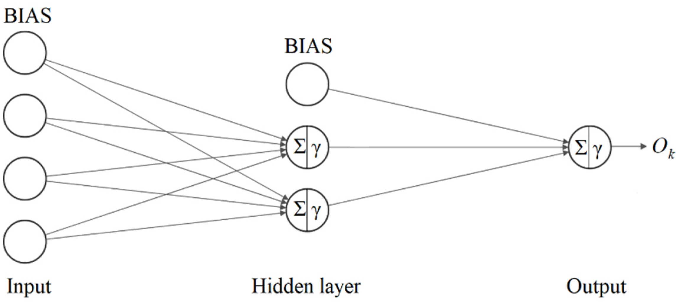
To predict the added resistance of regular head waves of a container ship, a feedforward MLP was utilized with an input, one hidden layer, an output layer, and an error backpropagation (EBP) algorithm. As already mentioned, the network has 10 inputs and one output, i.e., the coefficient of added resistance in waves. As can be seen in Figure 2, the input values multiplied by the weights were summed and passed through an activation function within each neuron of the hidden layer. The bias neuron was also included to shift the activation function, thus enabling an additional degree of freedom. The outputs of neurons $y$ within the hidden and output layer are determined as follows:

$$y=\varphi \left({\displaystyle \sum _{i=0}^n{w}_i{x}_i}\right)$$

(3)

where $\varphi$ is the activation function, $w_i$ are weights, and $x_i$ are input values. The activation function utilized to transform the neuron output is linear in the output layer, and the hyperbolic tangent sigmoid transfer function in the hidden layer is defined as follows:

$$\gamma =\frac{2}{1+e^{-2x}}-1$$

(4)

Within the training process of the neural network, the optimal weights are determined iteratively by minimizing the error function. The errors are calculated in the forward direction by the backpropagation algorithm based on the inputs and the corresponding outputs. The weights are changed in a backpropagation manner based on the minimization of the error function.

The performance of the neural network is assessed by the normalized value of the root mean square error (NRMSE), which is calculated as follows:

$$\mathrm{NRMSE}=\frac{\mathrm{RMSE}}{{\sigma }_{d_n}}=\frac{\sqrt{\frac{{\displaystyle \sum _{n=1}^N{\left(d_n-O_n\right)}^2}}{N}}}{{\sigma }_{d_n}}$$

(5)

where ${\sigma }_{d_n}$ is the standard deviation, $O_n$ is the neural network output, $d_n$ is the desired output, and $N$ is the number of samples used either for training or testing the network.

The number of neurons in the hidden layer is varied to achieve the adequate topology of the network to predict the added resistance in waves with sufficient accuracy. The hydrodynamic calculations were performed in the range of incoming wave frequencies from 0.1 to 1.5 rad/s. This resulted in 11,230 samples in total. Firstly, the network was trained based on 95% of the data in total, and 5% of the data was used for testing. Afterward, the container ships were divided into three classes based on their size. The first class contained data for ships from 104 to 155 m, the second class from 178 to 247 m, and the third class from 300 to 360 m in length. The first class contained 5086 samples, the second one contained 3456 samples, and the third one contained 2688 samples in total. Again, 95% of the data was used for training, and 5% was used for testing purposes. The network was trained based on the Levenberg–Marquardt learning algorithm with Bayesian regularization (BR). The validation data set was not established, since BR does not need the validation data. BR is superior in generalization compared to the standard EBP neural network. A nonlinear regression problem is converted into a statistical one using the probabilistic approach. It is difficult to overfit the neural network with BR, since training is conducted with a limited number of weights. The weights that are not relevant to the learning process are discarded by maximizing the posterior probability. The calculation of the Hessian matrix within BR is approximated using the Gauss–Newton method within the LM learning algorithm. The error function consists of the sum of squared errors of desired and predicted outputs $E_D$ and the sum of squared weights $E_W$ [33]:

$$F=\beta E_D+\alpha E_W$$

(6)

where $\alpha$ and $\beta$ are the regularization parameters.

The sum of squared errors is calculated as:

$$E=\frac{1}{2}{\displaystyle \sum _{n=1}^N{\left(d_n-O_n\right)}^2}$$

(7)

At the beginning of the training, the weights and the regularization parameters are initialized as 0 for $\alpha$ and 1 for $\beta$. After each iteration step of the training using the LM algorithm, a minimum of the error function $F$ is sought. The number of weights involved in the training process is determined as follows:

$$\gamma =N-2\alpha \mathrm{tr}{\left[{\nabla }^{2}F\left(w\right)\right]}^{-1}$$

(8)

where $N$ is the total number of weights, and ${\nabla }^{2}F\left(w\right)$ denotes the Hessian matrix, which is determined based on the Gauss–Newton approximation:

$${\nabla }^{2}F\left(w\right)\approx 2\beta J^{T}J+2\alpha I_N$$

(9)

New estimates of the regularization parameters are determined as:

$$\alpha =\frac{\gamma }{2E_W\left(\vartheta \right)}$$

(10)

$$\beta =\frac{n-\gamma }{2E_D\left(\vartheta \right)}$$

(11)

A neural network based on the LM learning algorithm and BR was selected for the prediction of added resistance based on its best performance amongst other investigated first- and second-order learning algorithms [27]. One of the main advantages of such a network is that most of the gathered data can be used for training purposes. The accuracy of the neural network output depends on the quality of the data used for the training. For that reason, the data has to be pre-processed and prepared for the training. This includes the removal of the possible outliers and ensuring an equivalent impact of input on output variables. Since the input variables have different ranges and dimensions, the input data were standardized, which resulted in a unit standard deviation and a zero-mean value. One of the data cleaning and pre-processing techniques that was applied is principal component analysis (PCA), which is a dimensionality reduction method that is commonly applied to eliminate the collinearity of dependent variables in a multivariate data set. By creating linearly independent principal components obtained by an eigenvalue decomposition of the data covariance matrix, PCA enables the reduction in the number of inputs while keeping as much data variance as possible. Within this study, all input variables were kept; however, they were replaced by the principal components, which improved the performance of the neural network.

5. Results

The obtained numerical results for three benchmark container ships were validated by comparison with the available experimental data [34,35]. The obtained results of the validation study for the KCS container ship are presented in Figure 3. The numerical results obtained by the BIEM and corrected at short waves were in satisfactory agreement with the experimental data. A slight shift of the numerically obtained curve of the added resistance coefficient towards lower wave frequencies could be noticed in comparison to the experimentally obtained data. However, a noticeable scatter of the experimental results could be observed as well.

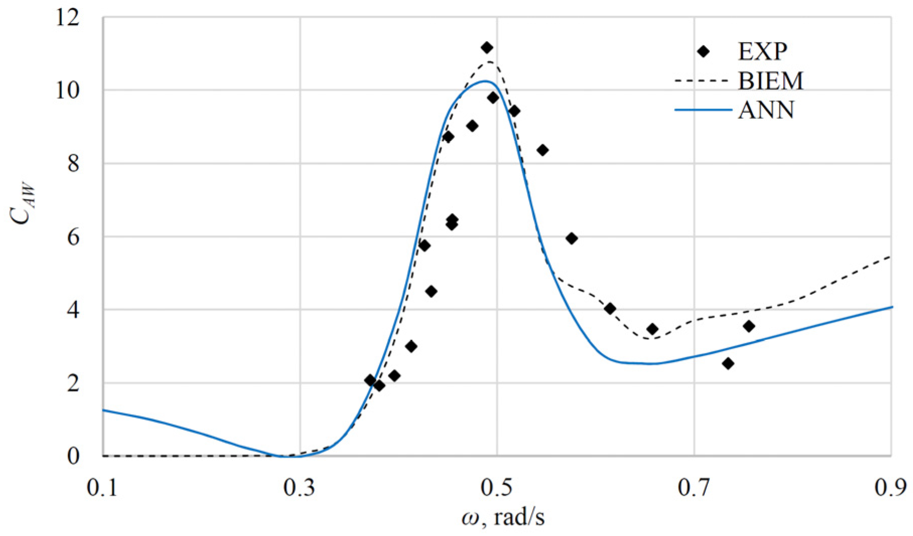
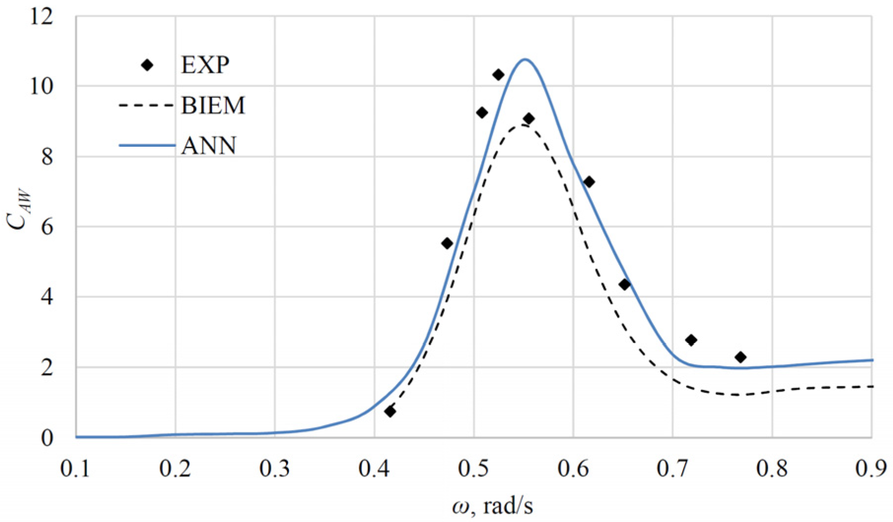
The numerically and experimentally [36] obtained results for the S175 container ship at three Froude numbers are compared and shown in Figure 4, Figure 5 and Figure 6. The numerical results at $Fr=0.20$ were in satisfactory agreement with the experimental ones, especially in the range of moderate wave frequencies around the location of the peak position. 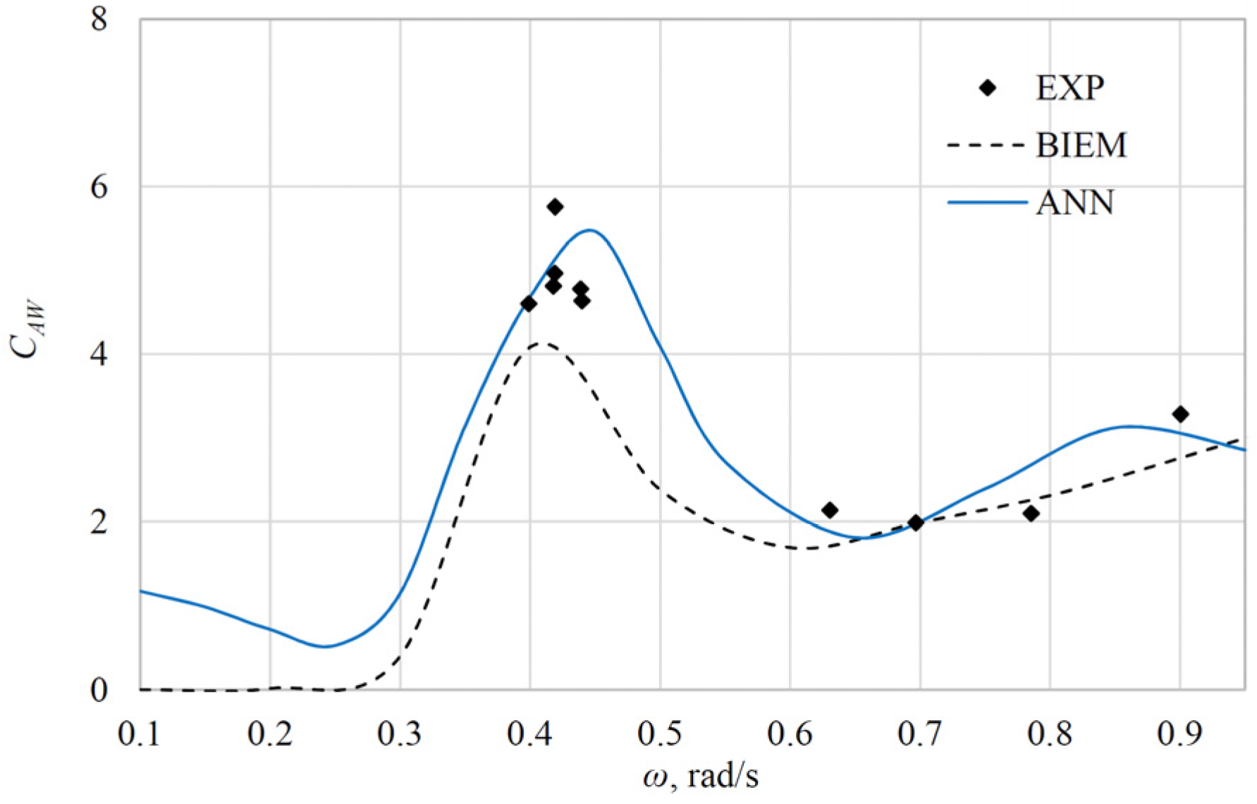In the range of higher wave frequencies, the numerical results seemed to underestimate the experimental data despite the applied correction, as shown in Figure 4. For $Fr=0.25$, the added resistance coefficient obtained numerically was underestimated for all wave frequencies, with the position of the peak value being slightly shifted towards higher wave frequencies, as shown in Figure 5. The numerical results for $Fr=0.30$ were in good agreement with the experimental data at short waves, where the experimental data were more consistent, as shown in Figure 6. The experimental data showed a significant scatter in the range of moderate wave frequencies, which makes proper comparison between the results troublesome. For the DTC, which represents a modern post-Panamax container ship [10], it can be seen that BIEM notably underestimated the added resistance coefficients for the wave frequencies around the peak position, as shown in Figure 7.

Once all numerical calculations were performed and the outliers were removed, the numerically obtained data were standardized, and PCA was carried out. Based on a detailed inspection of the gathered data, some of the results were discarded as the potential cause of the noise. Namely, for some ships, the appearance of irregular frequencies was noticed at lower frequencies than expected, which means that those results had to be removed from the training and testing data set.

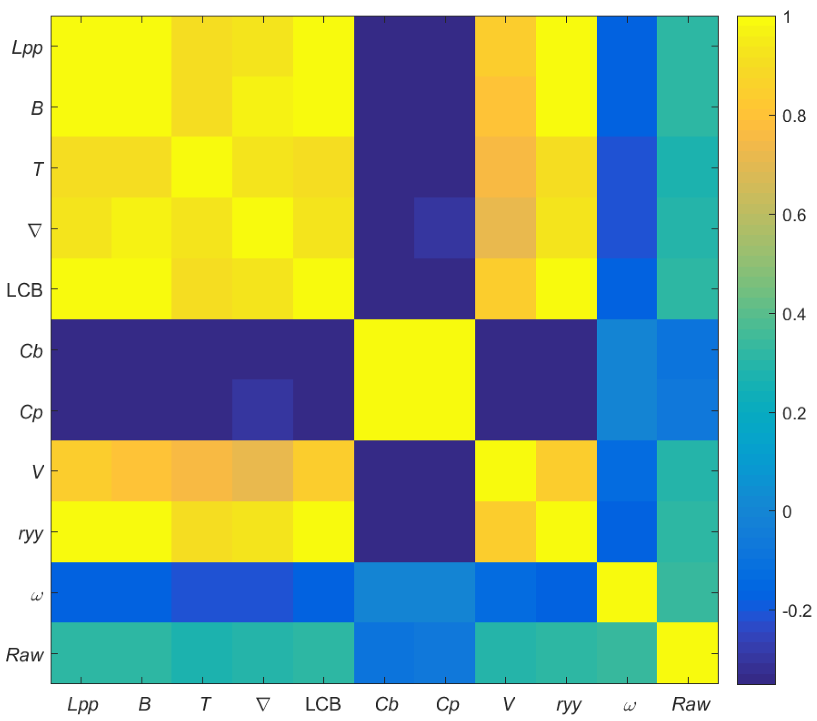
To represent the linear correlation between the input variables, the Pearson correlation coefficient was used [37]. The correlation between the input variables and the added resistance coefficient as the output is given as a heat map in Figure 8. A moderate correlation between all input variables, except for the block and prismatic coefficients, as well as the added resistance in waves, can be observed. The hull form coefficients correlated poorly with the added resistance in waves. On the other hand, a strong correlation between the block and prismatic coefficient can be observed, as well as a moderate correlation between those coefficients and other hull characteristics and speed.

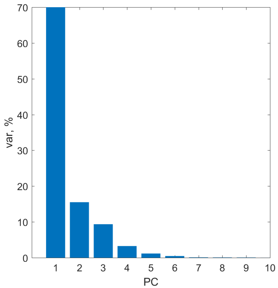
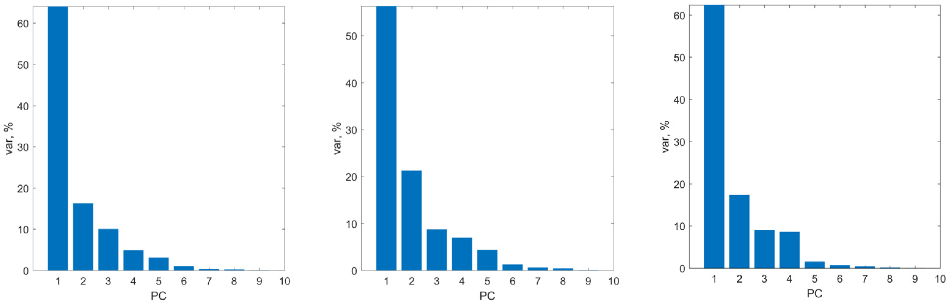
The principal components and the percentage of variance in each of them can be seen in Figure 9. It should be noted that the total variance contained in the first five principal components was equal to 99.3%, which would potentially enable the reduction in the number of input variables. It is worth mentioning that the learning process based on the linearly independent variables was significantly accelerated. In Figure 10, the variance that can be explained by principal components for the three container ship classes is shown. The obtained results for the first and third class were very similar, while the second principal component for the second class contained somewhat more information in comparison to the other two classes. The output data was normalized before training, thus resulting in a range of added resistance coefficients from 0 to 1.

During the supervised training, the weights were iteratively updated based on the LM algorithm by minimizing an error function, and the NRMSE of the training and testing data set was monitored. The data used for testing purposes consisted of 5% of the numerically obtained data and the experimental data for the benchmark container ships. Based on the performance of neural networks with different topologies, i.e., the number of neurons in the hidden layer, the neural network with 50 neurons in the hidden layer was the most successful one. The NRMSE of the training and testing data, as well as the number of iterations, are given in

Table 3. The main particulars of KCS.

Number of Neurons	Number of Iterations	NRMSE (Training)	NRMSE (Testing)
20	511	0.1331	0.1290
30	1187	0.0956	0.0923
40	1367	0.0745	0.0743
45	1487	0.0724	0.0707
50	2050	0.0662	0.0628
55	2537	0.0624	0.0633
60	2987	0.0575	0.0605

. It can be seen that, as the number of neurons within the hidden layer increased, the error decreased. In other words, the neural network adapted better to the data used within the training while avoiding overfitting. Generally speaking, the NRMSE of the testing data was lower for topologies with up to 50 neurons in the hidden layer, unlike for the neural networks with 55 and 60 neurons. It should be noted that, for these neural networks, the NRMSE of the data used for testing was lower in comparison to the NRMSE of the training data, which means that the neural network has a good generalization ability. The selected neural network topology was the one with 50 neurons in the hidden layer, which adapted well to the testing data while keeping its parsimony characteristics. That does not mean that neural networks with 55 and 60 neurons in the hidden layer have poor generalization ability. It can be noticed that the NRMSE of the testing data for a neural network with 60 neurons in the hidden layer was the lowest among all analyzed topologies.

The number of weights effectively involved in the training was 588 of 601 parameters in total. For comparison purposes, the NRMSE of the neural network with 50 neurons in the hidden layer with the LM learning algorithm without BR was 0.0895 for the training and 0.0948 for the testing data. The NRMSE for the training and testing data was 0.2419 and 0.2421, respectively when the Scaled Conjugate Gradient algorithm was used, while the learning algorithm based on Steepest Gradient Descend showed a significantly larger error and was discarded from the analysis.

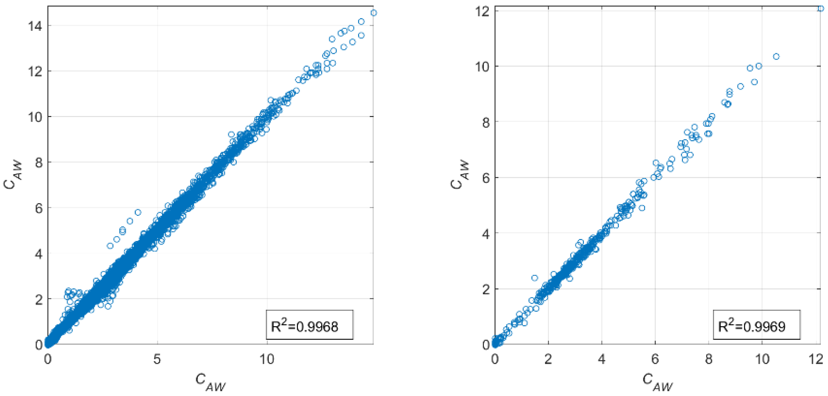
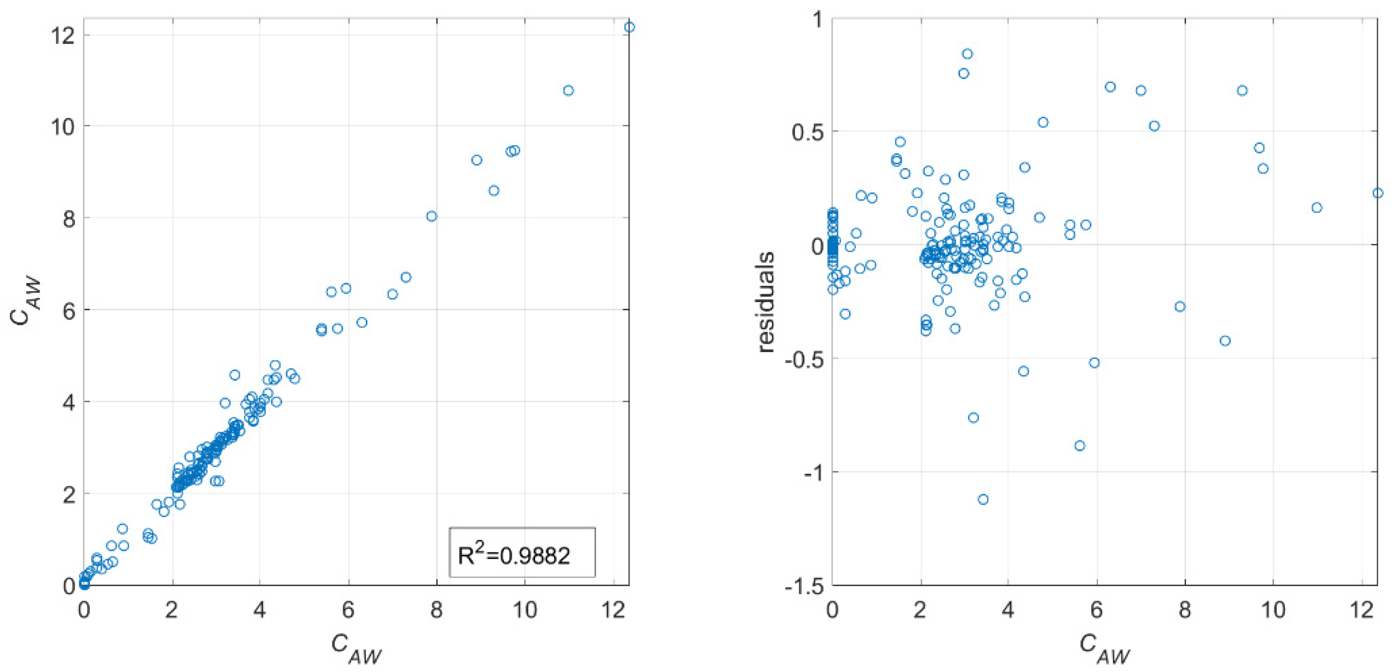
The regression plots for the training and testing data for a neural network with 50 neurons in the hidden layer are shown in Figure 11. In the case of the data used for training, some outliers can be noticed for lower values of added resistance coefficient, despite the careful pre-processing of the data. A high coefficient of determination was obtained for both the training and testing data. Based on the testing data, it can be seen that the added resistance coefficients were well-predicted without significant deviations.

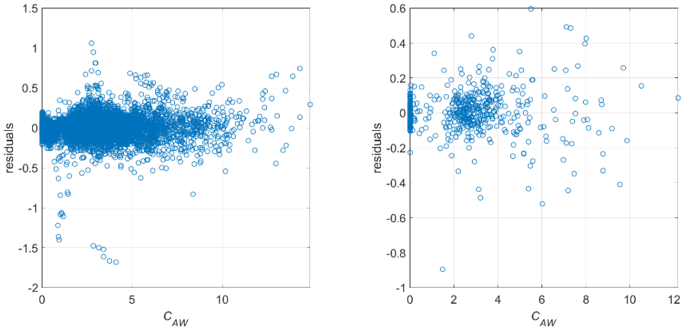
The residuals calculated as the difference between the desired output and the one obtained by the neural network for the training and testing data are presented in Figure 12. They should be inspected to validate the performance of a regression model and assess whether the error is stochastic and without any visible pattern. As can be seen from Figure 12, the residuals were uniformly distributed. However, similar to the regression plot for the training data, the outliers within the lower values of the added resistance coefficient can be noticed. Some of the possible reasons for that lie in the incorrect results of the hydrodynamic calculations or an unintentional mistake made in the data pre-processing. The residuals of the testing data were uniformly distributed as well, and the mean relative deviation between the obtained results was equal to −1.42%. Despite the outliers, the established neural network had good generalization ability. The performance of the neural network with a LM learning algorithm and BR with 50 neurons in the hidden layer for the prediction of the added resistance coefficient of the benchmark container ships is given in Figure 3, Figure 4, Figure 5, Figure 6 and Figure 7.

The neural network predicts added resistance coefficient for the KCS with sufficient accuracy, especially in the range of moderate wave frequencies. The peak value was somewhat lower in comparison to the numerically obtained results, while the values at short waves were underestimated, as shown in Figure 3. It can be observed that, instead of approaching zero, the curve of the added resistance coefficient obtained by the neural network tended to rise. For the S175, significantly better agreement between the experimental results and the ones obtained using the neural network was obtained for an $Fr=0.20$, as shown in Figure 4. The added resistance coefficient was much better predicted, even though the peak position was again slightly shifted towards the lower frequencies. Similar results can be observed for an $Fr=0.25$, as shown in Figure 5, where the peak position was shifted towards the higher wave frequencies, even though the peak value predicted by the neural network was closer to the experimentally obtained one in comparison to the numerical result. Generally speaking, the added resistance coefficient predicted by the neural network was somewhat larger in the entire frequency range compared to the numerically obtained one and in that way shows a closer agreement to the experimental results. For an $Fr=0.30$, the peak value of the added resistance coefficient was larger when predicted with a neural network in comparison to the numerically obtained result, and its position was shifted towards the lower frequencies, as shown in Figure 6. Similar to the KCS, the coefficient of added resistance in the waves slightly increased at low wave frequencies. The possible reason for this anomaly could lie in the noise of the data gathered for training, which led the neural network to predict an increase in the added resistance at such low frequencies. The added resistance coefficient for the DTC predicted by the neural network is shown in Figure 7. Again, the peak value and its position were wrongly predicted, and the trend of the curve at higher wave frequencies did not correspond to the one obtained numerically and experimentally. Again, instead of the decreasing trend of the added resistance coefficient at low frequencies, the trend was the opposite. It can be seen that the network failed to predict the added resistance for the DTC, which was a large post Panamax ship with a relatively low sailing speed of 16 knots. Within the data gathered for the training, the number of samples representing large ships with higher sailing speeds was the lowest.

To improve the obtained results and establish a model that could be readily used, the data were divided into three classes. Training the neural network based on the lower number of samples that contained similar information within the classes enabled a reduction in the number of neurons within the hidden layer. In that way, a model that could be easily implemented and used was proposed. The model contains three neural networks, each for a particular class of container ships based on their length. For each class, four network topologies were analyzed, i.e., five, six, seven, and eight neurons in the hidden layer. In that way, the expressions used to estimate the added resistance coefficient were not too complex, while there was still a sufficient number of neurons in the hidden layer to describe the given phenomenon. All three neural networks were trained based on the LM learning algorithm with BR. The obtained NRMSE, along with the number of iterations for different network topologies, are given in

Table 4. The results obtained for different neural network topologies for three data classes.

Class	Number of Neurons	Number of Iterations	NRMSE (Training)	NRMSE (Testing)
1	5	555	0.1273	0.1534
	6	461	0.1151	0.1185
	7	535	0.1138	0.136
	8	459	0.1124	0.1333
2	5	176	0.123	0.1379
	6	83	0.1114	0.115
	7	166	0.1097	0.1075
	8	140	0.1082	0.111
3	5	40	0.105	0.0987
	6	83	0.0838	0.0783
	7	174	0.0761	0.0701
	8	49	0.0912	0.0903

. For class 1, the neural network with six neurons in the hidden layer was selected. It had the lowest NRMSE for the testing data. It can be seen that, despite the decrease in the NRMSE for the training data, the network adapted better to the data used for training, while the error of the testing data increased. The neural network with seven neurons in the hidden layer was chosen to predict the added resistance coefficient for class 2, with the NRMSE for the testing data equal to 0.1075. The network with the same topology was established for class 3 as well, which yielded the lowest NRMSE for both the training and testing data set. From Table 3, it can be seen that, by increasing the number of neurons within the hidden layer by one, the NRMSE for the training and testing data notably increased as well. In comparison to the results obtained using the neural network trained by the unclassified data, it can be noticed that the errors obtained for both the training and testing data were significantly larger. In other words, the network did not adapt to the data that well; however, it kept its generalization ability while being much less complex and easier to implement.

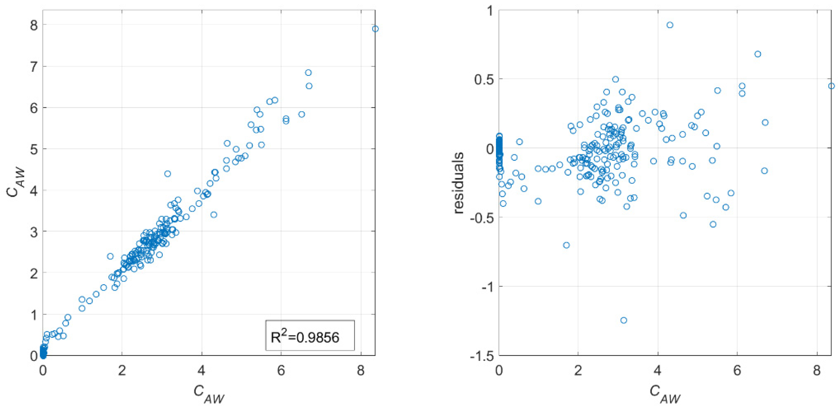
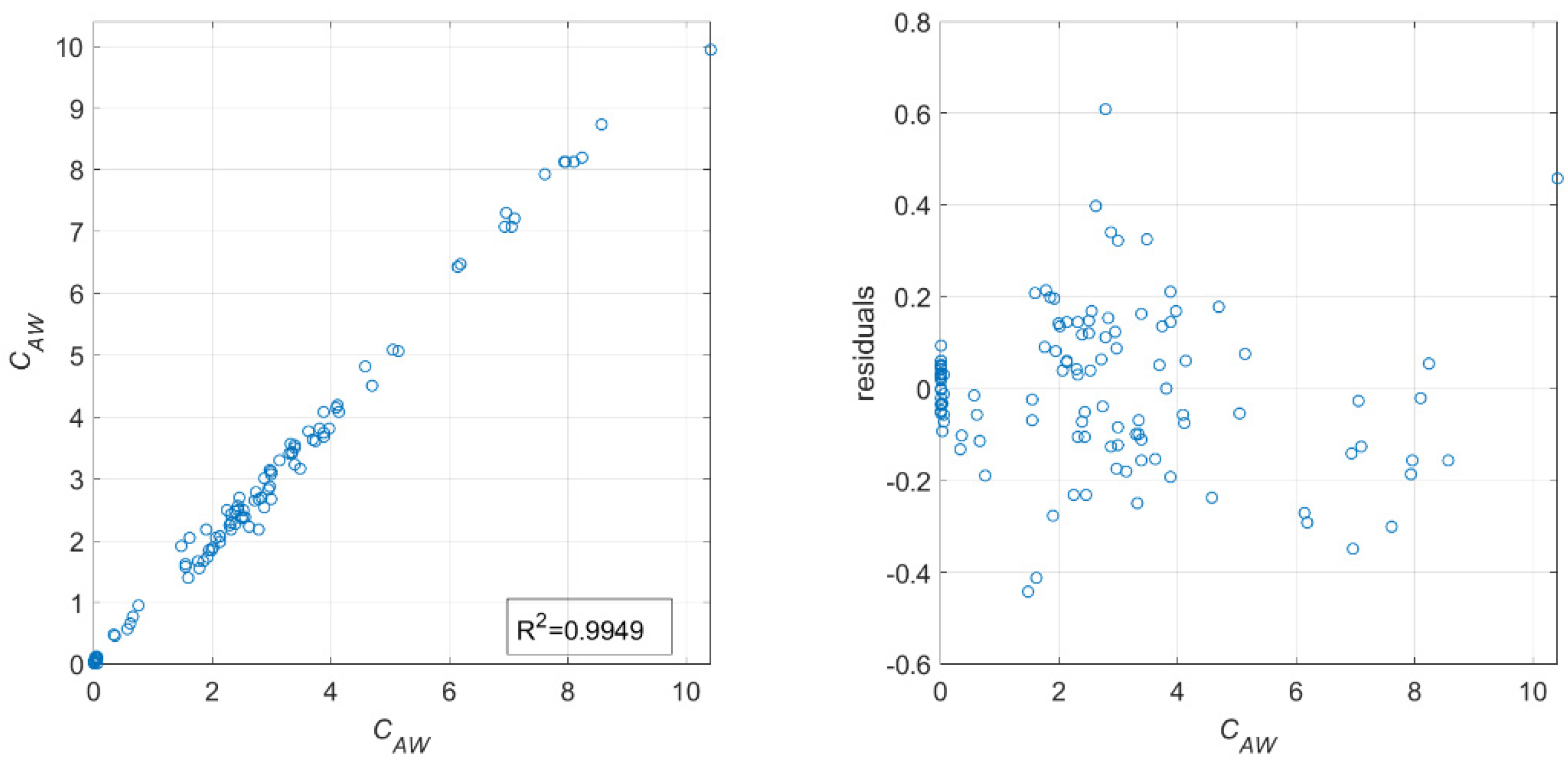
The regression plots and residuals for the testing data for all three neural networks are given in Figure 13, Figure 14 and Figure 15. In the case of class 1, the coefficient of determination was equal to 0.9856, and the residuals were randomly distributed, as shown in Figure 13. In comparison to the residuals obtained by the neural network trained by unclassified data, it can be seen that the range of residuals for class 1 was larger. Some outliers can be seen in both the regression and residual plots. A slightly larger coefficient of determination was obtained for class 2, as shown in Figure 14. The residuals were in the same range as the ones for class 1. It should be noted that the values of added resistance coefficient for class 2 were the largest in comparison to the other two classes. As already shown in the comparison between the numerically and experimentally obtained added resistance coefficients for the DTC container ship, which by length belongs to class 3, the BIEM underestimated the added resistance. The same can be observed by comparing the regression plots for classes 2 and 3, which are shown in Figure 14 and Figure 15. However, it is worth noting that the residuals obtained for class 3 were lower in comparison to the other two classes, and the coefficient of determination was the largest.

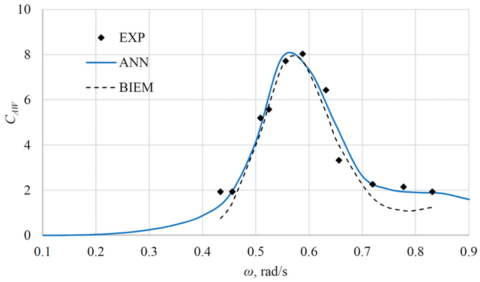
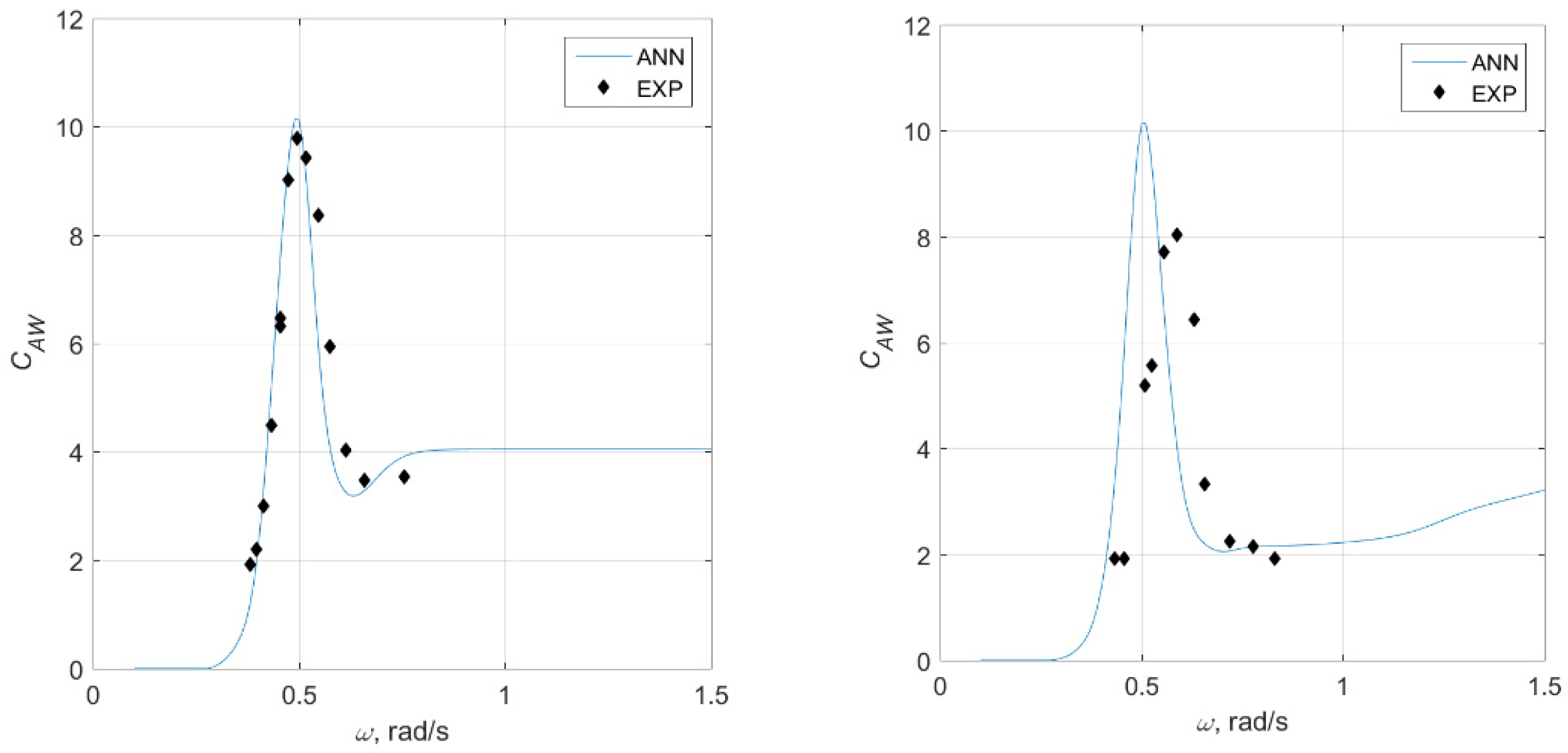
Since the KCS and S175 container ships belong to class 2 by their length, the added resistance coefficient was predicted by the second neural network with seven neurons in the hidden layer. The obtained results are presented in Figure 16. In the case of the KCS, a very good agreement between the network output and the experimental data can be seen. However, the network output for very the high wave frequencies was almost constant. 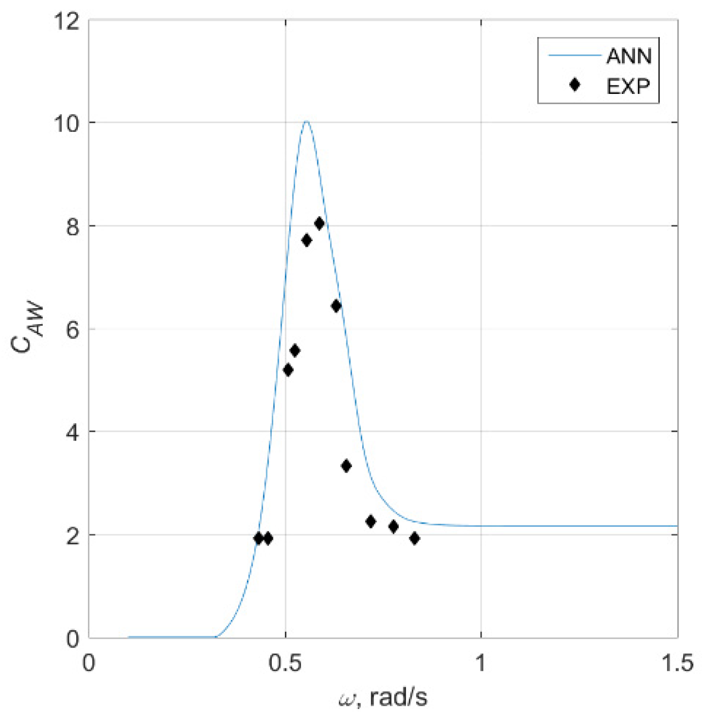In the case of the S175 container ship for an $Fr=0.20$ it can be noticed that the network significantly overestimated the added resistance, while the peak was slightly shifted to the lower wave frequencies. Since this Froude number was at the bottom boundary for ship speed for class 2, the added resistance coefficient for the S175 was estimated by the first neural network as well, as shown in Figure 17. It is interesting to observe how the peak values obtained by the first and second neural networks were almost the same. On the other hand, the peak position predicted by the first neural network was more accurate.

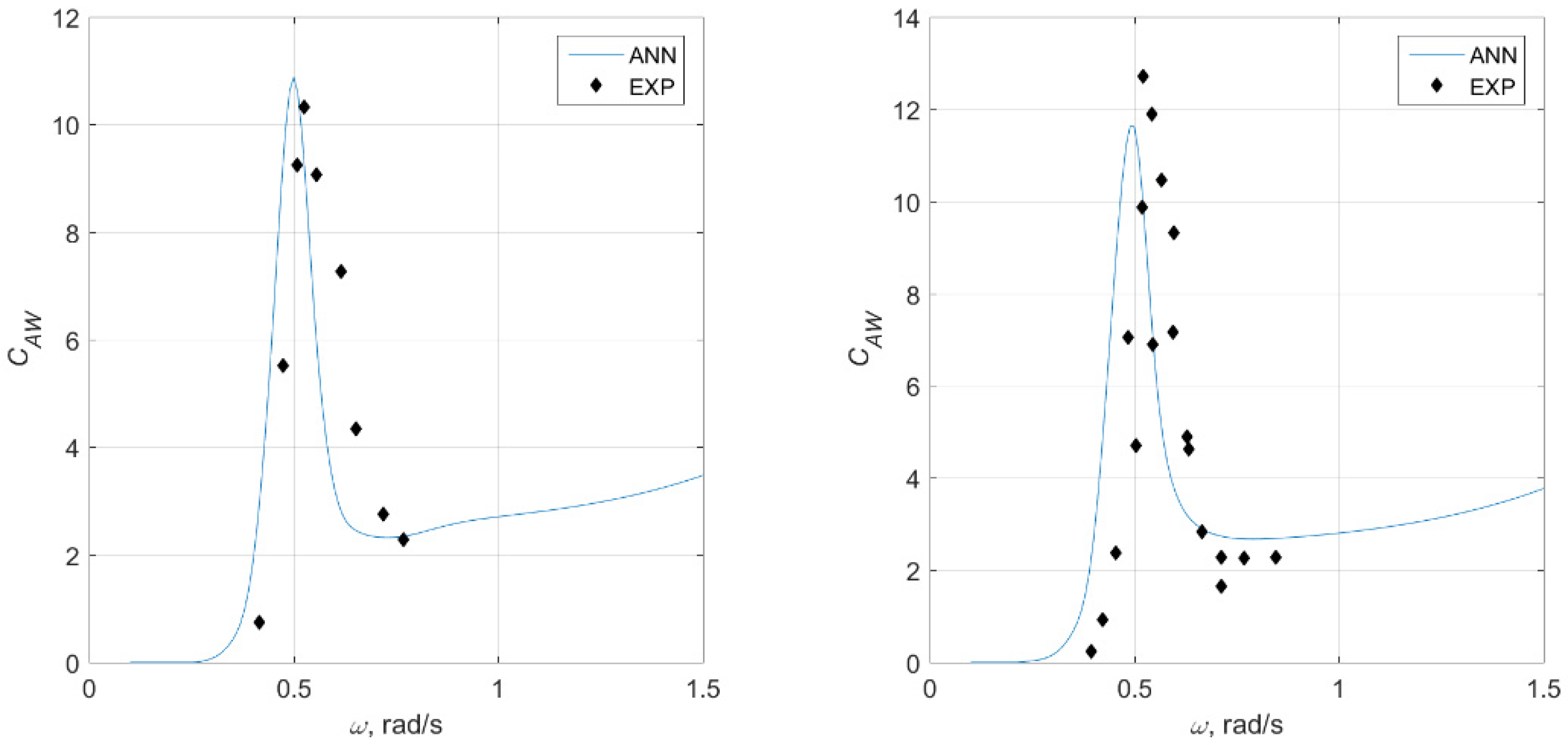
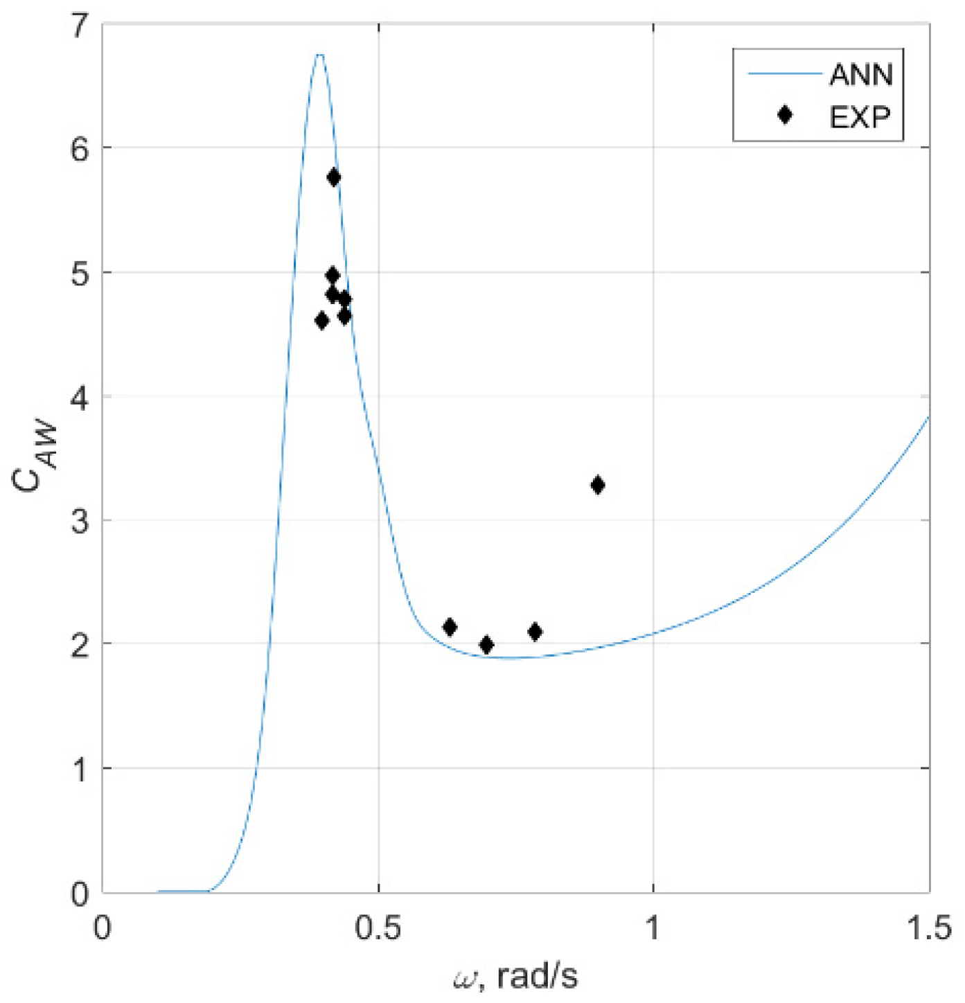
The values for the other two investigated Froude numbers for the S175 container ship were in much better agreement with the experimental data, as shown in Figure 18. Again, the curve of the added resistance coefficient for both Froude numbers, i.e., an $Fr=0.25$ and an $Fr=0.30$, was slightly shifted towards the lower wave frequencies. The added resistance coefficients predicted by the third neural network for the DTC container ship were overestimated around the peak area, as shown in Figure 19. In addition, the peak position of the added resistance curve was not predicted accurately by the neural network, as obtained in [2].

The expressions for the prediction of the added resistance coefficient for all three neural networks are given in the Appendix A, Appendix B and Appendix C, and of this paper, and the ranges of the container ships’ characteristics for all three container ship classes are given in

Table 5. Ranges of the container ships’ characteristics for all classes.

Main Particular	Range for Class 1	Range for Class 2	Range for Class 3
$L_{PP}$, m	$104.8÷155.4$	$178÷247$	$300÷360$
$B$, m	$18÷25$	$25.85÷32.26$	$37÷49$
$T$, m	$4.25÷9.2$	$8÷12$	$11÷15$
$\nabla$, m3	$5648.7÷\mathrm{22,672}$	$\mathrm{23,326}÷\mathrm{67,343}$	$\mathrm{67,244}÷\mathrm{174,090}$
$C_B$	$0.562÷0.780$	$0.51÷0.75$	$0.53÷0.65$
$C_P$	$0.569÷0.811$	$0.53÷0.768$	$0.569÷0.672$
LCB, m	$49÷77.7$	$87.5÷121$	$140.9÷180.7$
$k_{yy}$, m	$25.15÷40.4$	$42.72÷64.22$	$72÷93.6$
$V$, kn	$12.1÷19$	$17.3÷24$	$19.1÷26$

.

6. Conclusions

Within this paper, an artificial neural network was used for the prediction of the added resistance in regular head waves. The data used for training and testing the artificial neural network were gathered by performing the calculations based on the Boundary Integral Element Method for various container ships at different speeds. The numerically obtained data were validated against the experimental data available in the literature. Prior to training the neural network, the data was pre-processed, and the outliers were removed. Because of the appearance of the irregular frequencies, some of the obtained numerical results were discarded from the training and testing data set. The neural network was trained based on the Levenberg–Marquardt learning algorithm with Bayesian regularization. Firstly, 95% of all numerical results were used for training the network, and the topology of 50 neurons in the hidden layer proved to be the most successful one. To simplify the neural network model, the numerical data was divided into three classes based on the container ship length. In that way, for each container ship class, a simple and easy-to-implement model was established. The performance of all three neural networks was demonstrated for three benchmark container ships. The proposed model can be readily used to predict the added resistance coefficient for container ships in regular head waves of frequencies in the range from 0.1 to 1.5 rad/s, and, in that way, the limited availability of the experimental results, when it comes to the range of incoming frequencies, can be overcome. The limitations of the proposed model are the ranges of the container ship particulars and the Froude number, as well as the wave direction, since only the head waves were considered. A simple and efficient model for the rapid determination of added resistance was proposed, which can be used within preliminary ship design. Unlike the hydrodynamic calculations, it does not require a 3D model of the ship hull, and it only requires a model of the main particulars.