Author Contributions
Conceptualization, C.G.G., N.D. and I.M.; methodology, C.G.G., N.D. and I.M.; software, C.G.G.; validation, C.G.G., N.D. and I.M.; formal analysis, C.G.G., N.D. and I.M.; investigation, C.G.G., N.D. and I.M.; resources, N.D.; writing—original draft preparation, C.G.G., N.D. and I.M.; writing—review and editing, C.G.G., N.D. and I.M.; visualization, C.G.G.; supervision, N.D.; project administration, C.G.G., N.D. and I.M. All authors have read and agreed to the published version of the manuscript.
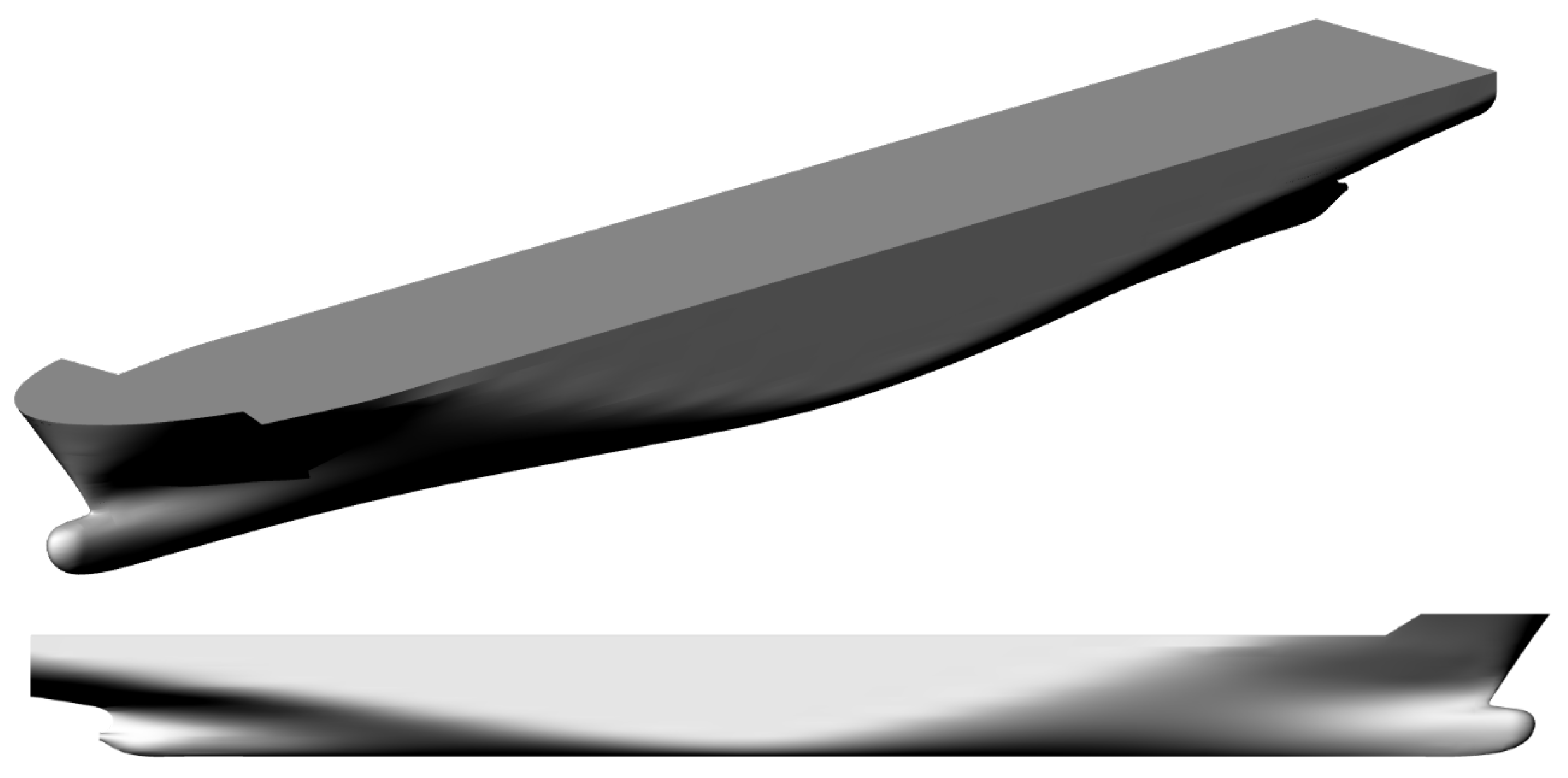
Figure 1.
Geometry of the post-Panamax 6750-TEU container ship.
Figure 1.
Geometry of the post-Panamax 6750-TEU container ship.
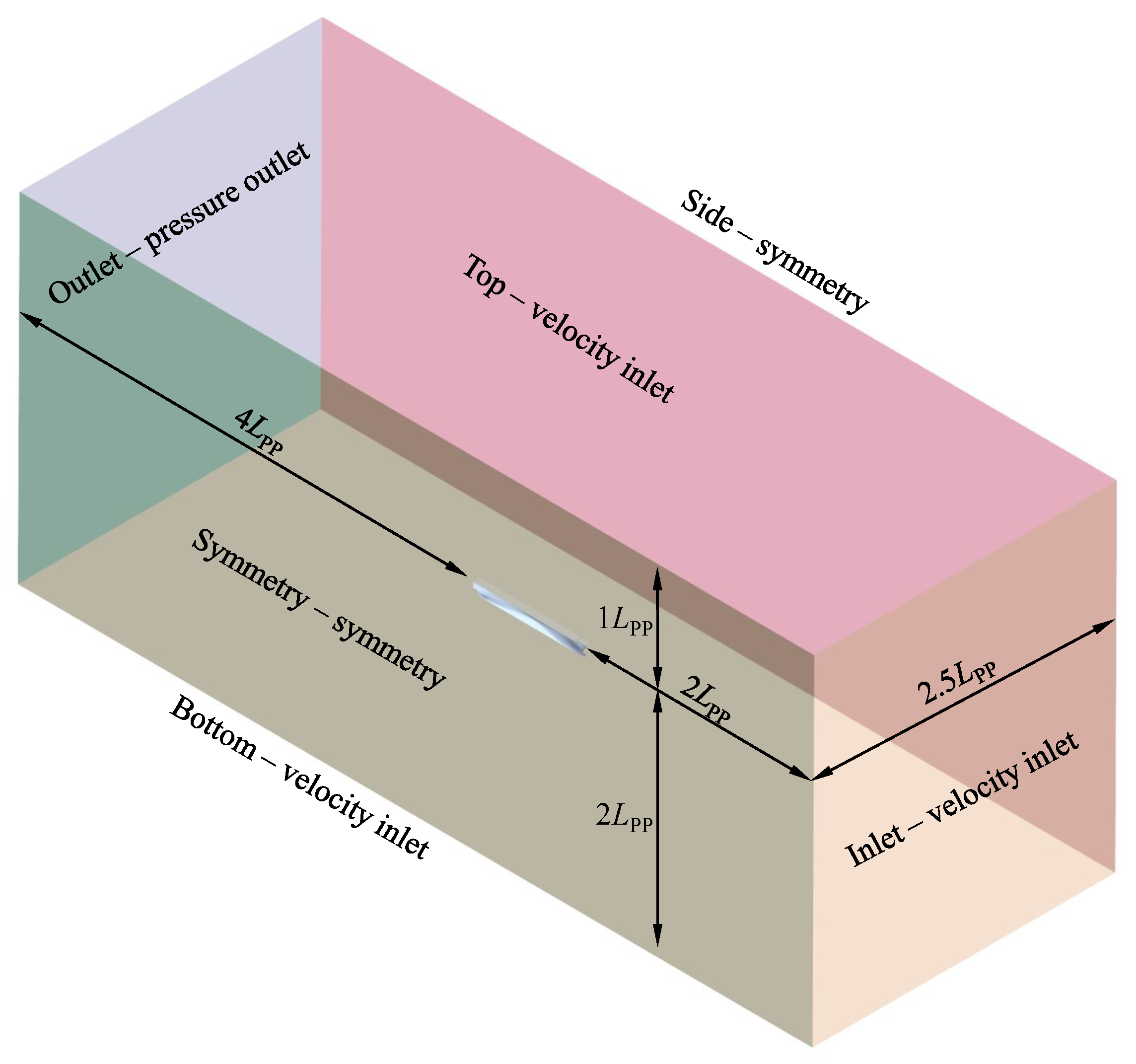
Figure 2.
Dimensions and boundaries of the computational domain for the free surface simulations.
Figure 2.
Dimensions and boundaries of the computational domain for the free surface simulations.
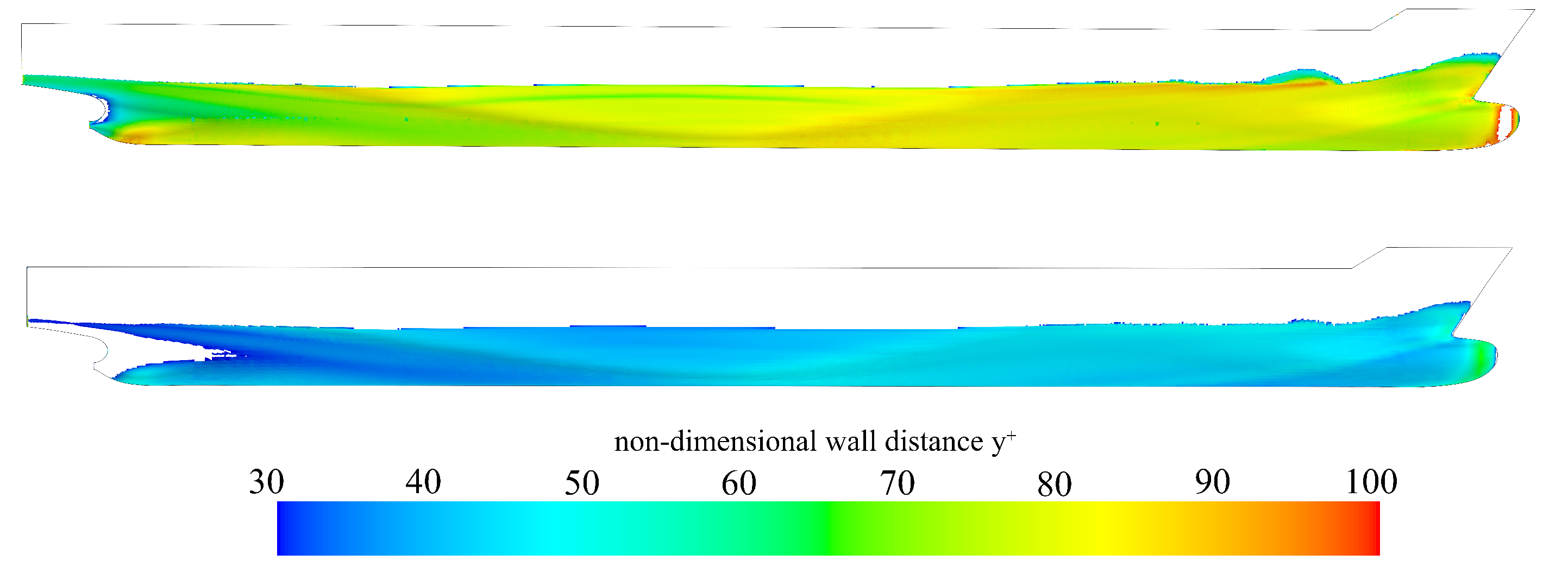
Figure 3.
Distribution of the non-dimensional wall distance on the full scale (top) and model scale (bottom) hull surface.
Figure 3.
Distribution of the non-dimensional wall distance on the full scale (top) and model scale (bottom) hull surface.
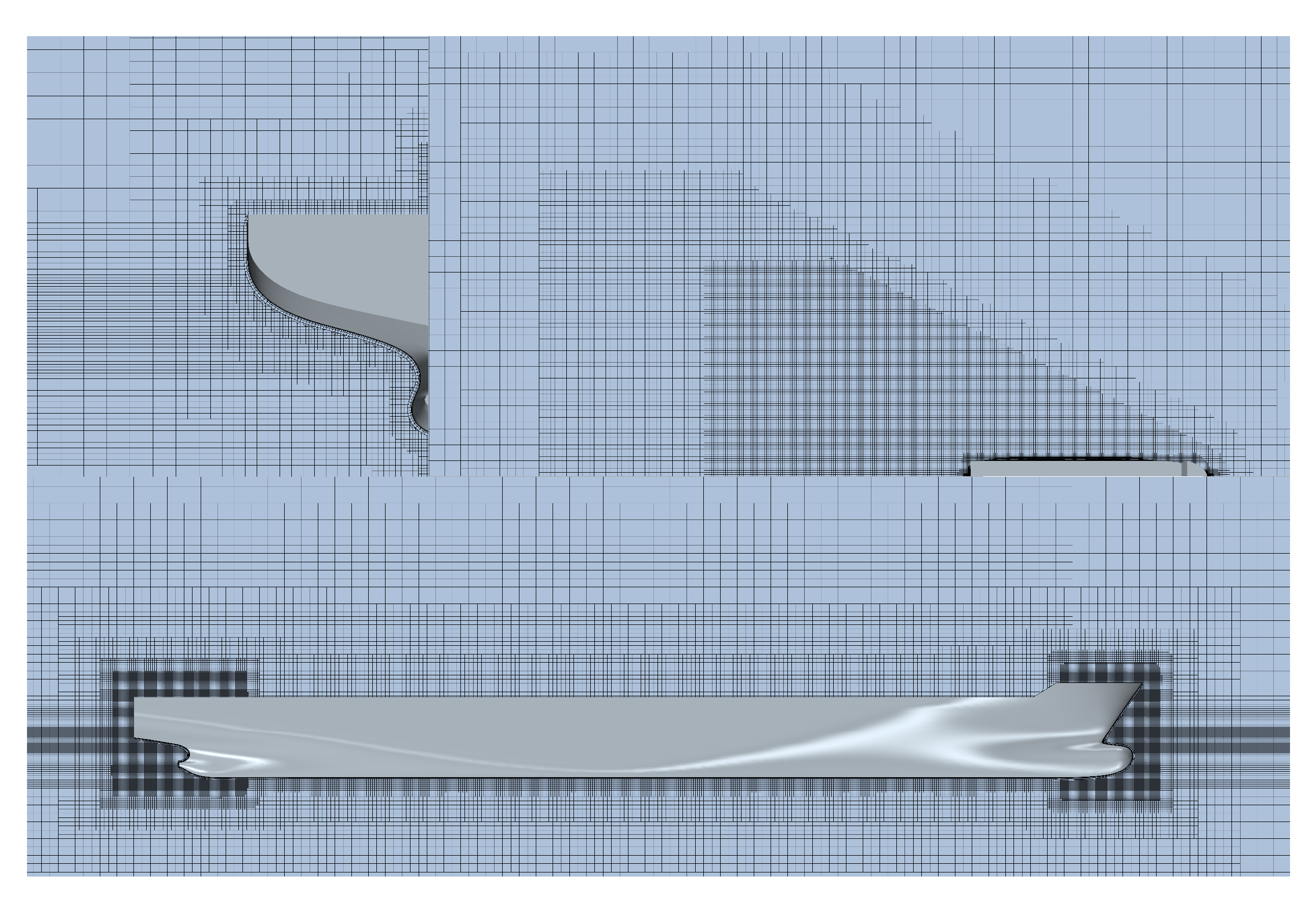
Figure 4.
Fine grid with refinements.
Figure 4.
Fine grid with refinements.
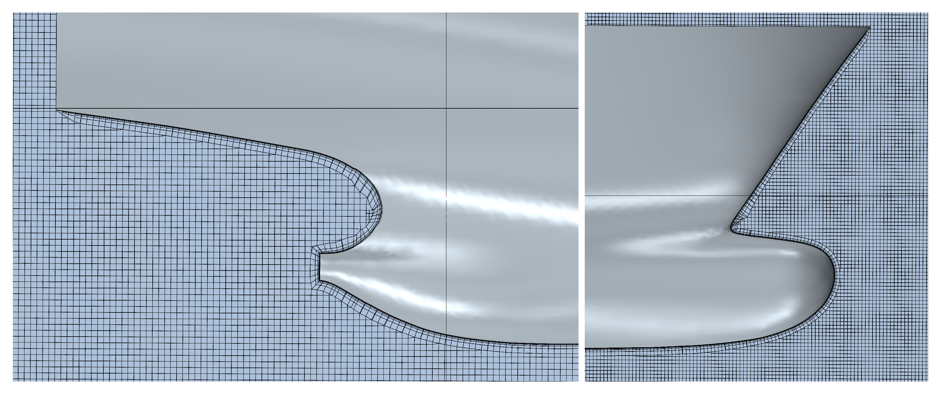
Figure 5.
Detailed view of the prism layers at the stern (left) and bow (right).
Figure 5.
Detailed view of the prism layers at the stern (left) and bow (right).
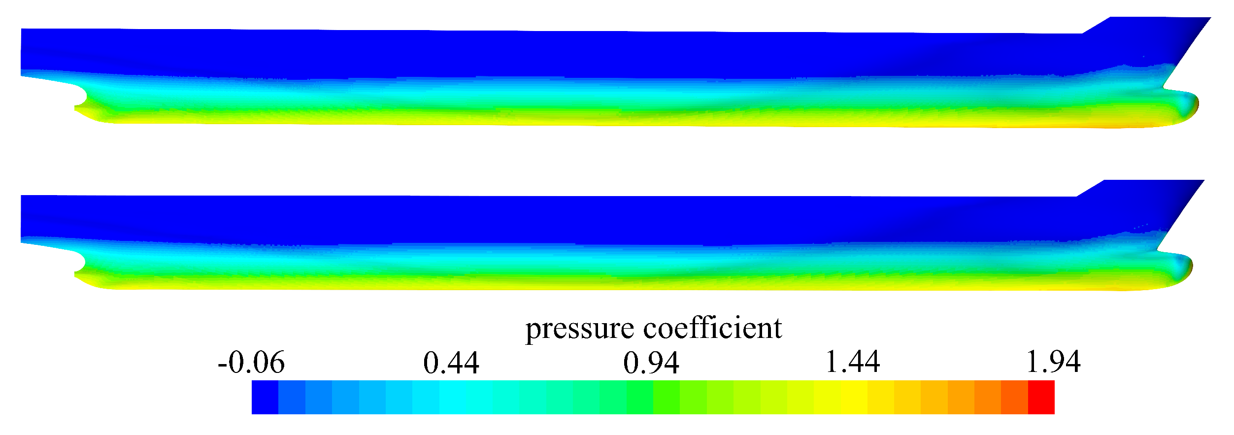
Figure 6.
Distribution of the pressure coefficient on the hull surface at full scale (top) and model scale (bottom).
Figure 6.
Distribution of the pressure coefficient on the hull surface at full scale (top) and model scale (bottom).
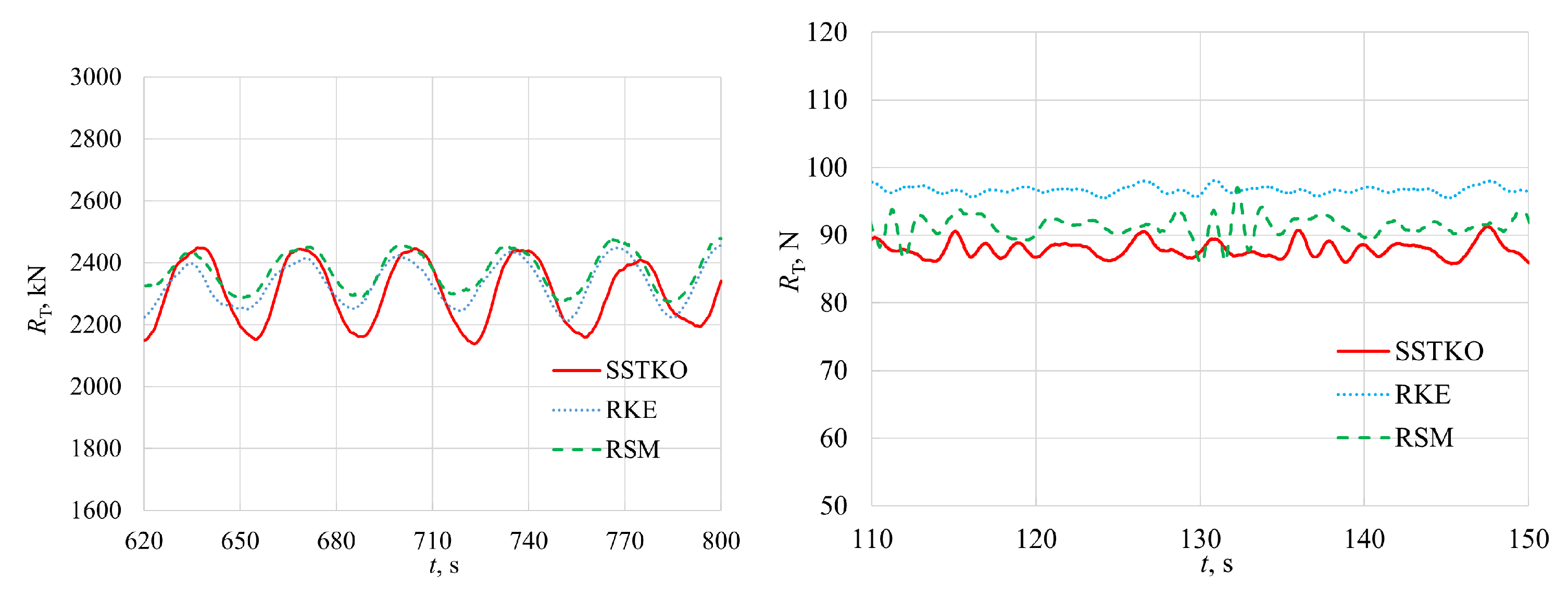
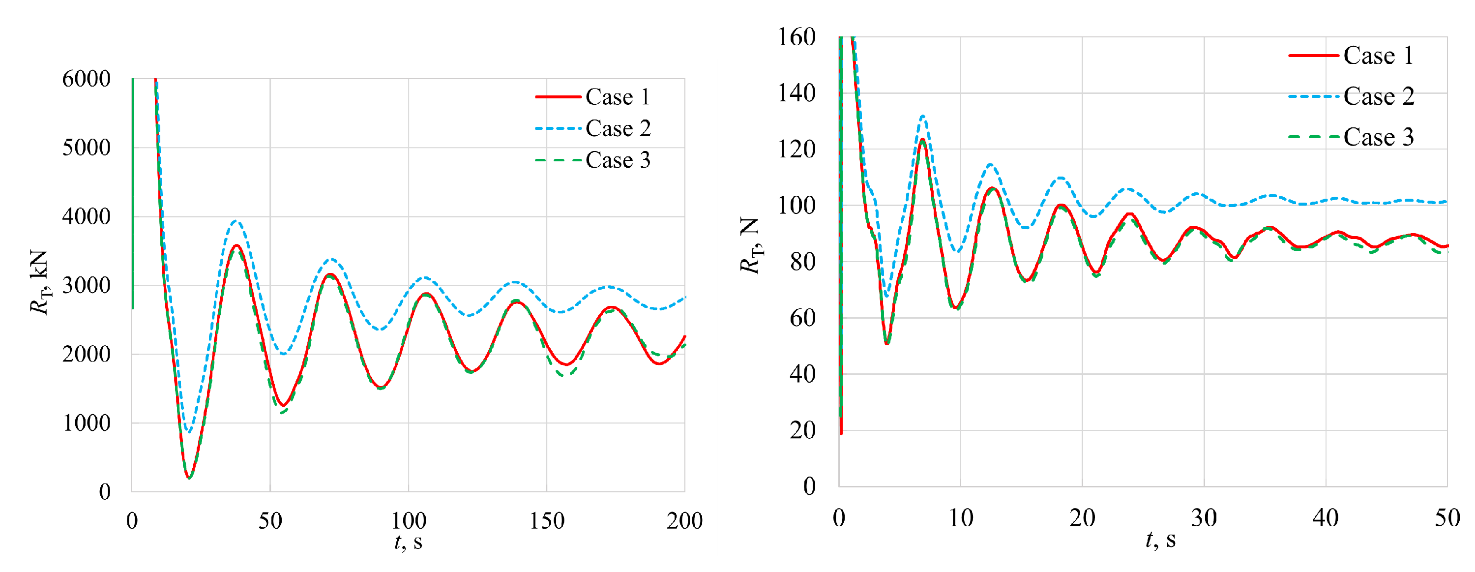
Figure 7.
Comparison of total resistance obtained using three turbulence models at full scale (left) and model scale (right).
Figure 7.
Comparison of total resistance obtained using three turbulence models at full scale (left) and model scale (right).
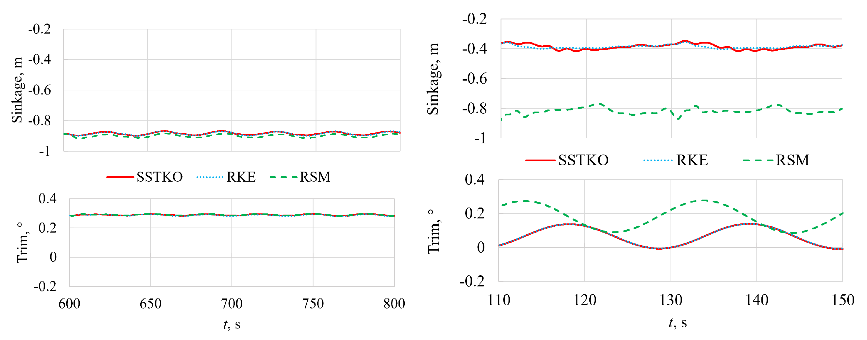
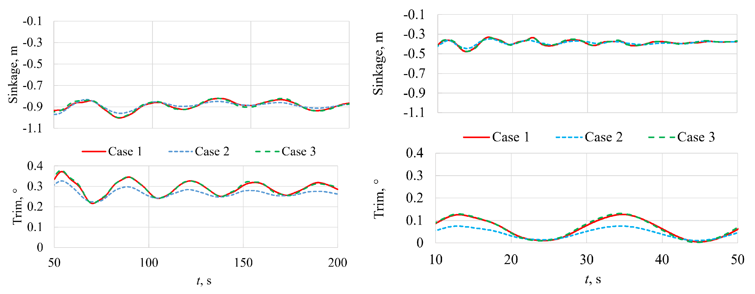
Figure 8.
Sinkage and trim values as a function of physical time for three turbulence models at full scale (left) and model scale (right).
Figure 8.
Sinkage and trim values as a function of physical time for three turbulence models at full scale (left) and model scale (right).
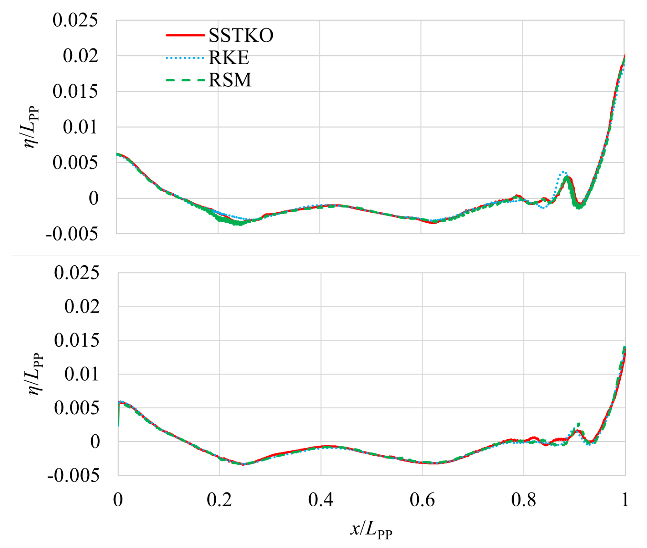
Figure 9.
Wave elevations along the hull at full scale (top) and model scale (bottom) for different turbulence models.
Figure 9.
Wave elevations along the hull at full scale (top) and model scale (bottom) for different turbulence models.
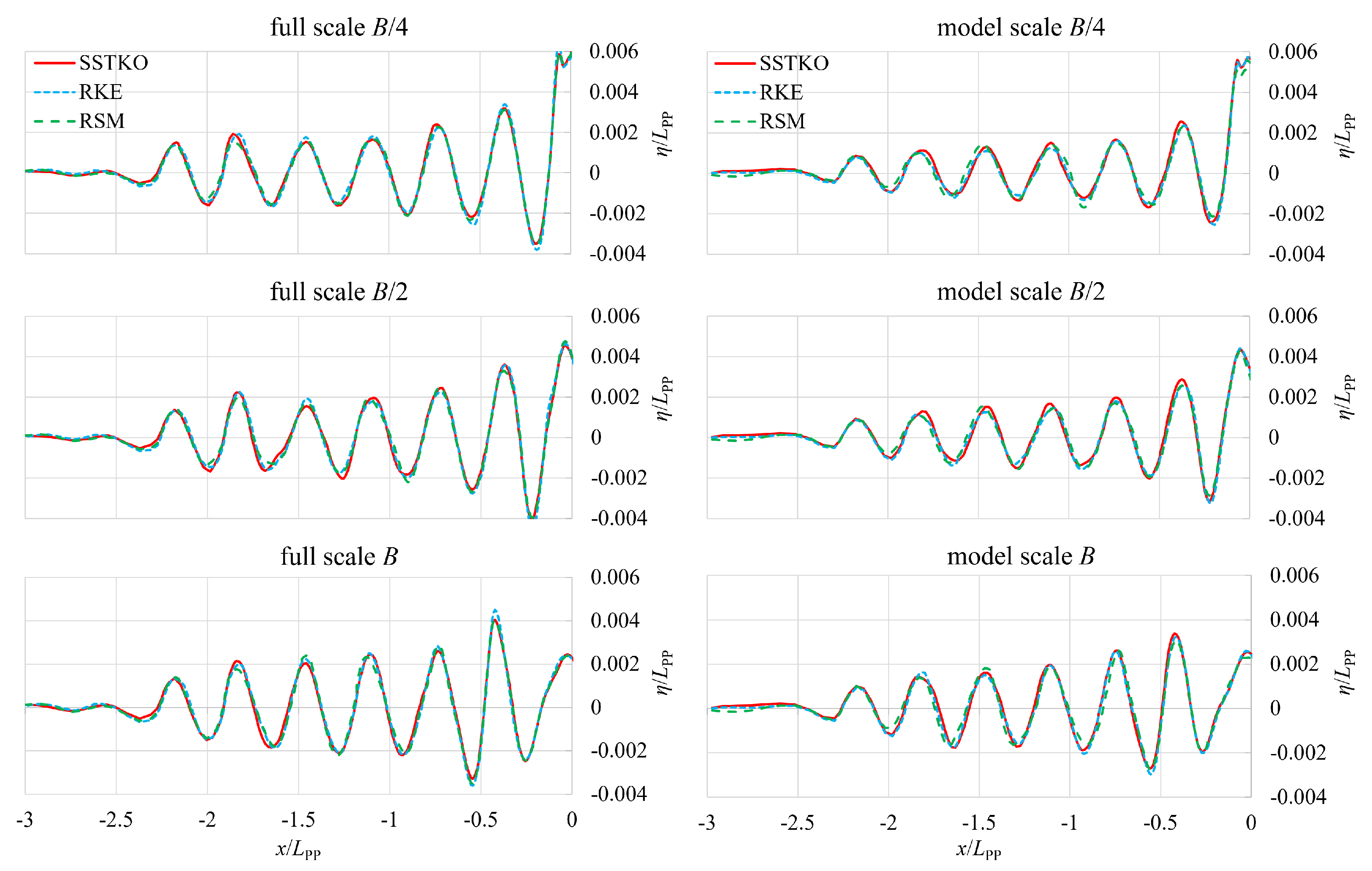
Figure 10.
Wave elevations behind the stern at longitudinal cuts , and B from the centreline of the ship obtained with numerical simulations at full scale (left) and model scale (right).
Figure 10.
Wave elevations behind the stern at longitudinal cuts , and B from the centreline of the ship obtained with numerical simulations at full scale (left) and model scale (right).
Figure 11.
Comparison of three discretization schemes for convection terms at full scale (left) and model scale (right).
Figure 11.
Comparison of three discretization schemes for convection terms at full scale (left) and model scale (right).
Figure 12.
Sinkage and trim values as a function of physical time for different discretization schemes for convection terms at full scale (left) and model scale (right).
Figure 12.
Sinkage and trim values as a function of physical time for different discretization schemes for convection terms at full scale (left) and model scale (right).
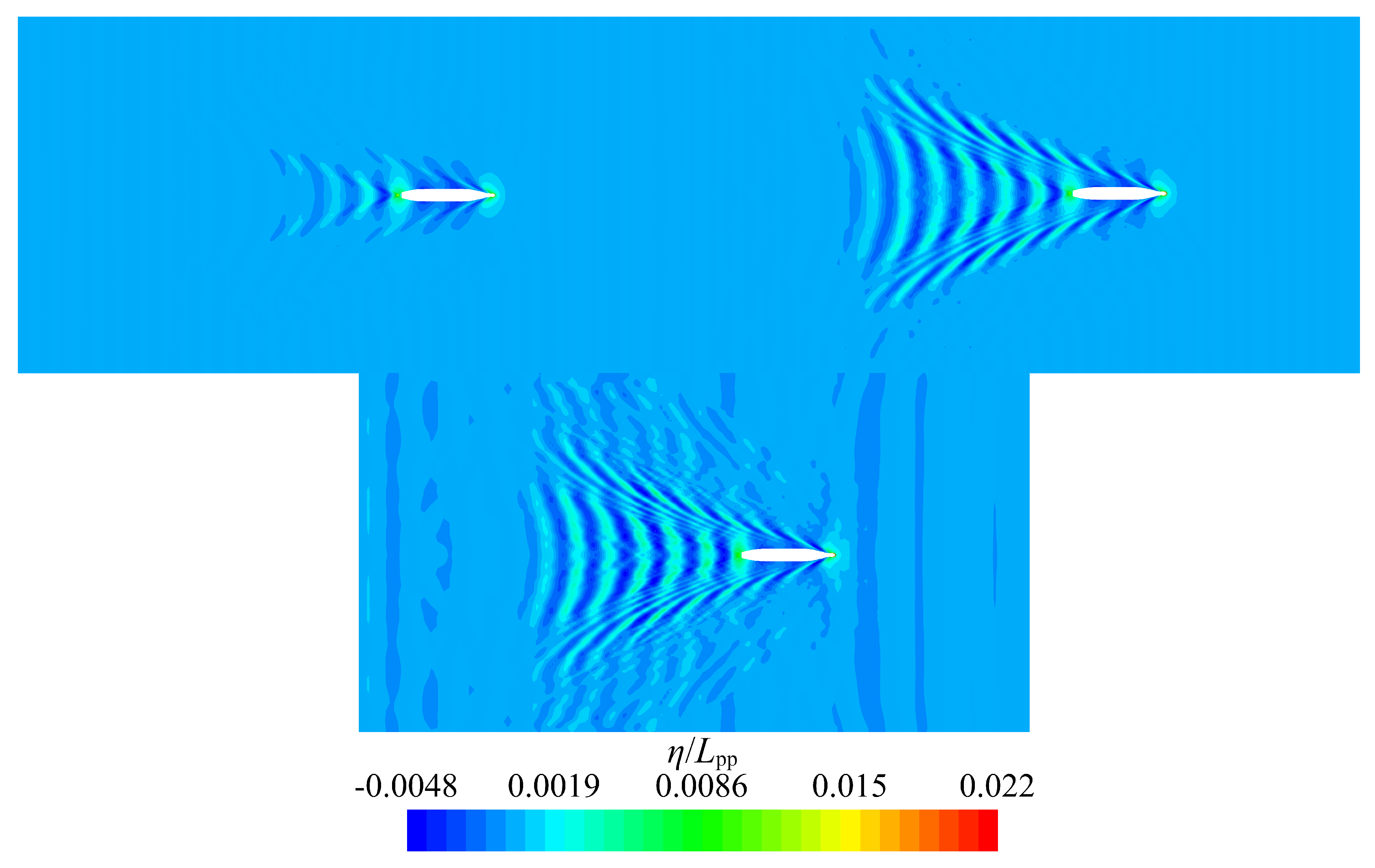
Figure 13.
Wave patterns obtained with first-order (top-left), second-order (top-right) and hybrid third-order (bottom) discretization scheme for convection terms at full scale.
Figure 13.
Wave patterns obtained with first-order (top-left), second-order (top-right) and hybrid third-order (bottom) discretization scheme for convection terms at full scale.
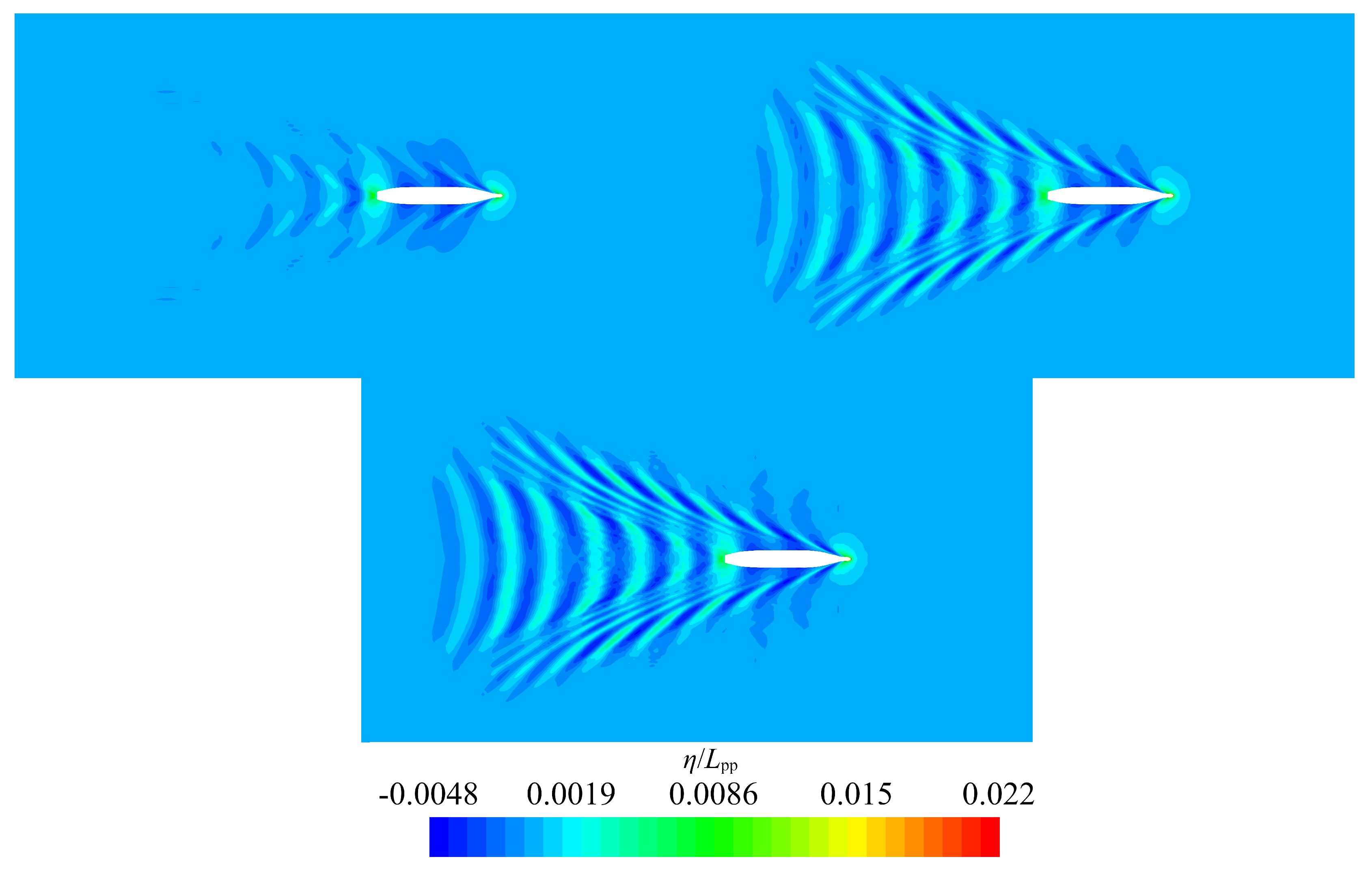
Figure 14.
Wave patterns obtained with first-order (top-left), second-order (top-right) and hybrid third-order (bottom) discretization scheme for convection terms at model scale.
Figure 14.
Wave patterns obtained with first-order (top-left), second-order (top-right) and hybrid third-order (bottom) discretization scheme for convection terms at model scale.
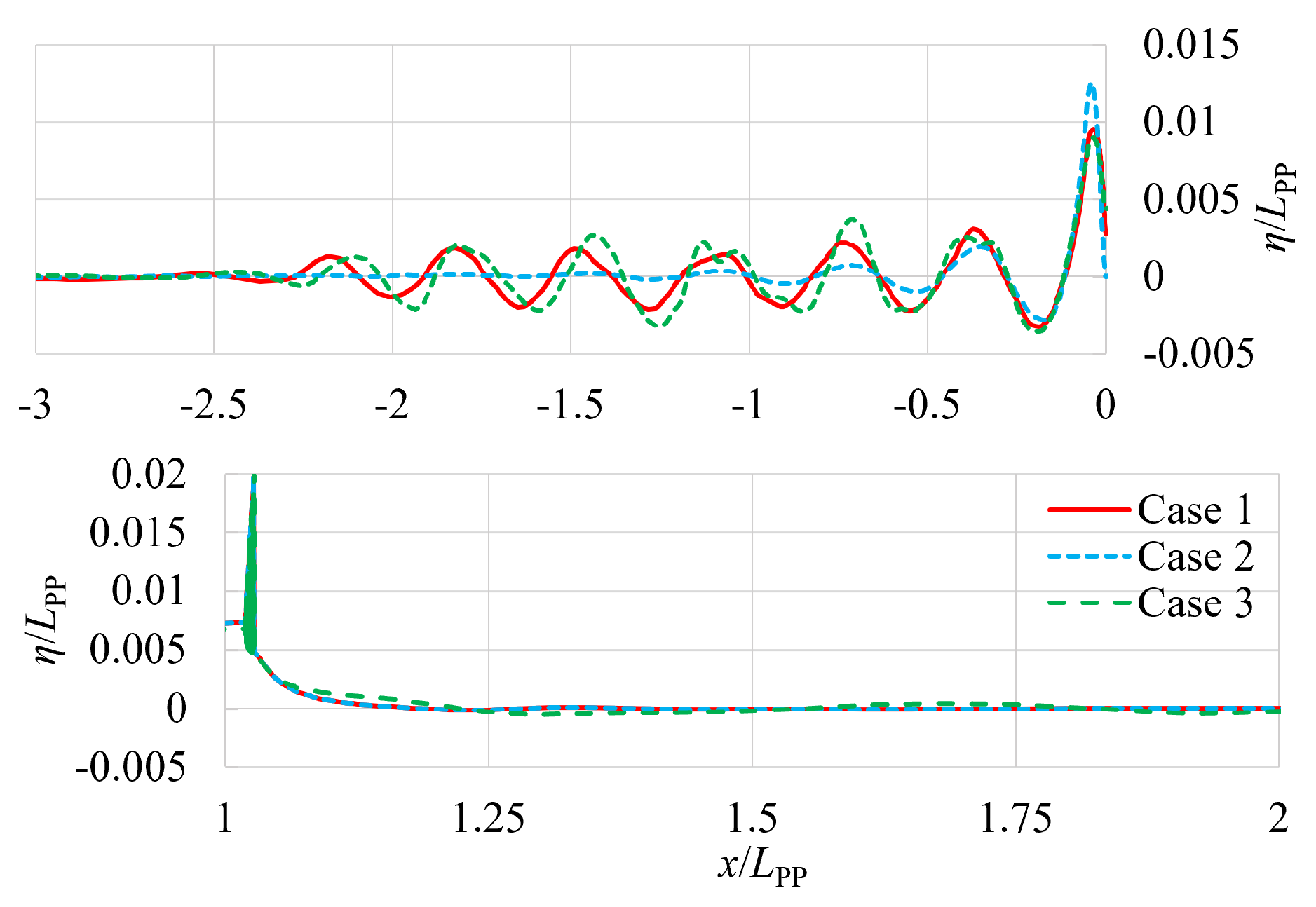
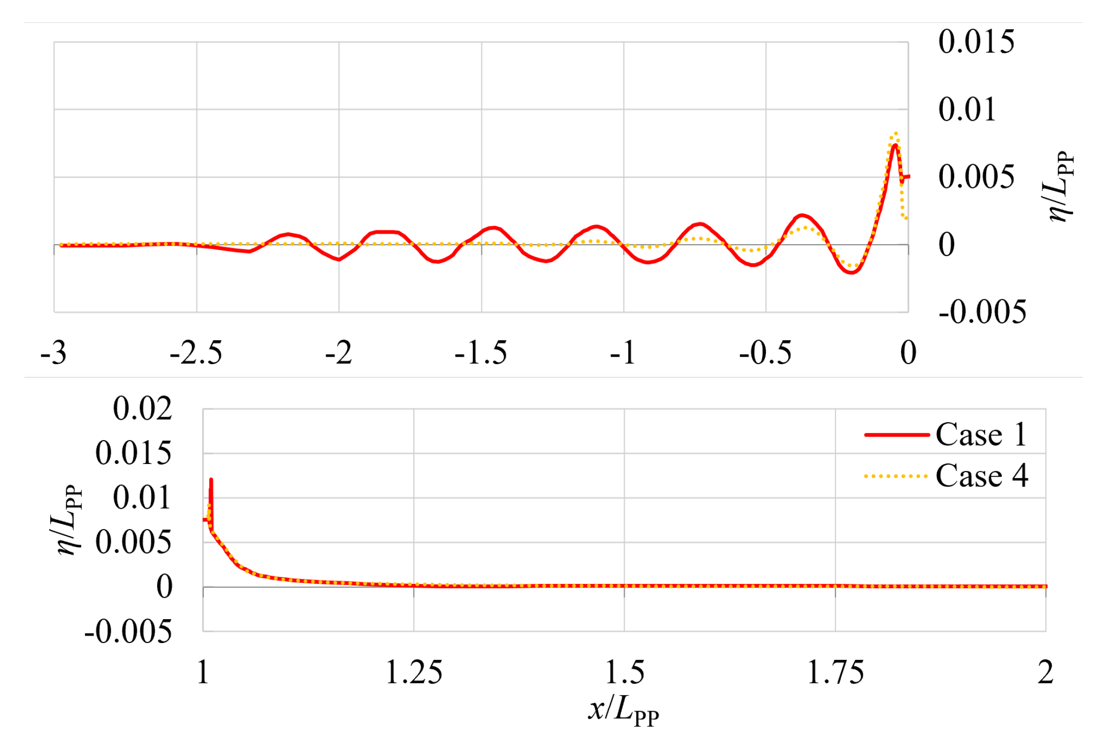
Figure 15.
Wave elevations behind the stern (top) and in front of the ship (bottom), obtained using different discretization schemes for convection terms at full scale.
Figure 15.
Wave elevations behind the stern (top) and in front of the ship (bottom), obtained using different discretization schemes for convection terms at full scale.
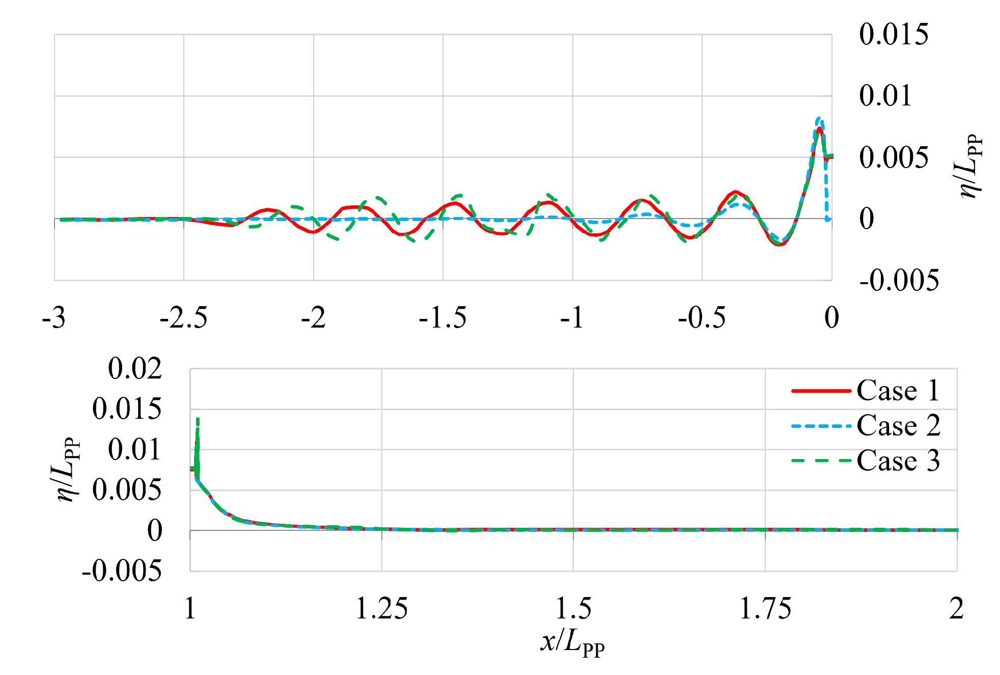
Figure 16.
Wave elevations behind the stern (top) and in front of the ship (bottom), using different discretization schemes for convection terms at model scale.
Figure 16.
Wave elevations behind the stern (top) and in front of the ship (bottom), using different discretization schemes for convection terms at model scale.
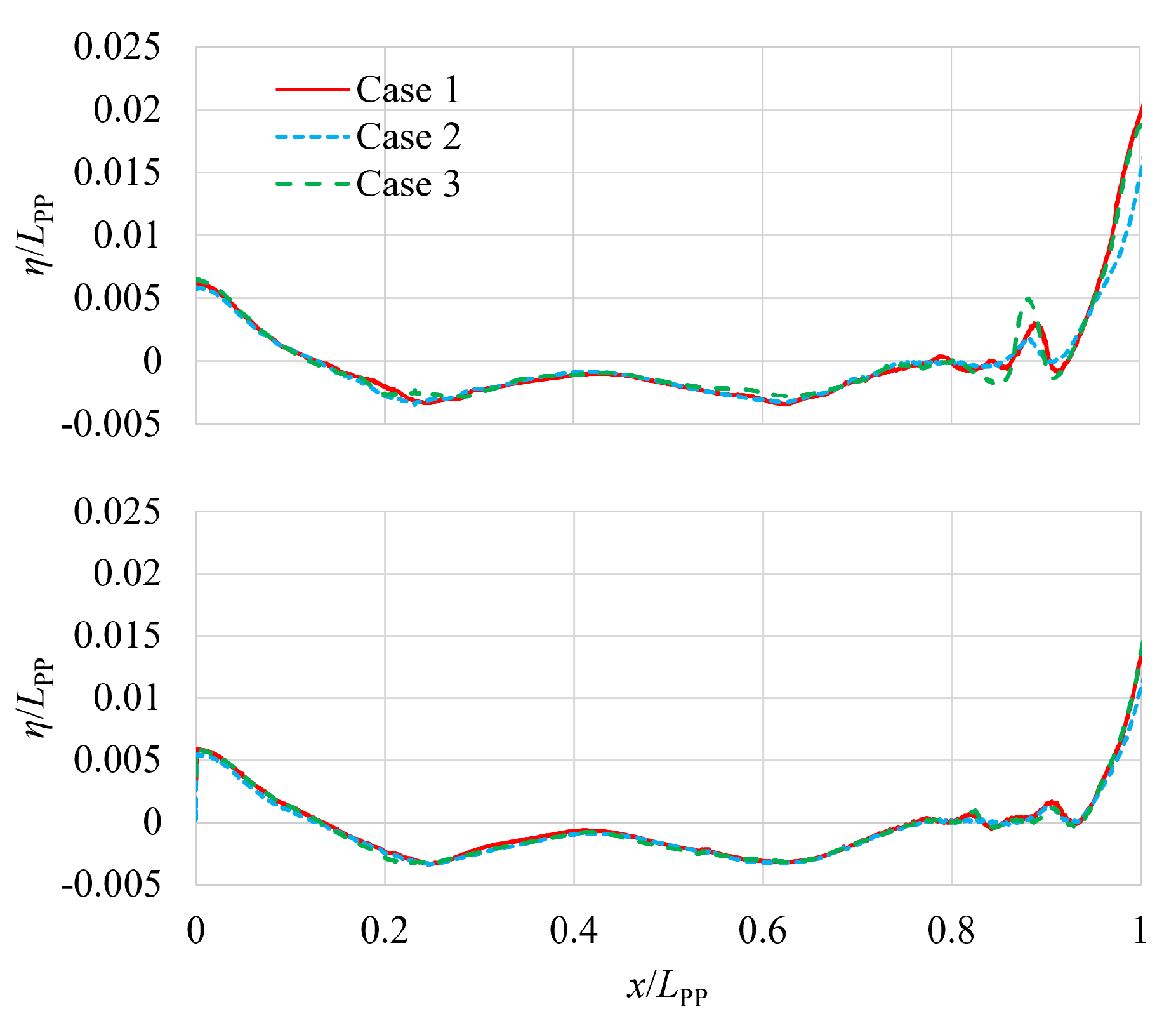
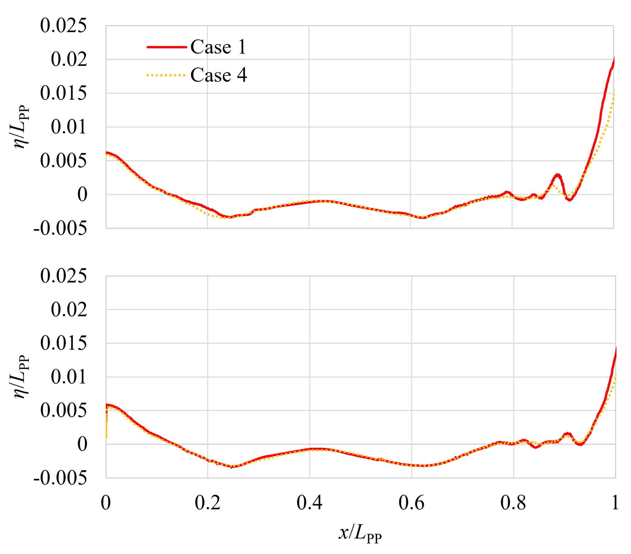
Figure 17.
Wave elevations along the hull at full scale (top) and model scale (bottom) using different discretization schemes for convection terms.
Figure 17.
Wave elevations along the hull at full scale (top) and model scale (bottom) using different discretization schemes for convection terms.
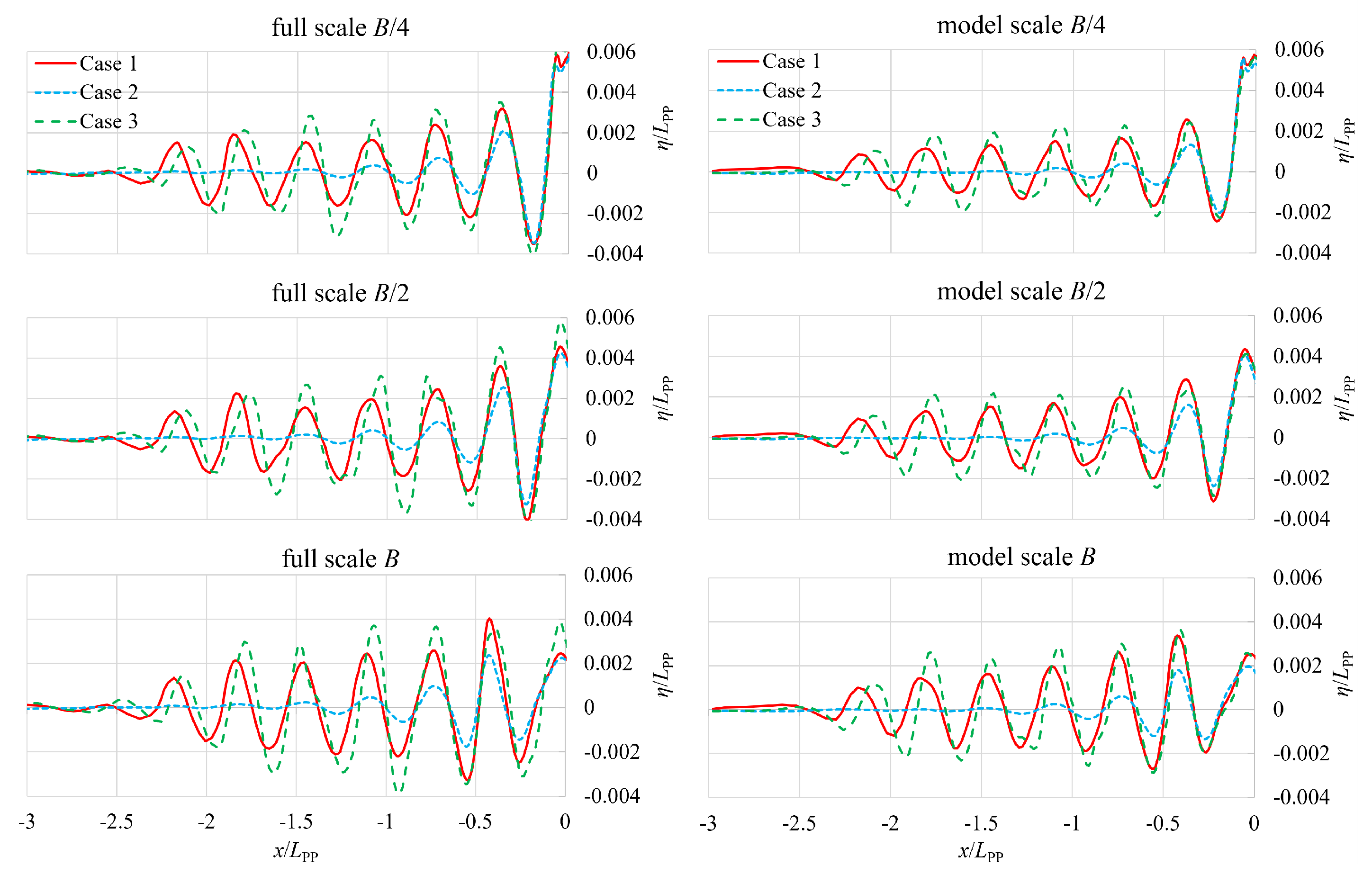
Figure 18.
Wave elevations behind the stern at longitudinal cuts , and B from the centreline of the ship obtained with numerical simulations at full scale (left) and model scale (right).
Figure 18.
Wave elevations behind the stern at longitudinal cuts , and B from the centreline of the ship obtained with numerical simulations at full scale (left) and model scale (right).
Figure 19.
Comparison of two discretization schemes for gradient terms at full scale (left) and model scale (right).
Figure 19.
Comparison of two discretization schemes for gradient terms at full scale (left) and model scale (right).
Figure 20.
Wave elevations behind the stern (top) and in front of the ship (bottom), obtained using the first and second-order scheme for gradient terms at full scale.
Figure 20.
Wave elevations behind the stern (top) and in front of the ship (bottom), obtained using the first and second-order scheme for gradient terms at full scale.
Figure 21.
Wave elevations behind the stern (top) and in front of the ship (bottom), obtained using the first and second-order scheme for gradient terms at model scale.
Figure 21.
Wave elevations behind the stern (top) and in front of the ship (bottom), obtained using the first and second-order scheme for gradient terms at model scale.
Figure 22.
Wave elevations along the hull at full scale (top) and model scale (bottom) using different discretization scheme for gradient terms.
Figure 22.
Wave elevations along the hull at full scale (top) and model scale (bottom) using different discretization scheme for gradient terms.
Figure 23.
Comparison between first-order scheme for convection and gradient terms at full (left) and model scale (right).
Figure 23.
Comparison between first-order scheme for convection and gradient terms at full (left) and model scale (right).
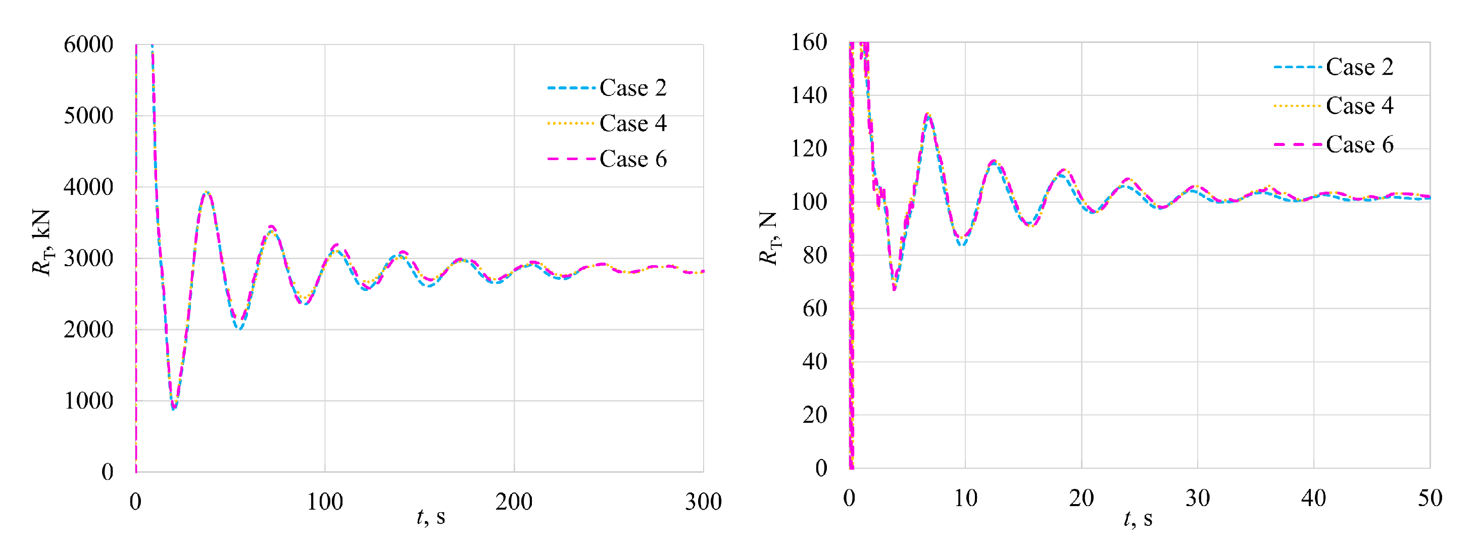
Figure 24.
Comparison between first and second-order discretization scheme for gradient, convection terms and temporal discretization at full scale (left) and model scale (right).
Figure 24.
Comparison between first and second-order discretization scheme for gradient, convection terms and temporal discretization at full scale (left) and model scale (right).
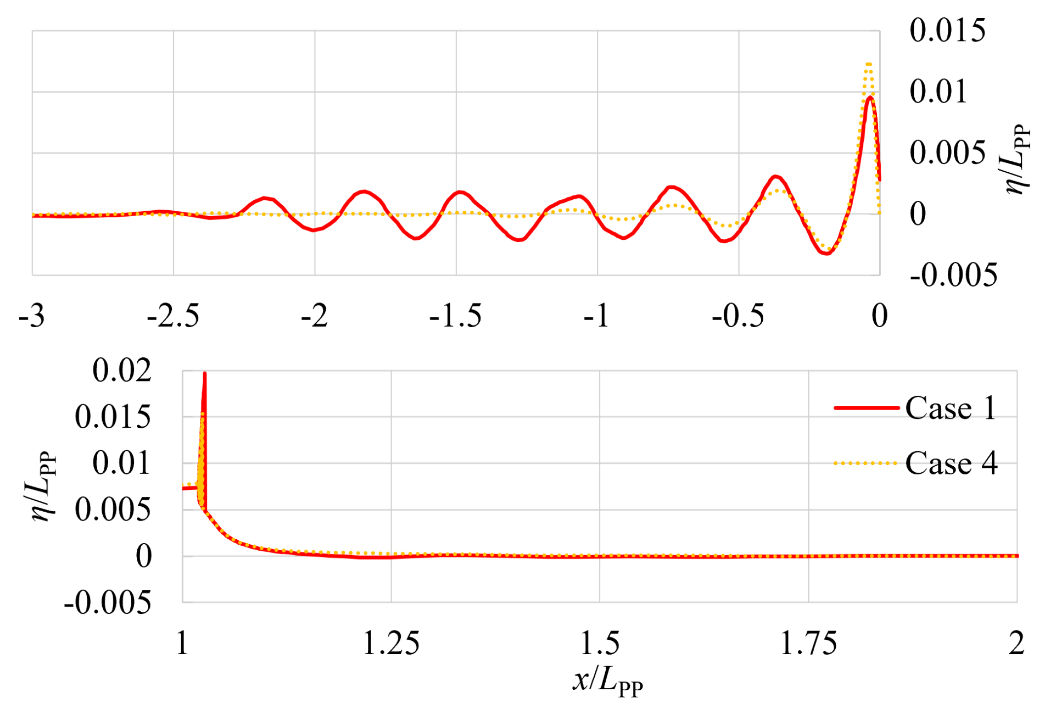
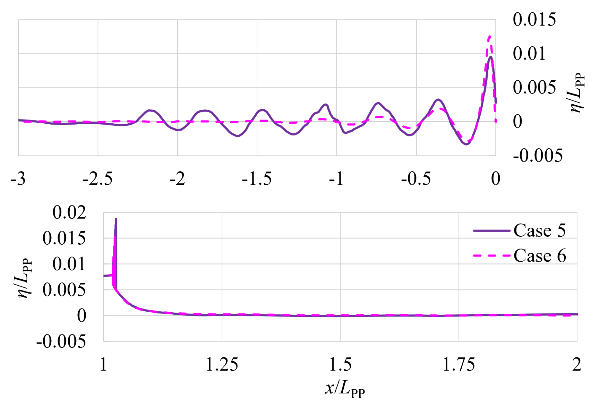
Figure 25.
Wave elevations behind the stern (top) and in front of the ship (bottom), obtained using different discretization schemes for spatial and temporal terms at full scale.
Figure 25.
Wave elevations behind the stern (top) and in front of the ship (bottom), obtained using different discretization schemes for spatial and temporal terms at full scale.
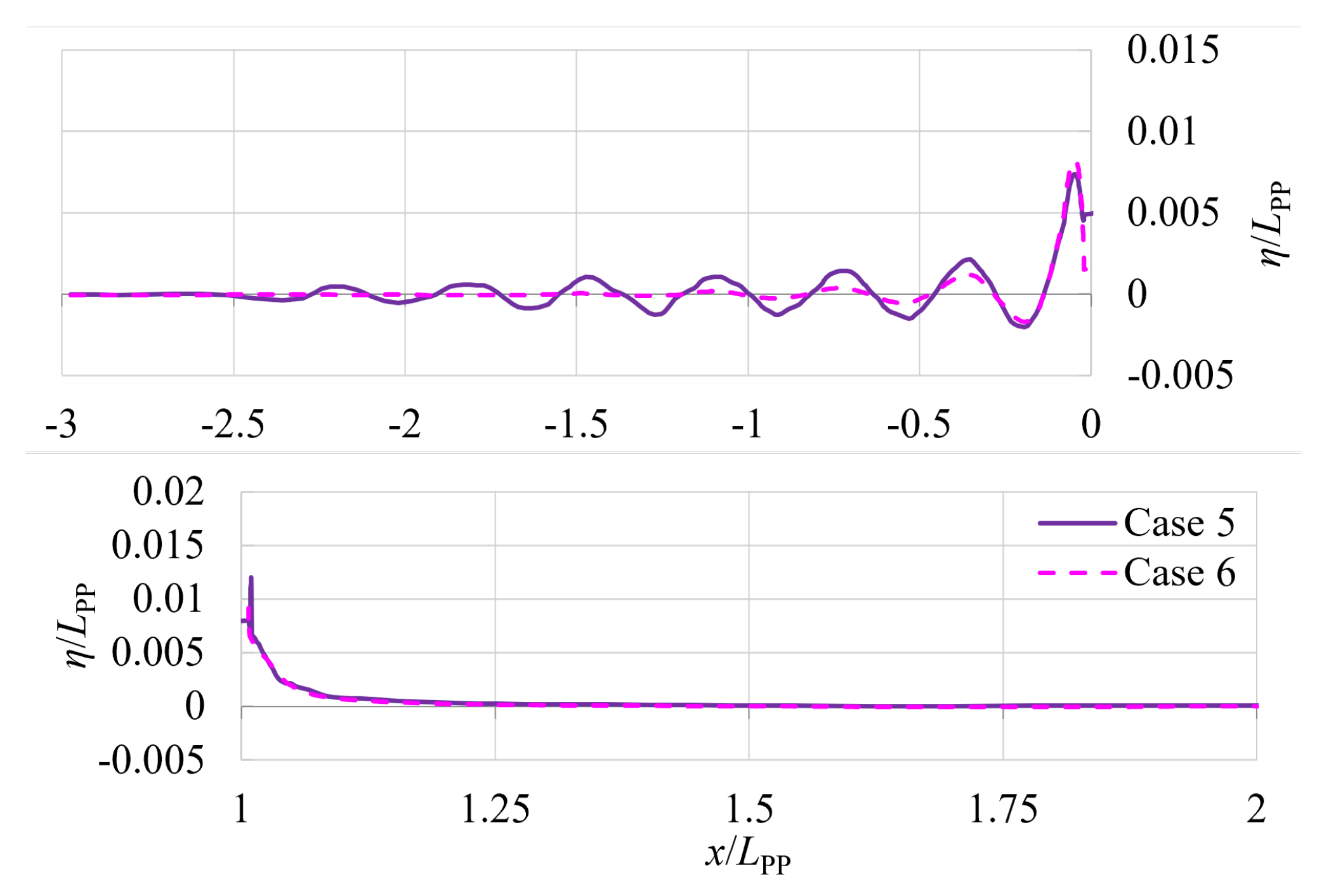
Figure 26.
Wave elevations behind the stern (top) and in front of the ship (bottom), obtained using different discretization schemes for spatial and temporal terms at model scale.
Figure 26.
Wave elevations behind the stern (top) and in front of the ship (bottom), obtained using different discretization schemes for spatial and temporal terms at model scale.
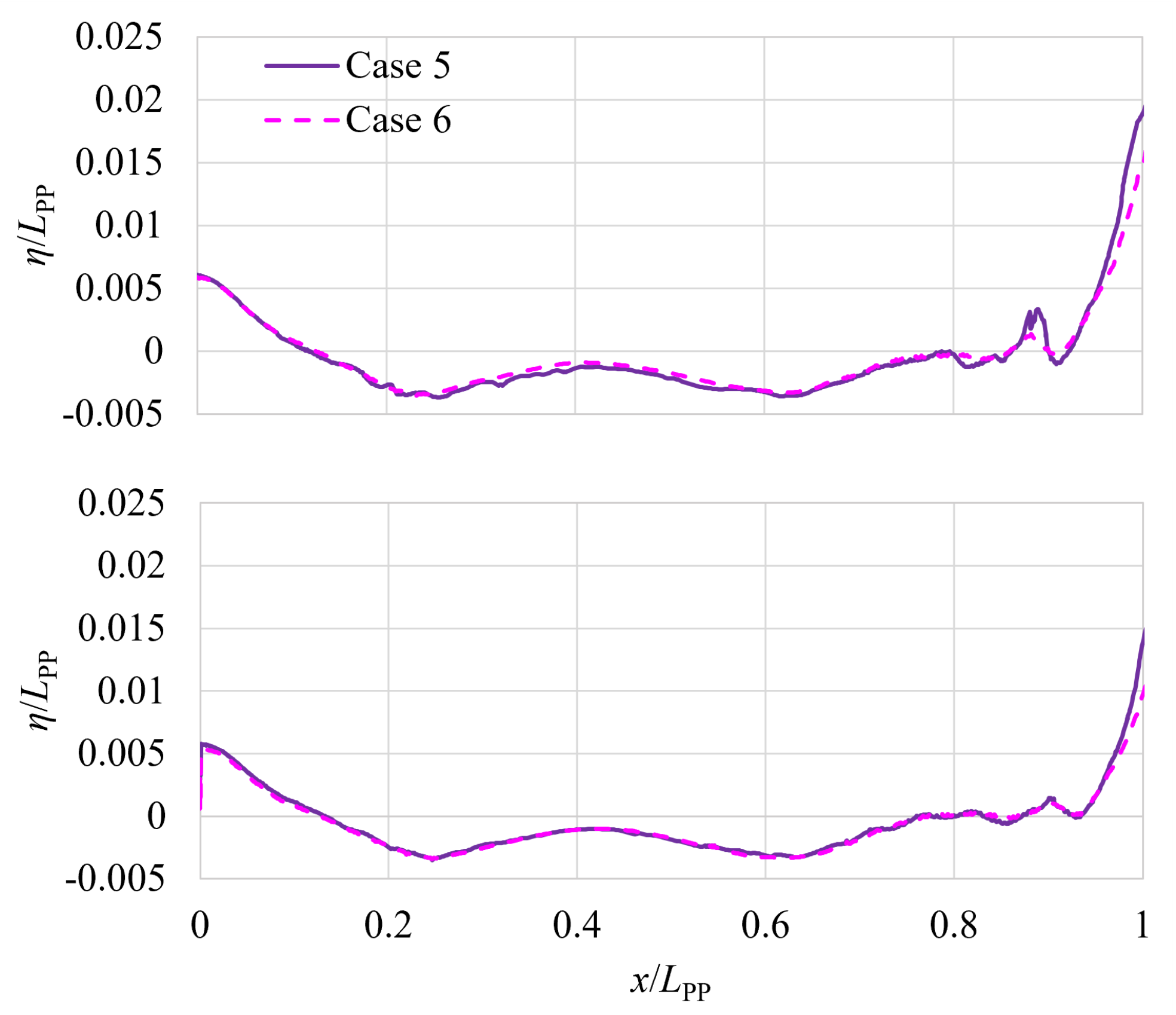
Figure 27.
Wave elevations along the hull at full scale (top) and model scale (bottom) using different discretization schemes for spatial and temporal terms.
Figure 27.
Wave elevations along the hull at full scale (top) and model scale (bottom) using different discretization schemes for spatial and temporal terms.
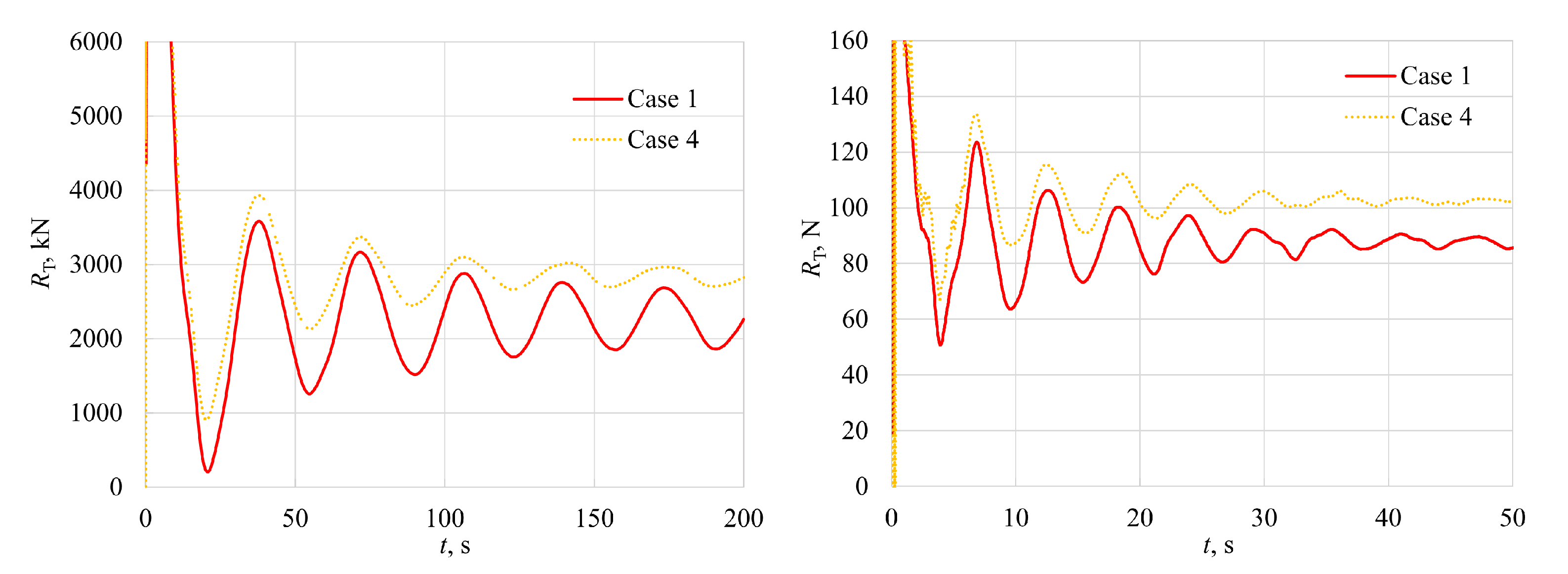
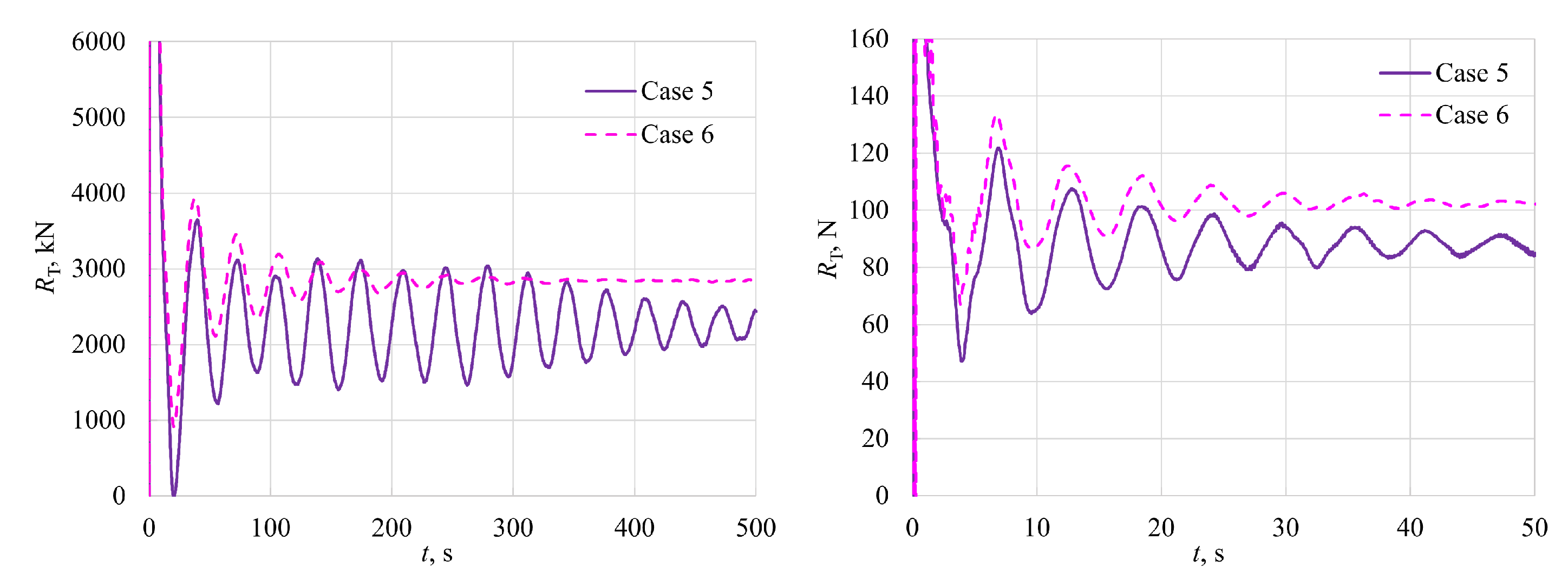
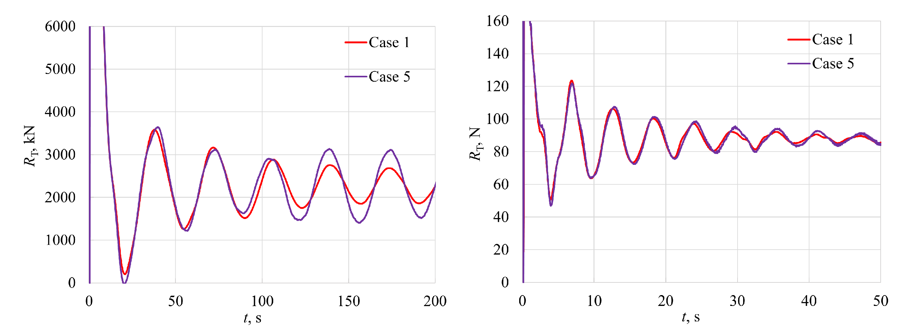
Figure 28.
The impact of the temporal discretization on the total resistance at full scale (left) and model scale (right).
Figure 28.
The impact of the temporal discretization on the total resistance at full scale (left) and model scale (right).
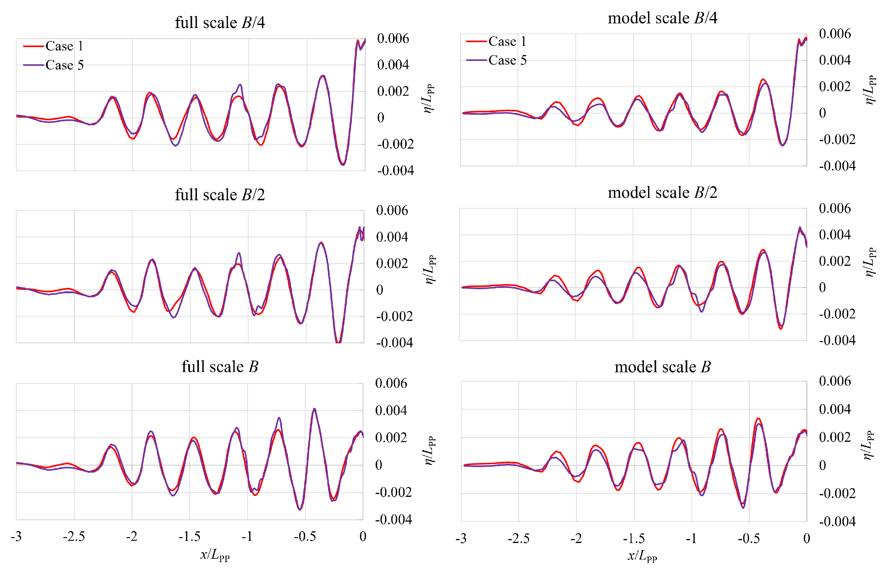
Figure 29.
Wave elevations behind the ship at longitudinal cuts , and B from the centreline of the ship obtained with numerical simulations at full scale (left) and model scale (right).
Figure 29.
Wave elevations behind the ship at longitudinal cuts , and B from the centreline of the ship obtained with numerical simulations at full scale (left) and model scale (right).
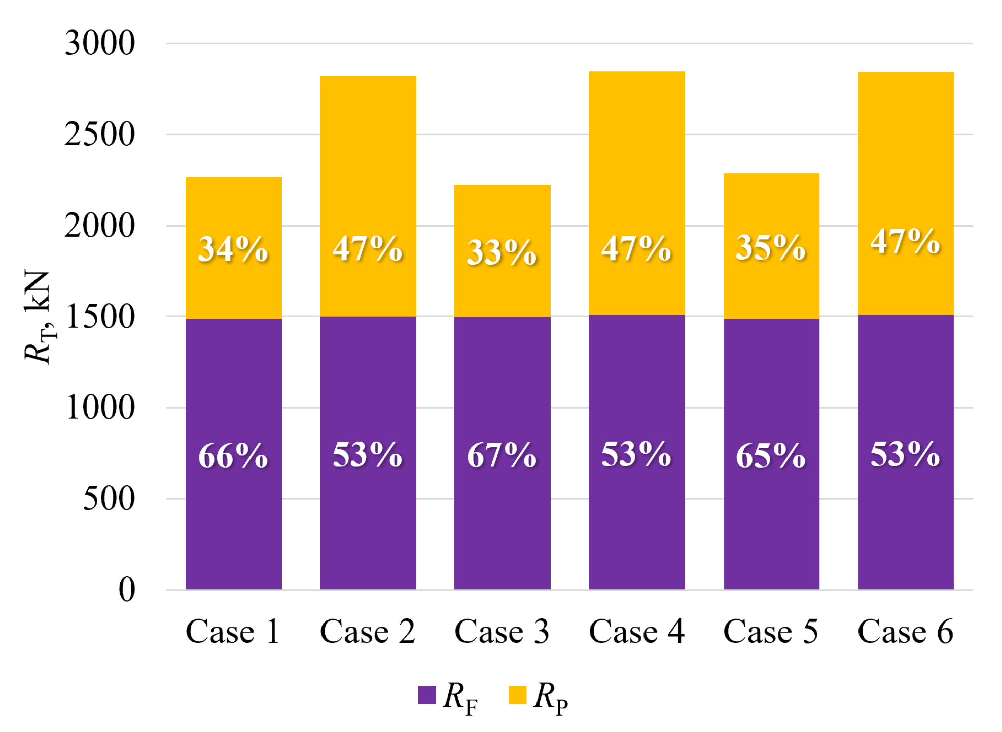
Figure 30.
The portions of the total resistance components obtained with numerical simulations at full scale.
Figure 30.
The portions of the total resistance components obtained with numerical simulations at full scale.
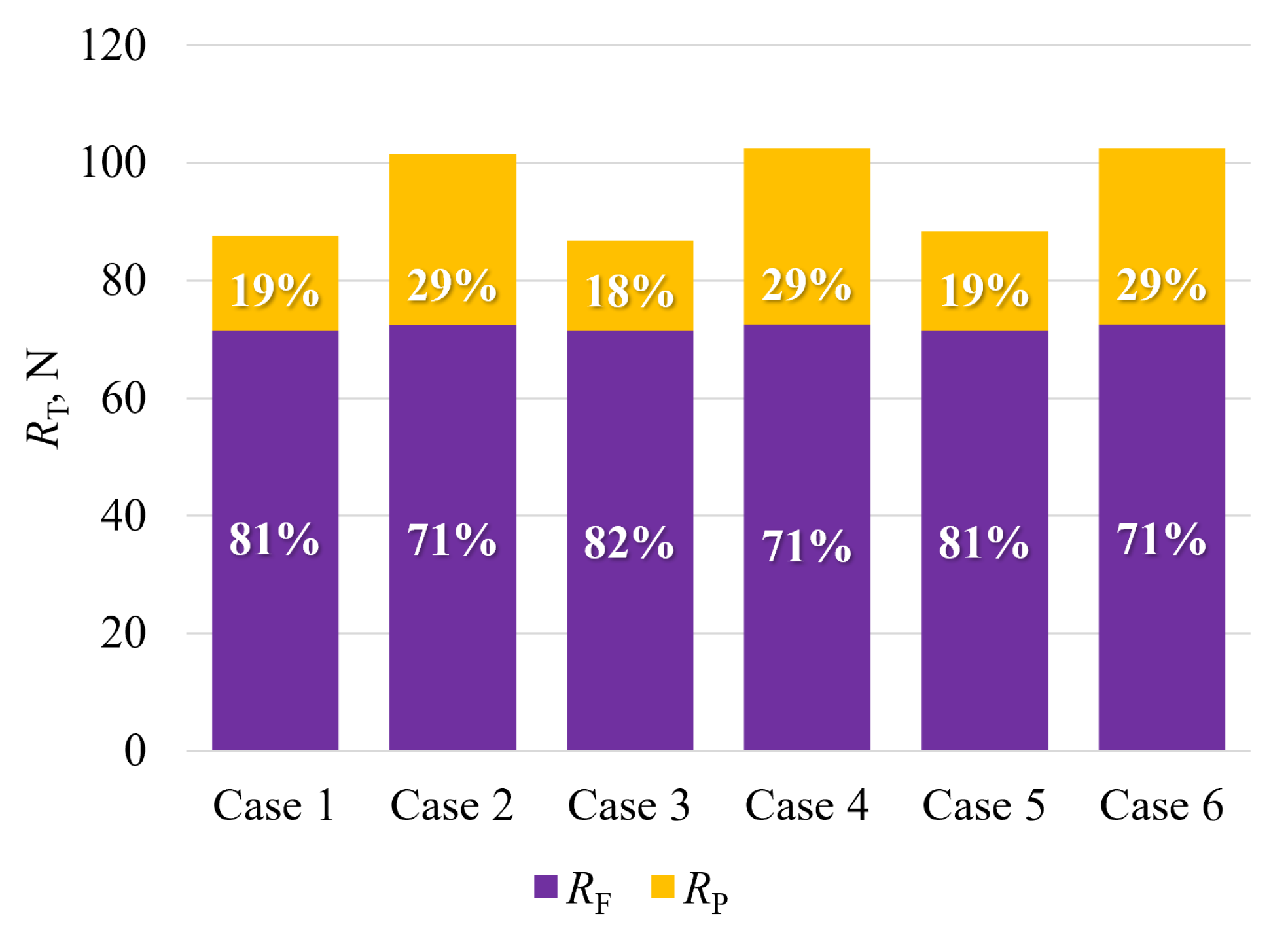
Figure 31.
The portions of the total resistance components obtained with numerical simulations at model scale.
Figure 31.
The portions of the total resistance components obtained with numerical simulations at model scale.
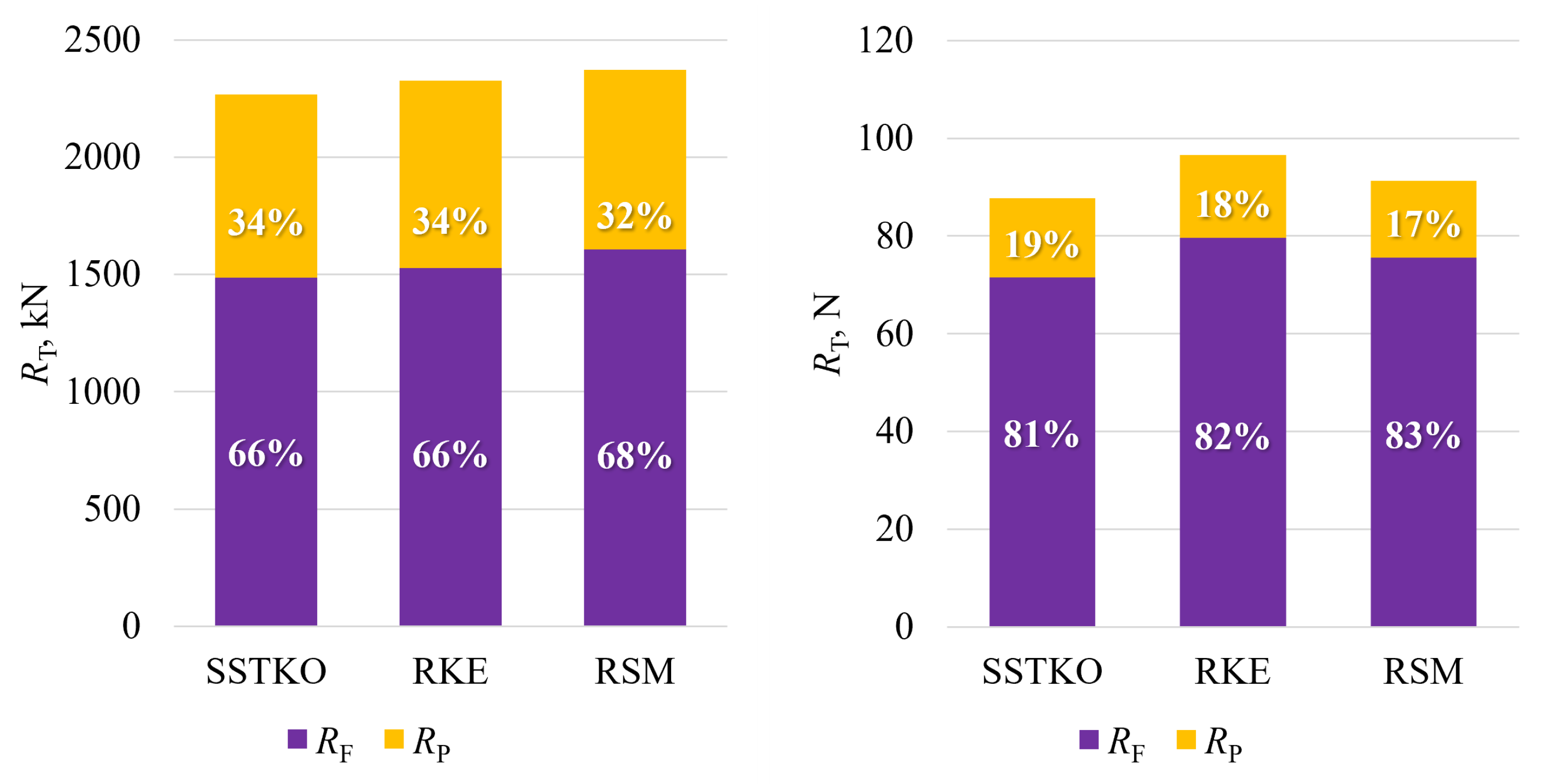
Figure 32.
The portions of the total resistance components obtained with different turbulence models within the numerical simulations at full scale (left) and model scale (right).
Figure 32.
The portions of the total resistance components obtained with different turbulence models within the numerical simulations at full scale (left) and model scale (right).
Table 1.
Post-Panamax 6750-TEU container ship data.
Table 1.
Post-Panamax 6750-TEU container ship data.
| Property | Full Scale | Model Scale |
|---|
| , - | 1 | 35.18 |
| , m | 300.891 | 8.553 |
| , m | 286.6 | 8.147 |
| , m | 281.3 | 7.996 |
| T, m | 11.98 | 0.341 |
| B, m | 40 | 1.137 |
| , t | 85,562.7 | 1.965 |
| , m | 18.662 | 0.531 |
| , m | 2.1 | 0.06 |
| , m | 16.562 | 0.471 |
| , m | 138.395 | 3.934 |
| , m | 14.6 |
| , m | 70.144 |
| , m | 70.144 |
Table 2.
Details of the used grid resolutions.
Table 2.
Details of the used grid resolutions.
| Index | N | |
|---|
| Model Scale | Full Scale | Model Scale | Full Scale |
|---|
| 1 | 2.3 M | 3.7 M | 0.189 | 7.70 |
| 2 | 1.0 M | 2.3 M | 0.248 | 8.99 |
| 3 | 0.4 M | 1.0 M | 0.327 | 11.99 |
Table 3.
Verification study for the time step.
Table 3.
Verification study for the time step.
| Parameter | Model Scale | Full Scale |
|---|
| −7.906 N | 80.524 kN |
| 1.259 N | 31.774 kN |
| 2 | 2 |
| 2 | 2 |
| R | −0.159 | 0.395 |
| p | 2.650 | 1.342 |
| 0.014% | 0.01% |
| 0.003% | 0.01% |
| 0.34% | 1.13% |
Table 4.
Verification study for the grid size.
Table 4.
Verification study for the grid size.
| Parameter | Model Scale | Full Scale |
|---|
| 1.897 N | 80.756 kN |
| −0.013 N | 9.885 kN |
| 1.319 | 1.335 |
| 1.314 | 1.167 |
| R | −0.006 | 0.123 |
| p | 18.142 | 6.228 |
| 0.0001% | 0.44% |
| 0.000001% | 0.27% |
| 0.0001% | 0.34% |
Table 5.
Validation study for the total resistance.
Table 5.
Validation study for the total resistance.
| Turbulence Model | , N | , N | , % |
|---|
| RKE | 96.617 | 94.994 | 1.709 |
| SSTKO | 87.780 | −7.595 |
| RSM | 91.352 | −3.834 |
Table 6.
Total resistance obtained with RKE, SSTKO and RSM turbulence model.
Table 6.
Total resistance obtained with RKE, SSTKO and RSM turbulence model.
| Turbulence Model | , kN | , N |
|---|
| RKE | 2321.11 | 96.62 |
| SSTKO | 2302.87 | 87.73 |
| RSM | 2356.26 | 91.35 |
Table 7.
Different combinations of discretization schemes used in the numerical simulations.
Table 7.
Different combinations of discretization schemes used in the numerical simulations.
| Case | Temporal | Convection | Gradient |
|---|
| 1 | 1st | 2nd | 2nd |
| 2 | 1st | 1st | 2nd |
| 3 | 1st | 3rd | 2nd |
| 4 | 1st | 2nd | 1st |
| 5 | 2nd | 2nd | 2nd |
| 6 | 1st | 1st | 1st |


