Numerical Assessment of the Resistance of a Solar Catamaran in Shallow Water

Abstract

In this paper, a numerical assessment of the effect of shallow water on the total resistance of the solar catamaran SolarCat is carried out using computational fluid dynamics within the software package STAR–CCM+. The unsteady viscous fluid flow was modelled based on the Reynolds-averaged Navier–Stokes (RANS) equations with the application of the $k-\omega$ SST ($k-\omega$ Shear Stress Transport) turbulence model. The RANS equations were discretized by the finite volume method, and the position of the free surface is determined by the volume of fluid method. In shallow water conditions, a mesh morphing algorithm is applied. Numerical simulations were carried out for the deep water and limited depths corresponding to $h/T=7.6$, $h/T=4$, and $h/T=2$ at two speeds. The verification study was carried out and the total numerical uncertainty was calculated for the total resistance and sinkage of the catamaran. A detailed analysis of the flow around the catamaran was carried out.

1. Introduction

In the last few years, the development and raising of environmental awareness have led to the expansion of green technologies aimed at preserving and protecting the environment. The idea of an environmentally friendly and energy-efficient sustainable vessel has resulted in the first solar-electric catamaran for passenger transportation named SolarCat [1]. SolarCat has an integrated solar power plant that derives all the necessary energy from its sources, thus representing a significant technological breakthrough. The use of solar power systems on ships is one of the best ways to utilize green energy as an alternative to fossil fuels [2]. Due to the slower energy conversion of solar panels, solar energy is primarily applied as the main energy source in smaller vessels, while on larger ships it serves as an auxiliary energy source [3]. Furthermore, it has been confirmed that solar-assisted power production on larger vessels can potentially decrease carbon dioxide emissions by up to 12% [4]. Additionally, it has been proven that the use of solar energy meets the greenhouse gas emission requirements for ships according to the recommendations of the International Maritime Organization (IMO) [5]. Sornek et al. [6] highlighted that solar-powered small autonomous surface vehicles for performing water quality measurements can successfully become part of water quality monitoring systems. Low-carbon maritime transport has an important role in the reduction of the greenhouse gas emissions, contributing to a sustainable future. The requirement for technological innovations within the design of zero-emission ships will be a challenge for the maritime industry in the near future [7].

Catamarans that operate at moderate speeds meet the requirements of highly efficient transportation with minimal environmental impact [8]. The increase in fuel prices and the promotion of environmental consciousness have resulted in the development of more energy-efficient catamarans that have greater carrying capacity but operate at lower speeds. The combination of catamaran length and speed transfers the catamaran from the planing regime with dominant tangential stresses to a transitional speed between the displacement and planing regime with tangential and normal stresses of similar magnitude. Improved transverse stability, dependent on the separation of the catamaran demihulls, reduced roll motions in waves compared to monohull vessels, improved seakeeping characteristics in oblique waves, and a smaller draught that enables sailing in shallow water are just some of the advantages of catamarans over monohull vessels [9]. The determination of the multihull configuration is crucial to improve the hydrodynamic performance [10,11], since it has a great influence on the interference resistance [12] Therefore, an investigation of the hydrodynamic characteristics of catamarans is of great interest. When operating in shallow water, the shallow water effect on the total resistance, trim, and sinkage of the catamaran should be taken into account. Ulgen and Dhanak [13] showed that the total resistance coefficient of the catamaran increases by over 40% at transcritical Froude numbers, which are close to the critical value of the Froude number based on water depth.

Scientific interest in the effects of shallow or confined water on ship resistance has existed for a very long time but has become more intense in recent years with growth in ship size and increasing congestion of the shipping routes [14]. The results of the performed numerical calculations for the DTC containership in moderate water depths showed that viscosity affects the ship trim and that the viscous effects become dominant with decreasing under keel clearance [15]. When a ship moves in shallow and restricted water, the flow around the ship hull changes due to the interaction between the hull and the bottom or walls of the waterway [16]. An increase in the flow velocity around the ship hull results in a decrease in the pressure and can lead to maritime accidents such as grounding or stranding. Therefore, to ensure safe navigation, it is crucial to accurately predict the hydrodynamic forces acting on the ship hull, taking into account the influence of shallow water [17]. The increase in the flow velocity around the ship hull is primarily caused by the pressure gradient due to a restricted waterway, leading to an increase in the resistance, draft, and trim of the ship [18]. In shallow water, the pressure on the midship part of a hull decreases, while the pressure on the bow and stern increases. Consequently, the water level rises at the bow and stern and decreases at the midship part of the ship. The occurrence of a squat in shallow water at high speeds can result in grounding if the under-keel clearance is insufficient [19].

Given the importance of water depth and ship speed, the Froude number based on depth $F{r}_h=v/\sqrt{gh}$ is defined representing the ratio of the ship speed to the critical speed of the wave propagation in shallow water [20]. The critical ship speed is determined based on the $F{r}_h$. When $F{r}_h<1$, the ship speed is called subcritical, while for $F{r}_h>1$ the speed is supercritical. In the case of subcritical speed, the increase in both bow and stern drafts is greater compared to their difference [21]. The three main parameters affecting the ship squat are the blockage factor, the block coefficient, and the ship speed [22]. The blockage factor is the ratio of the submerged midship cross-sectional area and the underwater area of the canal or channel.

According to Schlichting’s research on the effects of shallow water, a decrease in the ship speed in shallow water is determined based on the assumption that the wave resistance in shallow water is the same as the one in deep water [14]. Maintaining the same speed in shallow water as in deep water results in increased resistance, draft, and trim of the ship, which can lead to grounding [23]. Shallow water affects wave resistance through changes in the wave pattern depending on $F{r}_h$. In general, the value of the wave resistance coefficient significantly increases when $F{r}_h$ reaches the critical value ($F{r}_h=1$), but it rapidly decreases with a further increase in $F{r}_h$ [24]. The importance of predicting the ship behavior in shallow and confined waters is multiple [25]; it contributes to the decision-making when it comes to the channels’ dredging, influences the safe levels of the sea state and ship speed prescribed by the port authorities, and enables the creation of adequate mathematical models for ship maneuvering in shallow waters which are then implemented in bridge simulators and navigators. Lataire et al. [26] proposed a new mathematical model for the determination of the ship sinkage by taking into account the forward speed, propeller action, lateral position in the fairway, total width of the fairway, and water depth. The new model is based on the results of the performed model tests for large crude carrier in canals of different widths.

There are various approaches to predicting ship resistance in shallow water, including empirical or analytical expressions, numerical calculations, and experiments. Analytical methods mostly rely on assumptions of potential flow theory, considering the ship as a slender body. Tuck [27] proposed formulae for the prediction of the wave resistance and vertical forces of a ship sailing at subcritical and supercritical speeds at limited depths based on the slender body theory. Based on the vertical forces sinkage and trim can be obtained. The proposed formulae were further extended to include the effects of limited width on the ship as well [28]. Gourlay [29] proposed a general Fourier transform method for the determination of the ship squat in open water, a rectangular canal, a dredged channel, a stepped canal, or a channel of arbitrary cross-section. As an extension to Schlichtings’s method, Lackenby [30] proposed a diagram for the estimation of the shallow water effects, i.e., speed loss under the incipient shallow water conditions.

Empirical expressions have certain limitations and conditions that need to be satisfied when applied. Furthermore, effects that are neglected in potential theory, such as wave breaking, turbulence, and viscosity, are significant in shallow water and should be considered. Reynolds-averaged Navier–Stokes (RANS) equations provide a good alternative to potential flow theory as they consider the viscous effects of fluid flow [31]. Numerical tools based on RANS equations have proven to be highly effective in determining the total resistance and resistance components of catamarans operating at moderate speeds [8]. The combination of experimental and Computational Fluid Dynamics (CFD) currently represents the best practice for the investigation of hydrodynamic characteristics. For example, by performing the experimental and numerical investigations of the influence of the lateral separations on the maneuvering performance of a small waterplane area twin hull, Dai and Li [32] showed that turning performance decreased for the intermediate demihull separation, while the demihull separation showed little impact on zigzag maneuver. CFD allows for accurate prediction of the draft, trim, and ship resistance in shallow water [22], and, as such, it can serve as an alternative to expensive and time-consuming experimental tests in towing tanks that are capable of performing tests in shallow and restricted water.

The rest of the paper is organized as follows: in Section 2 the case study is given. Section 3 describes the mathematical model, and the numerical setup is summarized in Section 4. The obtained numerical results, along with the discussion, are given in Section 5 followed by the conclusions in Section 6.

2. Case Study

The numerical simulations of the resistance test in deep and shallow water were conducted for the solar catamaran with main particulars given in

Table 1. Main particulars of the solar catamaran.

Main Particular	Symbol	Value
Length between perpendiculars	$L_{PP}$	15 m
Breadth	$B$	5 m
Demihull breadth	$b$	1.59 m
Draught	$T$	0.68 m
Displacement mass	$\Delta$	15.45 t
Vertical position of the center of gravity	$KG$	1.78 m
Longitudinal position of the center of gravity	$LCG$	6.88 m

[1]. The influence of shallow water on the total resistance, sinkage, and trim was assessed.

A 3D model of the catamaran is shown in Figure 1. The coordinate system is located at the symmetry plane of the catamaran at the center of gravity according to Table 1. The positive direction of the $x$-axis is oriented towards the bow, the $y$-axis towards the port side, and the $z$-axis upwards. Accordingly, the sinkage of the catamaran represents a displacement in the negative direction of the $z$-axis, the negative trim angle represents bow down, and the positive trim angle bow up.

3. Mathematical Model

Reynolds-averaged Navier–Stokes equations along with the continuity equation are used to describe the unsteady incompressible turbulent flow:

$$\frac{\partial \left(\rho {\overline{u}}_i\right)}{\partial t}+\frac{\partial }{\partial x_j}\left(\rho {\overline{u}}_i{\overline{u}}_j+\rho \overline{{u^{\prime }}_i{u^{\prime }}_j}\right)=-\frac{\partial \overline{p}}{\partial x_i}+\frac{\partial {\overline{\tau }}_{ij}}{\partial x_j}$$

(1)

$$\frac{\partial \left(\rho {\overline{u}}_i\right)}{\partial x_i}=0$$

(2)

where $\rho$ is the fluid density, ${\overline{u}}_i$ is the averaged Cartesian components of the velocity vector, $\rho \overline{{u^{\prime }}_i{u^{\prime }}_j}$ is the Reynolds stress tensor, and $\overline{p}$ is the mean pressure. The mean viscous stress tensor is defined as:

$${\overline{\tau }}_{ij}=\mu \left(\frac{\partial {\overline{u}}_i}{\partial x_j}+\frac{\partial {\overline{u}}_j}{\partial x_i}\right)$$

(3)

where $\mu$ is the dynamic viscosity.

Within this study, the $k-\omega \hspace{0.17em}\mathrm{SST}$ turbulence model was applied for the closure of Equations (1) and (2), which incorporates two additional transport equations, one for the specific kinetic energy and one for the specific dissipation rate [33].

4. Numerical Setup

The governing equations are discretized using the finite volume method and solved in a segregated manner. The convection terms in RANS equations are discretized using second-order upwind scheme, while for temporal discretization, the first-order temporal scheme is used. To track and locate the free surface the Volume of Fluid (VOF) method is utilized combined with the High-Resolution Interface Capturing (HRIC) scheme.

4.1. Computational Domain and Boundary Conditions

Since the catamaran is symmetric, only half of the computational domain is discretized. The boundaries of the computational domain for the numerical simulations in deep water were set as follows. The inlet and top boundaries were placed $1.5L_{PP}$ away from the hull. The outlet boundary was placed $3L_{PP}$ behind the hull, the bottom boundary $2.5L_{PP}$ below the hull, and the side boundary $2L_{PP}$ from the symmetry plane of the catamaran. In numerical simulations for limited water depth, the bottom boundary of the computational domain was placed according to the $h/T$ ratio as $0.3L_{PP}$, $0.14L_{PP}$, and $0.05L_{PP}$ below the keel line for $h/T=7.6$, $h/T=4$, and $h/T=2$, respectively.

It should be noted that the water depth to draught ratio $h/T=7.6$ corresponds to the water depth without the shallow water effect on a ship, which is calculated as follows [34]:

$$\frac{h}{T}\ge 4+3F{r}_T^3$$

(4)

where $F{r}_T^{}=\frac{v}{\sqrt{gT}}$ is the Froude number calculated based on the draught.

The velocity inlet boundary condition was set at the inlet, top, and bottom boundaries of the computational domain for the numerical simulations in deep water. At the outlet boundary, the pressure outlet boundary condition was set, while the symmetry boundary condition was defined at the symmetry plane of the catamaran. The no-slip wall boundary condition was defined for the catamaran hull. In the case of limited depth, a no-slip wall boundary condition was also applied at the bottom with a relative velocity equal to the catamaran speed in the opposite direction [23]. The overview of boundary conditions for deep and limited water depths is given in Figure 2 and Figure 3, respectively.

4.2. Discretization of the Computational Domain

When using CFD tools, the number of cells in the generated mesh has a significant impact on the obtained numerical results, and a compromise needs to be made between the required simulation time and result accuracy [35,36].

To resolve the flow in the areas of interest, the mesh was additionally refined where the free surface was expected, to capture the Kelvin wake around the catamaran demihull, in the area between the catamaran demihulls, as well as between the demihull and bottom within the numerical simulations for limited water depth. In the case of limited water depth, the boundary layer forms at the bottom, and, therefore, the area near the bottom needs to be further refined with prism cells. Since the height of the first cell in the boundary layer depends on the Reynolds number, to ensure the desired value of the non-dimensional distance from the wall ($y^{+}$) the discretization parameters for the boundary layer are adjusted for each speed. The discretization of the boundary layer along the catamaran hull and near the bottom of the computational domain for $h/T=7.6$ at the speed of 5.5 knots is presented in Figure 4.

Based on the International Towing Tank Conference (ITTC) recommendations, the value of the parameter $y^{+}$ should be larger than 30 to describe the flow with a logarithmic velocity profile [37]. To resolve the flow in the boundary layer around the catamaran, wall functions were applied, while on the bottom of the computational domain, the value of the $y^{+}$ parameter was kept below 1. Values of the $y^{+}$ parameter along the catamaran demihull in deep water at the speed of 5.5 knots are shown in Figure 5, and it can be seen that the $y^{+}$ is in the range $30<y^{+}<300$.

As already mentioned, to obtain the wave pattern around the catamaran, it is necessary to refine the region in which the free surface is expected, Figure 6 and Figure 7. It should be noted that the cross-section of the mesh given in Figure 6 corresponds to $h/T=2$.

The number of cells of the mesh used in the numerical simulations at a speed of 5.5 knots can be seen in

Table 2. The number of cells of the mesh used in the numerical simulations at a speed equal to 5.5 knots.

Water Depth	Number of Cells
$h/T\to \infty$	3,488,816
$h/T=7.6$	4,187,987
$h/T=4$	4,234,076
$h/T=2$	4,419,462

.

4.3. The Verification Study

The verification study enables the estimation of the numerical uncertainty of the obtained numerical results. The total numerical uncertainty $U_{SN}$ is defined based on the number of iterations ${\delta }_I$, grid size ${\delta }_G$, time step ${\delta }_T$, and other parameters ${\delta }_P$, and is given as follows [38]:

$$U^2{}_{SN}=U_I^2+U_G^2+U_T^2+U_P^2$$

(5)

where $U_I$ is the numerical uncertainty of the number of iterations, $U_G$ is the numerical uncertainty of the grid size, $U_T$ is the numerical uncertainty of the time step, and $U_P$ is the numerical uncertainty of other parameters.

Within this study, the numerical uncertainty of the grid size and time step was assessed for the total resistance and sinkage of the catamaran in both deep and shallow water using the GCI method [39]. The numerical uncertainty arising from the number of iterations and other parameters can be neglected.

To carry out a convergence study, a minimum of three solutions is required to determine the convergence ratio, which is based on the differences between solutions obtained using different grid sizes and time steps:

$${\epsilon }_{ij}={\varphi }_i-{\varphi }_j$$

(6)

$$R={\epsilon }_{21}/{\epsilon }_{32}$$

(7)

where $\varphi$ is the solution, ${\epsilon }_{ij}$ is the difference between the obtained results, and $R$ is the convergence ratio.

The convergence types based on the convergence ration are given in

Table 3. Convergence types.

Convergence Ratio	Convergence Type
$-1<R_i<0$	Oscillatory
$0<R_i<1$	Monotonic
$\left|R_i\right|>1$	Divergence

.

Within the GCI method, the apparent order of the method can be calculated as follows:

$$p=\frac{1}{\ln r_{21}}\cdot \left|\ln \left|\frac{{\epsilon }_{32}}{{\epsilon }_{21}}\right|+q(p)\right|$$

(8)

where $q(p)$ can be determined as:

$$q(p)=\ln \left(\frac{r_{21}^p-s}{r_{32}^p-s}\right)$$

(9)

$$s=1\cdot \mathrm{sgn}\left(\frac{{\epsilon }_{32}}{{\epsilon }_{21}}\right)$$

(10)

where $r$ is the refinement ratio, which is $\sqrt{2}$ for the grid size, and 2 for the time step [38]. The apparent order of the method $p$ is calculated by solving the Equations (8)–(10) iteratively. Extrapolated values and the approximate and extrapolated relative errors are calculated as follows:

$${\varphi }_{\mathrm{ext}}^{21}=\frac{r_{21}^p{\varphi }_1-{\varphi }_2}{r_{21}^p-1}$$

(11)

$$e_{\mathrm{a}}^{21}=\left|\frac{{\varphi }_1-{\varphi }_2}{{\varphi }_1}\right|$$

(12)

$$e_{\mathrm{ext}}^{21}=\left|\frac{{\varphi }_{\mathrm{ext}}^{21}-{\varphi }_1}{{\varphi }_{\mathrm{ext}}^{21}}\right|$$

(13)

The GCI for fine grid can be calculated with following equation:

$$GC{I}_{\mathrm{fine}}^{21}=\frac{1.25\hspace{0.17em}{e}_{\mathrm{a}}^{21}}{r_{21}^p-1}$$

(14)

According to [40], GCI for coarser grid can be calculated as:

$$GC{I}_{\mathrm{medium}}^{32}=r_{21}^{p}GC{I}_{\mathrm{fine}}^{21}$$

(15)

4.4. Physical Model of the Numerical Simulations and Solver Parameters

Two fluid phases are defined based on the Eulerian Multiphase model, and the initial position of the free surface, as well as the fluid velocity, is defined based on the VOF approach. To prevent wave reflections against the boundaries of the computational domain, the damping layer approach was used with a constant value of damping length equal to the length of the catamaran. The damping layer was applied at the inlet, side, and outlet boundaries. The Dynamic Fluid Body Interaction (DFBI) model was enabled to calculate the sinkage and trim, i.e., within the DFBI model, heave and pitch motion of the catamaran are enabled. To accommodate possibly more pronounced sinkage and trim values within the numerical simulations for limited depth, mesh morphing was applied based on the BSpline algorithm [41,42]. The time step is defined based on the following expression:

$$\Delta t=\frac{T}{c}$$

(16)

where $T$ is the period defined as:

$$T=\frac{L_{PP}}{v}$$

(17)

where $v$ is the ship speed in m/s. The coefficient $c$ for the fine time step was equal to 200, for the medium time step to 100, and for the coarse time step to 50. Therefore, the fine, medium, and coarse time step was equal to 0.01325 s, 0.0265 s, and 0.053 s, respectively. The under-relaxation factors for velocity and pressure were set as 0.7 for the velocity and 0.4 for the pressure. The number of inner iterations was equal to 5.

5. Results and Discussion

Within this section, the obtained results of numerical simulations of the resistance test for the catamaran in deep and shallow water are presented, along with the results of the performed verification study. The results of the validation study for the Series 60 catamaran for a wide range of Froude numbers can be found in [12]. The numerical uncertainty is determined for the total resistance and sinkage of the catamaran at the speed of 5.5 knots in deep water and for $h/T=2$. The free surface, wave patterns, distribution of hydrodynamic pressure along the catamaran hull, pressure distribution on the bottom of the computational domain, tangential stresses, velocity field in the symmetry plane, and wave elevations are shown. Additionally, a comparison of the obtained results for the total resistance, trim, and sinkage for all investigated depths and speeds is provided.

5.1. The Results of the Verification Study

The verification study was performed for the obtained numerical results in deep and shallow water with $h/T=2$ at the speed of 5.5 knots. To assess the numerical uncertainty of the grid size, the numerical simulations were conducted using fine, medium, and coarse mesh with the medium time step. The uncertainty of the time step was determined by performing the numerical simulations with medium mesh using three different time steps. The results of the performed verification study for the numerical simulations in deep water are given in

Table 4. The numerical uncertainty of the grid size for the total resistance in deep water.

${\mathit{\epsilon }}_{21}, \mathbf{N}$	${\mathit{\epsilon }}_{32}, \mathbf{N}$	$\mathit{R}$	$\mathit{p}$	${\mathit{e}}_{\mathbf{a}}^{21},\mathit{\%}$	${\mathit{e}}_{\mathbf{ext}}^{21},\mathit{\%}$	$\mathit{G}\mathit{C}{\mathit{I}}_{\mathbf{fine}}^{21},\mathit{\%}$	$\mathit{G}\mathit{C}{\mathit{I}}_{\mathbf{medium}}^{32},\mathit{\%}$
−2.79	−4.67	0.5974	1.4863	0.004	0.0059	0.74	1.24

and

Table 5. The numerical uncertainty of the time step for the total resistance in deep water.

${\mathit{\epsilon }}_{21}, \mathbf{N}$	${\mathit{\epsilon }}_{32}, \mathbf{N}$	$\mathit{R}$	$\mathit{p}$	${\mathit{e}}_{\mathbf{a}}^{21},\mathit{\%}$	${\mathit{e}}_{\mathbf{ext}}^{21},\mathit{\%}$	$\mathit{G}\mathit{C}{\mathit{I}}_{\mathbf{fine}}^{21},\mathit{\%}$	$\mathit{G}\mathit{C}{\mathit{I}}_{\mathbf{medium}}^{32},\mathit{\%}$
4.4361	10.10	0.4392	1.187	0.0064	0.0051	0.63	1.43

. Most verification methods are derived for monotonic convergence when the general Richardson extrapolation (RE) method can be used to estimate the observed order of accuracy [43].

From Table 4 and Table 5, it is evident that the monotonic convergence is obtained for the total resistance for different grid sizes and using different time steps. It can be seen that the GCI for the fine mesh and fine time step was below 1%, while for the medium mesh and medium time step, the GCI was lower than 1.5%.

For the case of $h/T=2$ the numerical uncertainty of the grid size is larger in comparison to the one obtained for the deep water,

Table 6. The numerical uncertainty of the grid size for the total resistance for $h/T=2$.

${\mathit{\epsilon }}_{21}, \mathbf{N}$	${\mathit{\epsilon }}_{32}, \mathbf{N}$	$\mathit{R}$	$\mathit{p}$	${\mathit{e}}_{\mathbf{a}}^{21},\mathit{\%}$	${\mathit{e}}_{\mathbf{ext}}^{21},\mathit{\%}$	$\mathit{G}\mathit{C}{\mathit{I}}_{\mathbf{fine}}^{21},\mathit{\%}$	$\mathit{G}\mathit{C}{\mathit{I}}_{\mathbf{medium}}^{32},\mathit{\%}$
−8.6373	−11.0897	0.7789	0.7211	0.0086	0.0294	3.79	4.87

. GCI for the time step for $h/T=2$ was similar to the one obtained for deep water,

Table 7. The numerical uncertainty of the time step for the total resistance for $h/T=2$.

${\mathit{\epsilon }}_{21}, \mathbf{N}$	${\mathit{\epsilon }}_{32}, \mathbf{N}$	$\mathit{R}$	$\mathit{p}$	${\mathit{e}}_{\mathbf{a}}^{21},\mathit{\%}$	${\mathit{e}}_{\mathbf{ext}}^{21},\mathit{\%}$	$\mathit{G}\mathit{C}{\mathit{I}}_{\mathbf{fine}}^{21},\mathit{\%}$	$\mathit{G}\mathit{C}{\mathit{I}}_{\mathbf{medium}}^{32},\mathit{\%}$
8.61	43.03	0.2001	2.3213	0.0087	0.0022	0.27	1.36

. It should be noted that for $h/T=2$, the monotonic convergence of the total resistance was achieved using different grid sizes and time steps.

It can be concluded that the grid uncertainty for the total resistance is larger in shallow water in comparison to deep water.

The discretization error can be calculated only if the order of accuracy is larger than 1, i.e., when three grids are in the asymptotic range [44]. If the value of the order of accuracy is within an acceptable range the extrapolated value, the approximate, and extrapolated relative errors can be estimated. If a value of the order of accuracy is too large, i.e., larger than the theoretical one, the error estimate is probably too small. On the other hand, if the order of accuracy becomes too small, it may lead to a too conservative error estimate.

In

Table 8. The numerical uncertainty of the grid size for the sinkage in deep water.

${\mathit{\epsilon }}_{21}, \mathbf{m}$	${\mathit{\epsilon }}_{32}, \mathbf{m}$	$\mathit{R}$	$\mathit{p}$	${\mathit{e}}_{\mathbf{a}}^{21},\mathit{\%}$	${\mathit{e}}_{\mathbf{ext}}^{21},\mathit{\%}$	$\mathit{G}\mathit{C}{\mathit{I}}_{\mathbf{fine}}^{21},\mathit{\%}$	$\mathit{G}\mathit{C}{\mathit{I}}_{\mathbf{medium}}^{32},\mathit{\%}$
−0.000077	−0.000521	0.1478	5.5167	0.0045	0.00078	0.10	0.66

and

Table 9. The numerical uncertainty of the time step for the sinkage in deep water.

${\mathit{\epsilon }}_{21}, \mathbf{m}$	${\mathit{\epsilon }}_{32}, \mathbf{m}$	$\mathit{R}$	$\mathit{p}$	${\mathit{e}}_{\mathbf{a}}^{21},\mathit{\%}$	${\mathit{e}}_{\mathbf{ext}}^{21},\mathit{\%}$	$\mathit{G}\mathit{C}{\mathit{I}}_{\mathbf{fine}}^{21},\mathit{\%}$	$\mathit{G}\mathit{C}{\mathit{I}}_{\mathbf{medium}}^{32},\mathit{\%}$
0.00035	0.000027	0.2222	2.1699	0.000006	0.0000997	0.01	0.06

, the numerical uncertainties of the grid size and time step for the sinkage of the catamaran in deep water are given. It can be seen that the monotonic convergence was obtained for both cases. The numerical uncertainty of the grid size was slightly higher in comparison to the numerical uncertainty of the time step. For the case of $h/T=2$, the monotonic convergence was obtained for the grid size, while the oscillatory convergence was obtained for the time step,

Table 10. The numerical uncertainty of the grid size for the sinkage for $h/T=2$.

${\mathit{\epsilon }}_{21}, \mathbf{m}$	${\mathit{\epsilon }}_{32}, \mathbf{m}$	$\mathit{R}$	$\mathit{p}$	${\mathit{e}}_{\mathbf{a}}^{21},\mathit{\%}$	${\mathit{e}}_{\mathbf{ext}}^{21},\mathit{\%}$	$\mathit{G}\mathit{C}{\mathit{I}}_{\mathbf{fine}}^{21},\mathit{\%}$	$\mathit{G}\mathit{C}{\mathit{I}}_{\mathbf{medium}}^{32},\mathit{\%}$
−0.0004	−0.0005	0.8	0.6439	0.0039	0.0157	1.93	2.41

and

Table 11. The numerical uncertainty of the time step for the sinkage for $h/T=2$.

${\mathit{\epsilon }}_{21}, \mathbf{m}$	${\mathit{\epsilon }}_{32}, \mathbf{m}$	$\mathit{R}$	$\mathit{p}$	${\mathit{e}}_{\mathbf{a}}^{21},\mathit{\%}$	${\mathit{e}}_{\mathbf{ext}}^{21},\mathit{\%}$	$\mathit{G}\mathit{C}{\mathit{I}}_{\mathbf{fine}}^{21},\mathit{\%}$	$\mathit{G}\mathit{C}{\mathit{I}}_{\mathbf{medium}}^{32},\mathit{\%}$
0.0004	−0.0009	−0.4444	1.1699	0.0038	0.0031	0.38	0.86

. Based on the obtained results, it can be concluded that the GCI for the medium mesh and medium time step is acceptably low. Therefore, the remaining simulations were conducted using the medium mesh and medium time step.

5.2. Comparison of the Results for the Total Resistance, Sinkage, and Trim

The obtained numerical results of the total resistance at both investigated speeds are presented in

Table 12. Comparison of the total resistance in deep and shallow water.

	${\mathit{R}}_{\mathit{T}}, \mathbf{N}$
Water Depth	$\mathit{V}=5.5 \mathbf{kn}$	$\mathit{V}=4 \mathbf{kn}$
$h/T\to \infty$	683.51	/
$h/T=7.6$	710.57	348.18
$h/T=4$	749.54	359.97
$h/T=2$	989.51	399.06

. The difference between the total resistance in deep water and for $h/T=7.6$ was approximately 4% even though the corresponding water depth was the smallest one without the shallow water effect, which was calculated based on the empirical expression. It should be noted that the obtained difference falls within the numerical uncertainty for the total resistance. Additionally, for that particular case, the speed reduction read off Schlichting’s diagram was 0–1%, suggesting there was no shallow water effect. Therefore, the numerical simulations in deep water at the speed of 4 knots were not conducted.

By decreasing the water depth, an increase in the total resistance is evident. The difference between the total resistance obtained for $h/T=7.6$ and $h/T=2$ was almost 40% at the speed of 5.5 knots. On the other hand, by reducing the catamaran speed by 1.5 knots, a significant decrease in the total resistance was achieved. The difference between the total resistance of the catamaran obtained for $h/T=7.6$ and $h/T=2$ at the speed of 4 knots was approximately 14.6%.

Table 13. Comparison of the frictional and pressure resistance of the catamaran in shallow water.

	$\mathit{V}=5.5 \mathbf{kn}$		$\mathit{V}=4 \mathbf{kn}$
Water Depth	${\mathit{R}}_{\mathit{P}}, \mathbf{N}$	${\mathit{R}}_{\mathit{F}}, \mathbf{N}$	${\mathit{R}}_{\mathit{P}}, \mathbf{N}$	${\mathit{R}}_{\mathit{F}}, \mathbf{N}$
$h/T=7.6$	199.84	510.73	64.90	283.28
$h/T=4$	226.42	523.12	72.36	287.61
$h/T=2$	394.39	595.12	63.46	335.60

provides a comparison of the pressure and frictional resistance of the catamaran for both analyzed speeds. It can be observed that at the operational speed of 5.5 knots, the depth had a significantly larger effect on the pressure resistance compared to the frictional resistance. The pressure resistance of the catamaran increased by approximately 13% for $h/T=4$, and almost 100% for $h/T=2$ in comparison to $h/T=7.6$. Furthermore, the frictional resistance formed about 70% of the total resistance at $h/T=4$, while the contribution of the frictional resistance at $h/T=2$ was about 60% of the total resistance, indicating that reducing the depth increases the portion of pressure resistance in the total resistance of the catamaran.

On the other hand, by reducing the catamaran speed to 4 knots, the pressure resistance at $h/T=2$ was almost the same as the one obtained at $h/T=7.6$, while the frictional resistance was approximately 20% larger. The frictional resistance formed about 85% of the total resistance of the catamaran at $h/T=2$. For $h/T=4$ and speed of 4 knots, an increase of 10% in pressure resistance in comparison to $h/T=7.6$ was obtained, although the frictional resistance still contributed about 80% to the total resistance.

It can be concluded that for all investigated water depths and both speeds, the portion of the frictional resistance in the total resistance of the catamaran was higher than the pressure resistance. However, it is important to note that the increase in pressure resistance by reducing the water depth at the operational speed significantly contributes to the overall increase in the total resistance of the catamaran.

By analyzing the numerical results for the sinkage, a squat effect can be observed for $h/T=2$ resulting in a sinkage of approximately 10 cm at the speed of 5.5. knots,

Table 14. Comparison of sinkage of a catamaran in shallow water.

	$\mathit{z}, \mathbf{m}$
Water Depth	$\mathit{V}=5.5 \mathbf{kn}$	$\mathit{V}=4 \mathbf{kn}$
$h/T\to \infty$	−0.0168	/
$h/T=7.6$	−0.0206	−0.0093
$h/T=4$	−0.0321	−0.0141
$h/T=2$	−0.1041	−0.0307

. As the sinkage increased, the wetted surface area of the catamaran increased as well, contributing to an increase in the frictional resistance of the catamaran. By reducing the speed, the sinkage of the catamaran for $h/T=2$ was significantly lower in comparison with the sinkage obtained for $h/T=7.6$.

$h/T\to \infty$$h/T=7.6$$h/T=4$$h/T=2$ The trim angle of the catamaran is given in

Table 15. Comparison of the trim angle of a catamaran in shallow water.

	$\mathit{t}{, }^{\circ }$
Water Depth	$\mathit{V}=5.5 \mathbf{kn}$	$\mathit{V}=4 \mathbf{kn}$
$h/T\to \infty$	0.0020	/
$h/T=7.6$	0.0076	0.0142
$h/T=4$	0.0022	0.0137
$h/T=2$	-0.0420	0.0088

. It can be observed that by reducing the water depth and speed, the catamaran remained almost at the even keel, suggesting that the influence of the shallow water on the trim angle of the catamaran was almost negligible.

$h/T\to \infty$$h/T=7.6$$h/T=4$$h/T=2$

5.3. The Position of the Free Surface along the Hull of the Catamaran

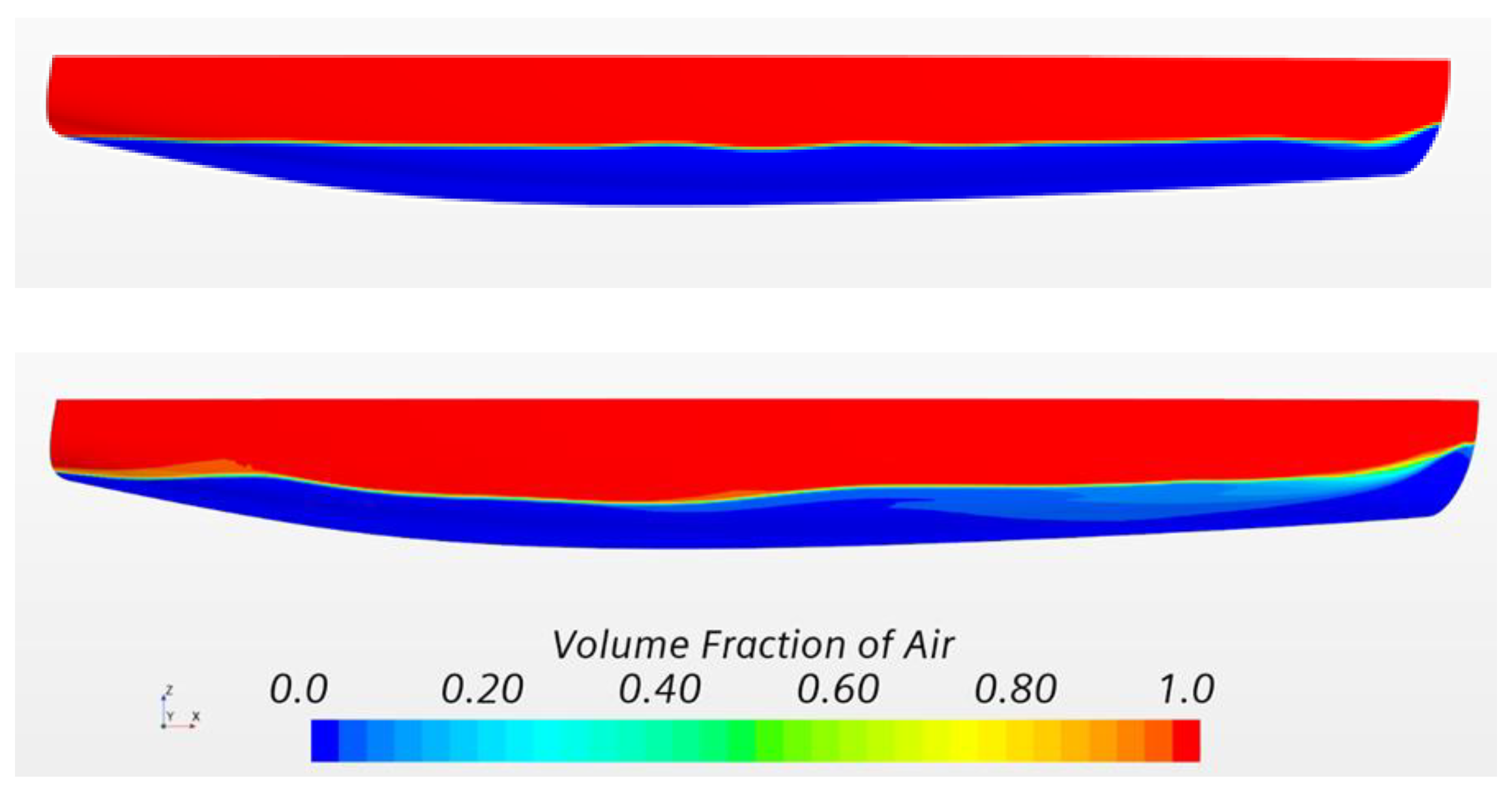
The free surface along the catamaran demihull is shown in Figure 8. It was determined based on the volume fraction of air and water. By comparing the free surfaces along the inner side of the catamaran demihull, it was evident that for $h/T=2$ at the speed of 5.5 knots, wave elevations were larger in comparison to the speed of 4 knots, resulting in significantly higher pressure resistance, Table 13.

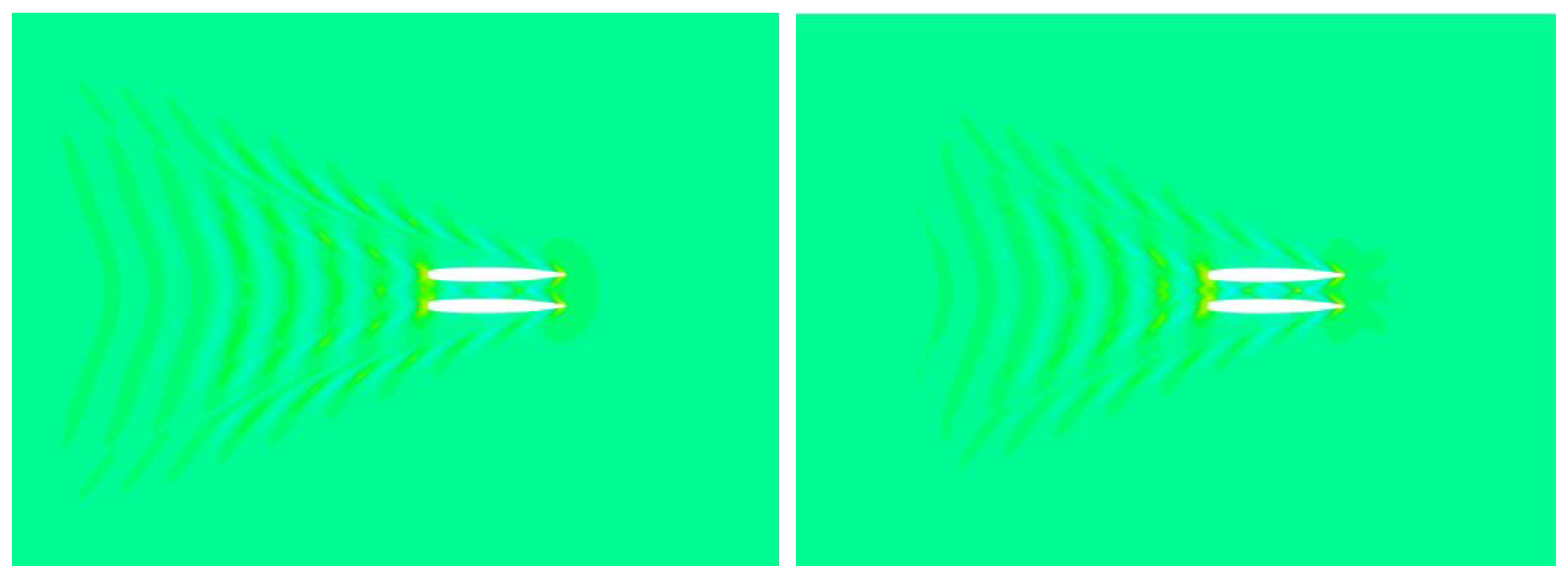
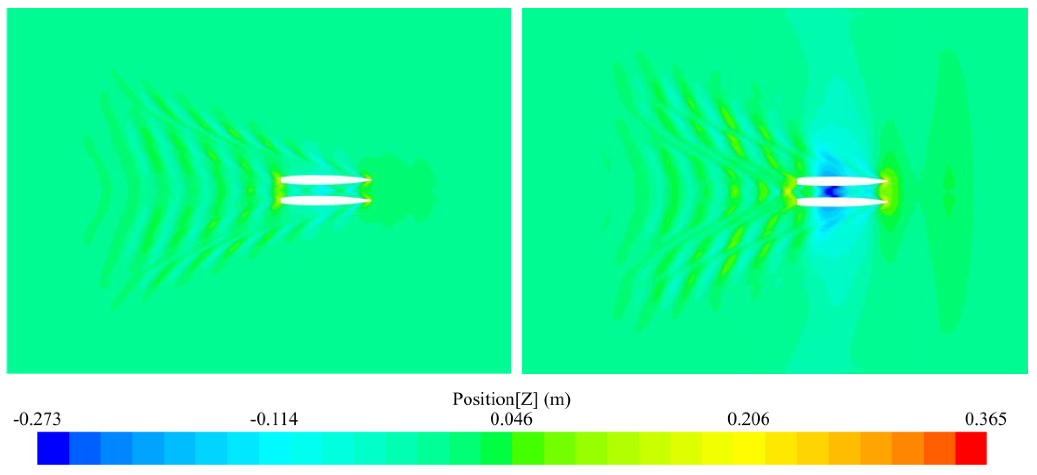
5.4. Wave Patterns

Figure 9 shows the wave patterns obtained for all the analyzed water depths at the speed of 5.5 knots. The corresponding values of the Froude number based on depth were $F{r}_h=0.4$ for $h/T=7.6$, $F{r}_h=0.55$ for $h/T=4$, and $F{r}_h=0.77$ for $h/T=2$. $F{r}_h$ for $h/T=7.6$ and $h/T=4$ fall within the range of low subcritical values, and as a result, the wave patterns resembled those in deep water. It is important to note that wave amplitudes for $h/T=4$ are somewhat higher compared to those in deep water. Additionally, a wave system consisting of transverse and diverging waves, as well as a Kelvin angle of ${19}^{\circ }{28}^{’}$, can be clearly observed. On the other hand, for $h/T=2$, a significantly larger wave trough can be observed between the catamaran demihulls in the midship area as well as larger wavelength of the transverse waves. The value of the Froude number based on depth for $h/T=2$ was $F{r}_h=0.77$ at the operational speed of 5.5 knots, which falls within the range of highly supercritical values. Accordingly, the Kelvin angle increased. Consequently, there was an increase in pressure resistance, as shown in Table 13.

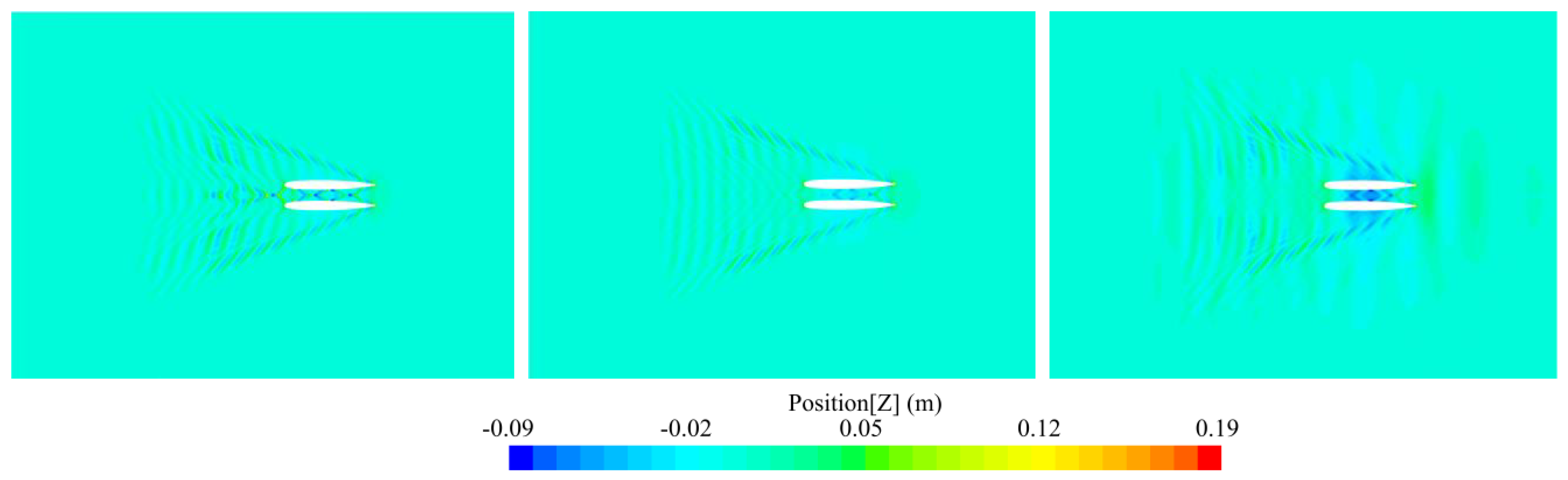
In Figure 10, the wave patterns obtained for $h/T=7.6$, $h/T=4$, and $h/T=2$ at the speed of 4 knots are shown. By reducing the speed, the value of $F{r}_h$ for $h/T=2$ was $F{r}_h=0.56$ and fell within the range of low subcritical values. The Kelvin angle was smaller compared to the one for the same depth-to-draft ratio at the speed of 5.5 knots. Larger wave elevations can be seen between the catamaran demihulls in the midship area, and the wavelength of the transverse waves is smaller in comparison to the operational speed.

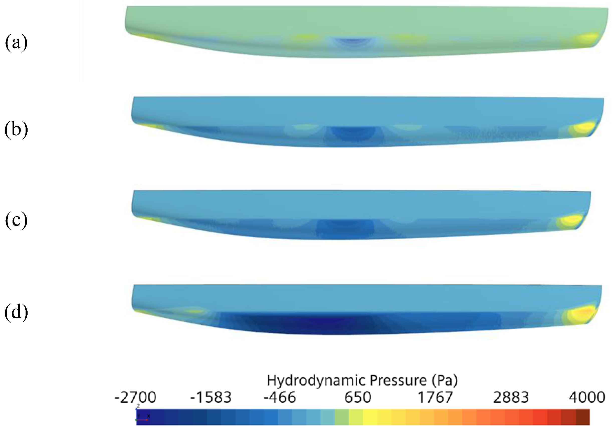
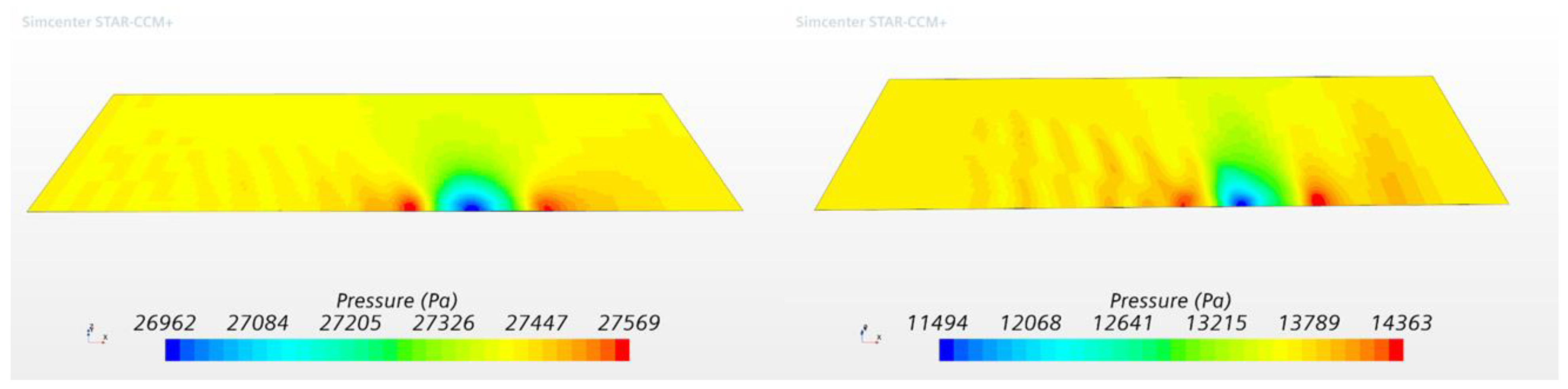
5.5. Distribution of Hydrodynamic Pressure on the Catamaran Demihull and Pressure on the Bottom

The distribution of hydrodynamic pressure along the inner side of the catamaran demihull for all the analyzed water depths at the speed of 5.5 knots is given in Figure 11. The area of high pressure at the bow is clearly visible in all cases. By comparing the obtained results, it can be seen that as the water depth decreases the overpressure in the bow area increases, while the underpressure in the midship area decreases. The decrease in the hydrodynamic pressure is a consequence of a change in the flow velocity around the catamaran hull. An increase in the flow velocity increased the tangential stresses, ultimately affecting the total resistance of the catamaran.

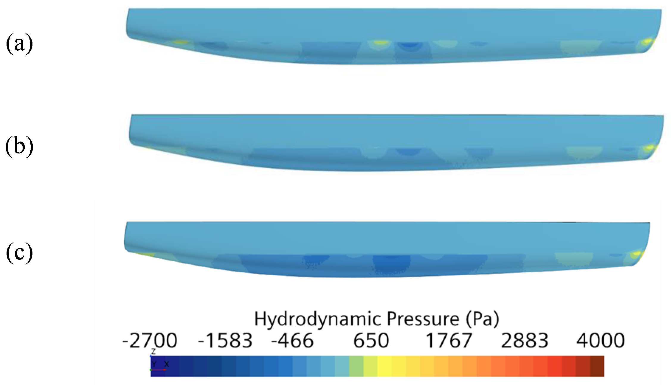
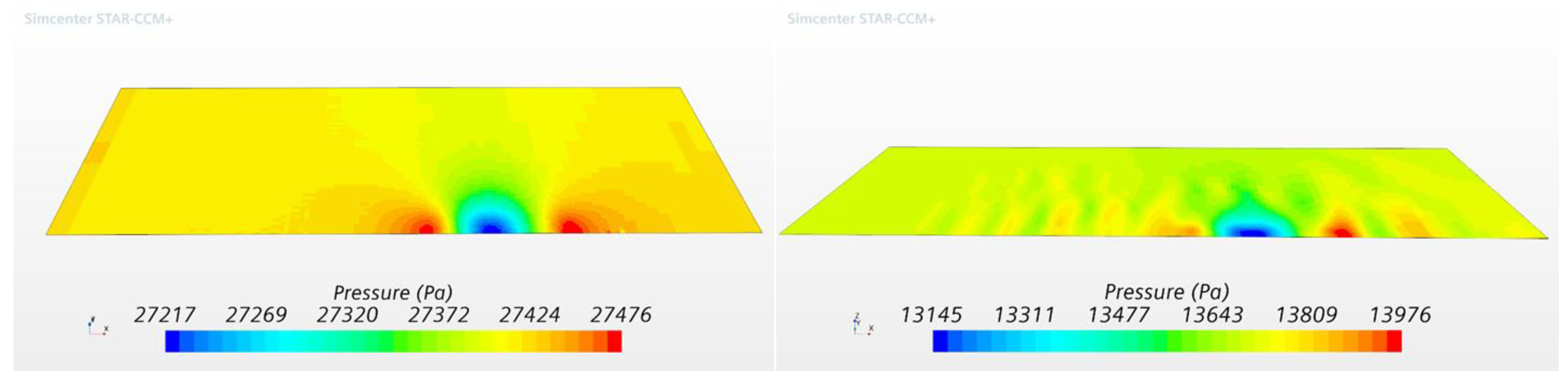
By reducing the speed by 1.5 knots, the change in the distribution of hydrodynamic pressure along the inner side of the catamaran demihull was less pronounced compared to the speed of 5.5 knots, Figure 12. Furthermore, by comparing Figure 11d and Figure 12c, a significant difference in pressure distribution can be noticed between the two analyzed speeds for $h/T=2$. Significantly lower values of hydrodynamic pressure at the operational speed can be observed, resulting in higher total resistance. Additionally, at the speed of 4 knots, lower overpressure was obtained in the bow area compared to the operational speed.

The beforementioned changes in the hydrodynamic pressure distribution correspond to changes in the pressure distribution at the bottom of the computational domain. In Figure 13, the pressure distribution on the bottom of the computational domain for $h/T=4$ and $h/T=2$ at the speed of 5.5 knots is shown, and it is evident that the pressure is significantly lower for $h/T=2$ due to the increased flow velocity between the catamaran and the bottom.

Similar results can be found by comparing the pressure distribution at the bottom of the computational domain for $h/T=4$ and $h/T=2$ at the speed of 4 knots, Figure 14.

For both $h/T=4$ and $h/T=2$, the pressure beneath the midship area was lower at the speed of 5.5 knots compared to 4 knots, while the pressure beneath the bow and stern area was slightly higher at the speed of 5.5 knots. This corresponds to the distribution of hydrodynamic pressure along the inner side of the catamaran demihull.

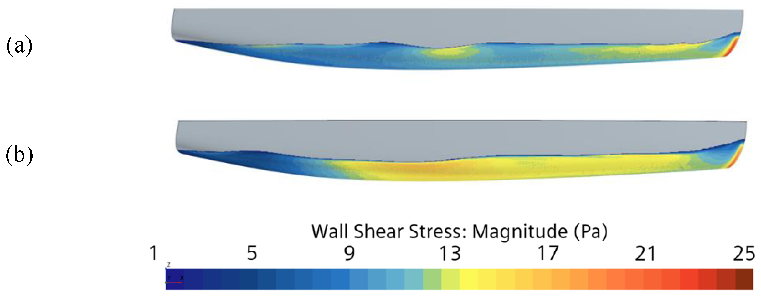
5.6. Tangential Stresses

As already mentioned, the increase in the flow velocity around the catamaran demihull leads to an increase in tangential stresses, as shown in Figure 15 for $h/T=2$ at the speed of 5.5 knots. The increase in tangential stresses is caused by the acceleration of the water flow between the catamaran and the bottom, which is particularly noticeable for $h/T=2$. The increase in tangential stresses results in an increase in frictional resistance, ultimately leading to an increase in the total resistance of the catamaran.

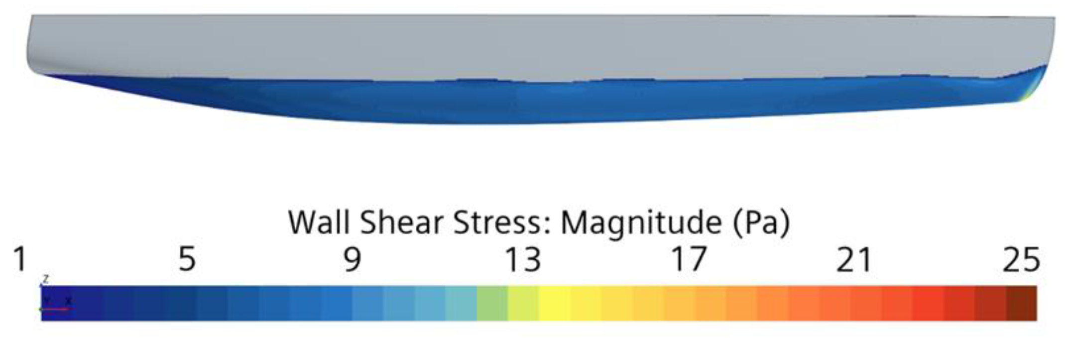
By reducing the speed to 4 knots, a significant decrease in the tangential stresses can be observed for $h/T=2$, Figure 16.

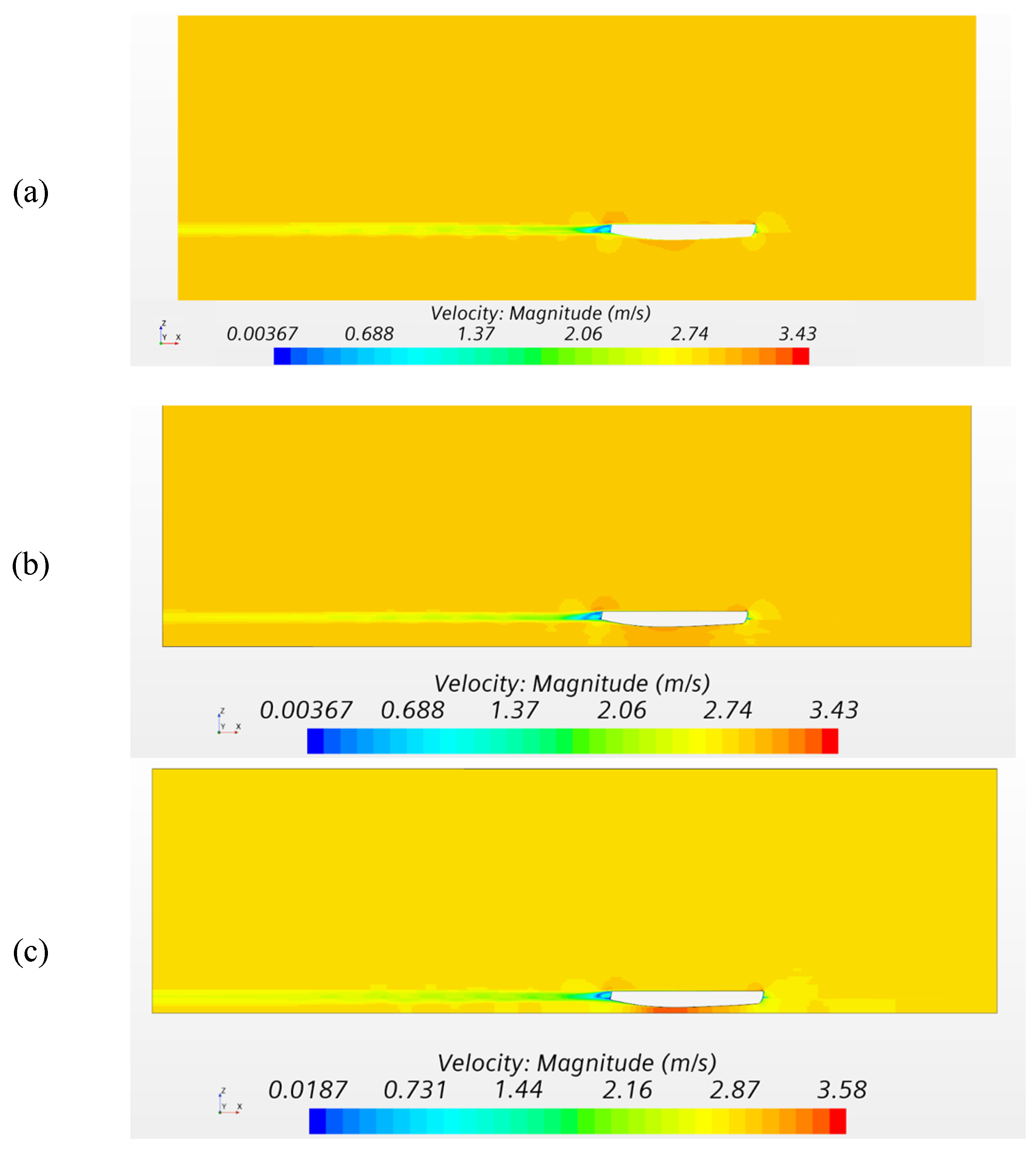
5.7. Velocity Field

The magnitude of the velocity in the symmetry plane of the catamaran demihull for all analyzed water depths at the speed of 5.5 knots is shown in Figure 17 and Figure 18. By comparing the magnitude of the velocity between the catamaran demihull and the bottom, an increase can be observed for $h/T=4$, Figure 17b in comparison to $h/T=7.6$, Figure 17a. A further reduction in depth caused a significant increase in the magnitude of the velocity at the same speed, Figure 18, which corresponded to a substantial reduction in hydrodynamic pressure and an increase in tangential stresses along the catamaran hull.

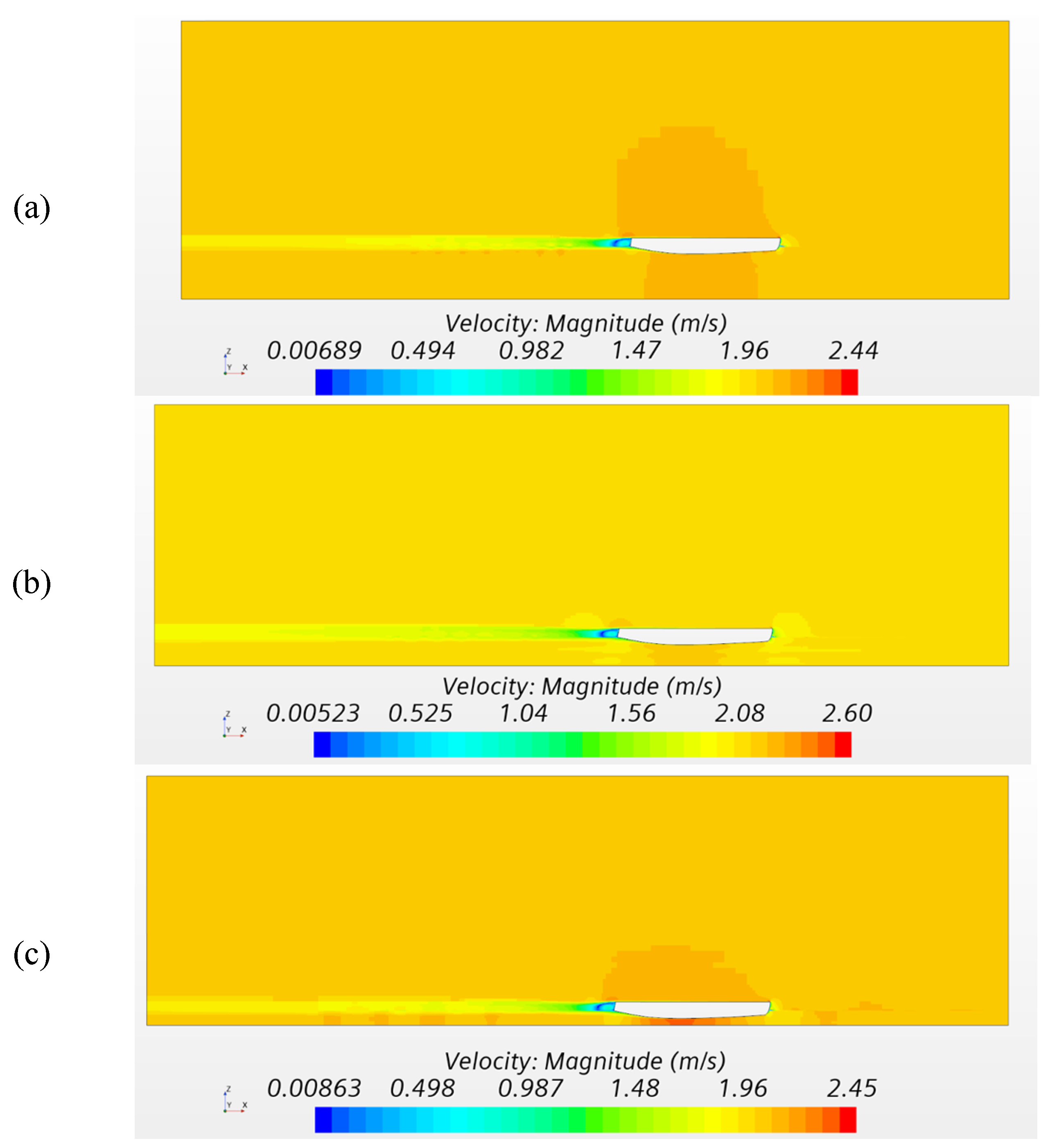
The magnitude of the velocity between the catamaran and the bottom for $h/T=7.6$ was significantly lower at the speed of 4 knots in comparison to the operational speed, Figure 18. Again, a decrease in water depth leads to an increase in the magnitude of the velocity, as can be seen in Figure 17. For $h/T=2$, it can be noticed that the maximum magnitude of the velocity between the catamaran and the bottom is approximately 30% lower when the catamaran speed is reduced from 5.5 to 4 knots.

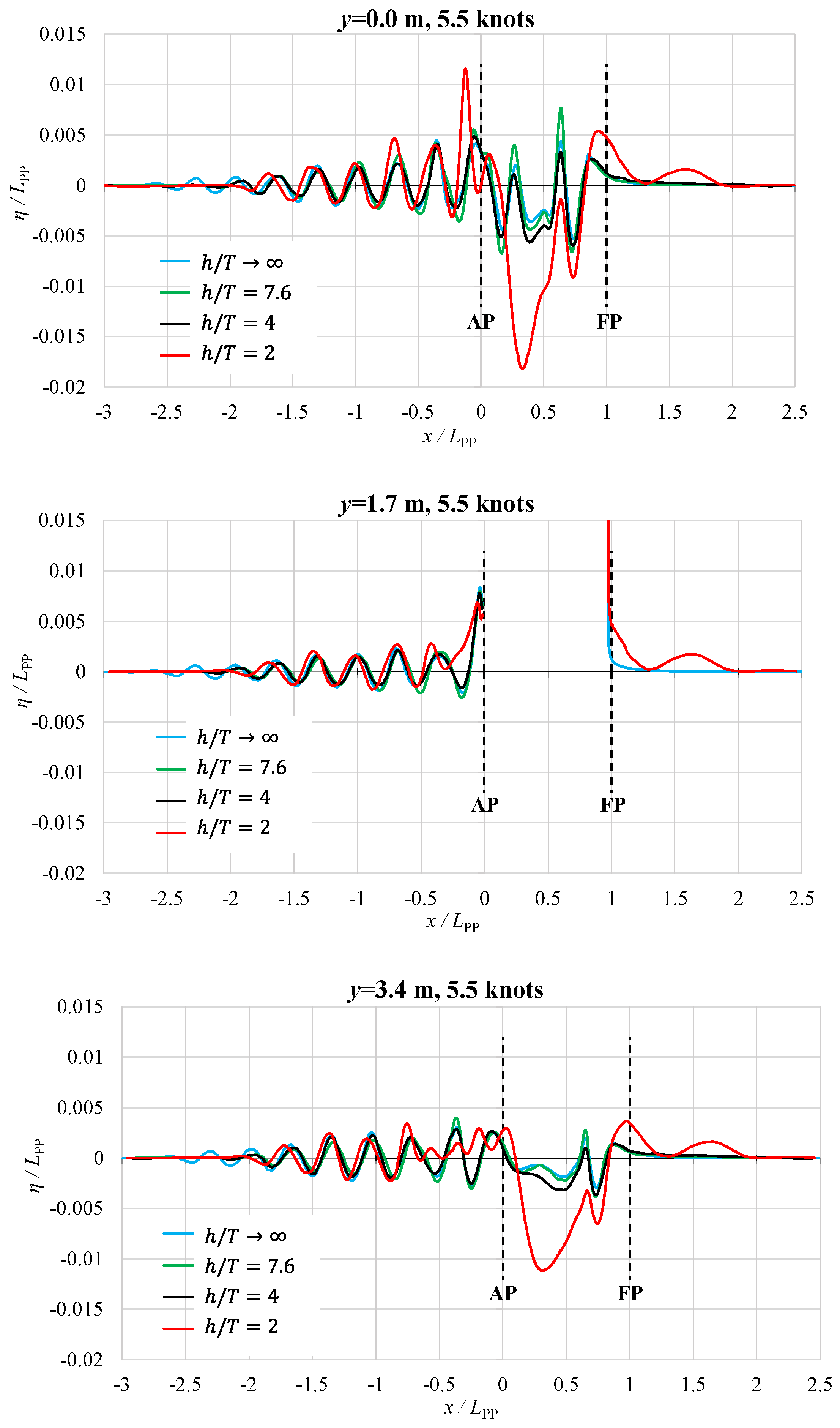
5.8. Longitudinal Wave Cuts

A comparison of the longitudinal wave cuts for all investigated water depths at the speed of 5.5. knots is given in Figure 19. The longitudinal wave cuts are given at three planes: symmetry plane, $y=1.7 \mathrm{m}$ which corresponds to the symmetry plane of the catamaran demihull, and $y=3.4 \mathrm{m}$ which corresponds to the outer side of the catamaran demihull. It can be seen that the wave elevations obtained in the catamaran symmetry plane are the largest for $h/T=2$. A significant increase in the wave elevations in front of the bow and behind the stern area, and especially in the midship area between the catamaran demihulls can be observed. It is interesting to notice that the wave elevations in the midship area between the catamaran demihulls obtained for $h/T=7.6$ are larger in comparison to the ones obtained for $h/T=4$. For $h/T=2$ the waves start to form in front of the fore perpendicular, which can be observed at all three planes.

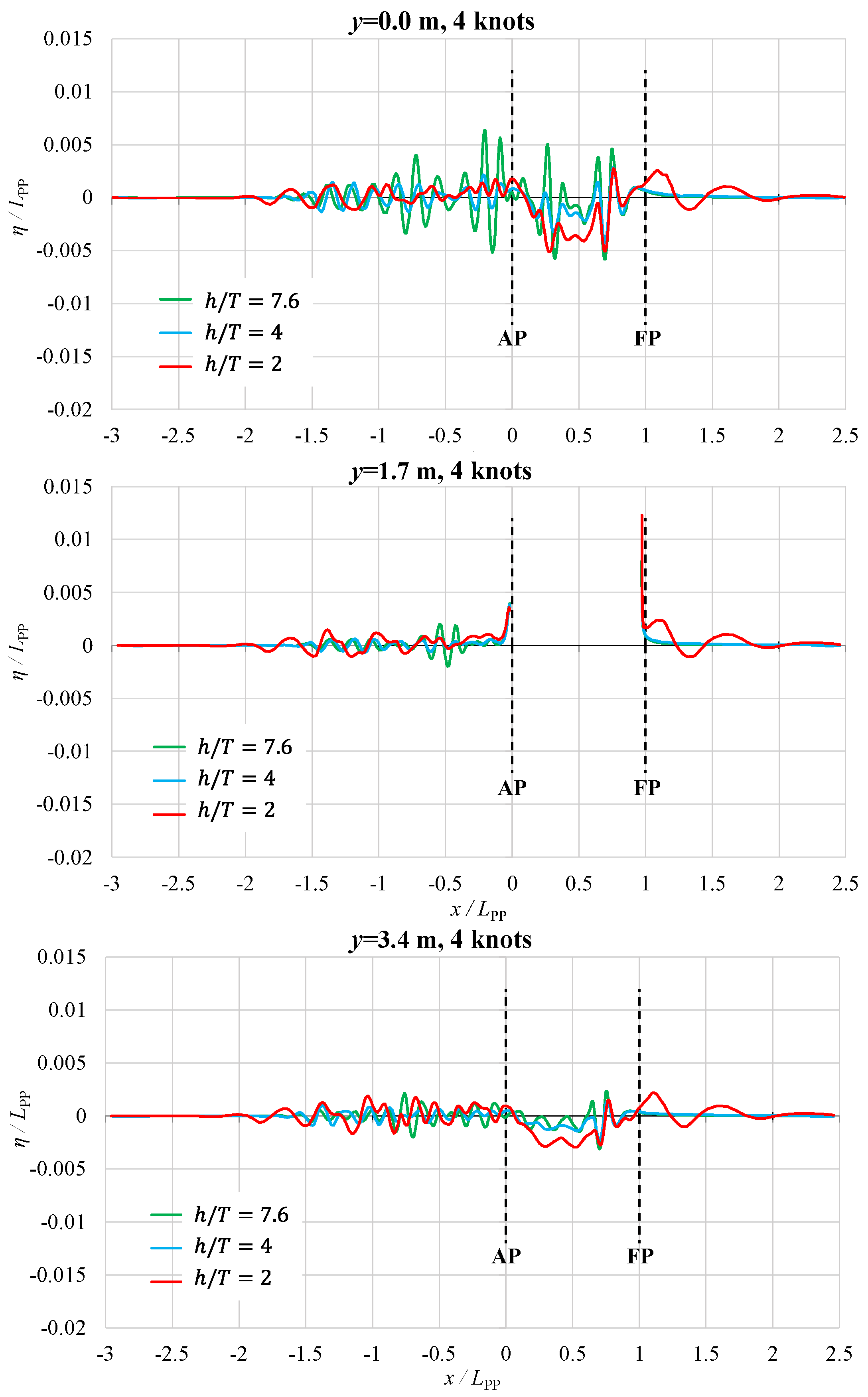
Along the outer side of the catamaran demihull, significantly larger wave troughs are formed for $h/T=2$. Again, the formation of waves in front of the fore perpendicular can be noticed. In comparison to the other analyzed water depths, the wave heights of the waves behind the stern were significantly smaller for $h/T=2$. A reduction in the wavelength for all analyzed water depths can be noticed as the speed is reduced to 4 knots, Figure 20. The largest wave elevations at the catamaran symmetry plane were observed for $h/T=7.6$. It seems that the waves generated in shallow water for $h/T=2$ have the largest wave elevations far behind the stern. The same can be observed along the symmetry plane of the catamaran demihull, as well as along the outer side of the catamaran demihull. Similar to the operating speed, the waves are formed in front of the fore perpendicular of the catamaran at the reduced speed as well.

6. Conclusions

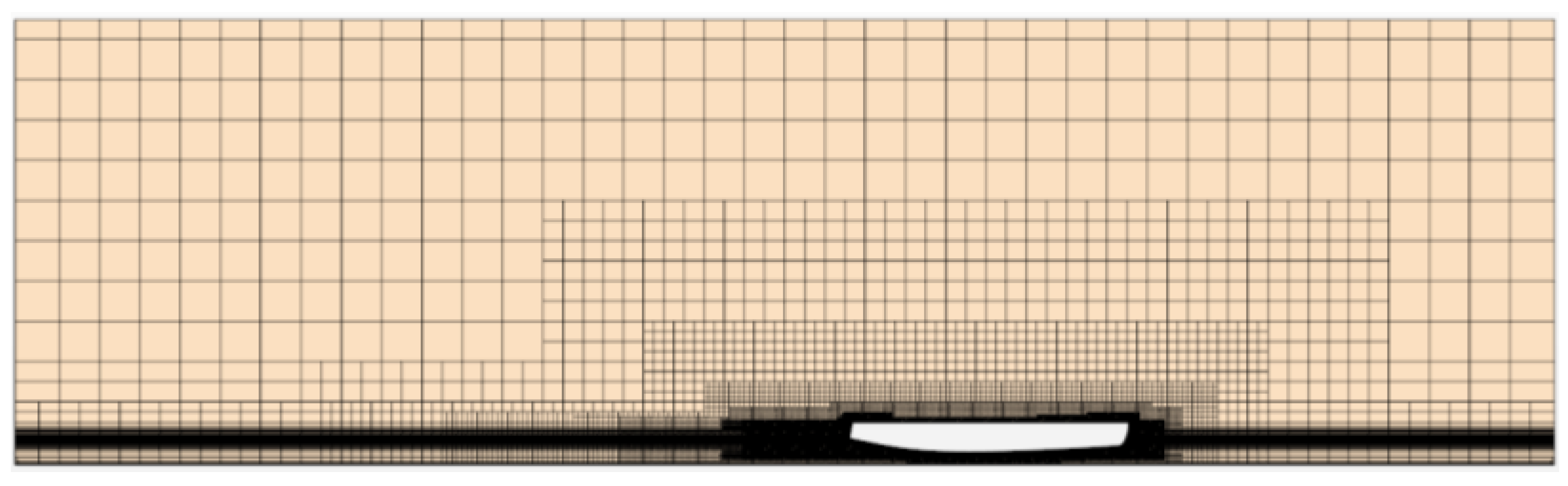
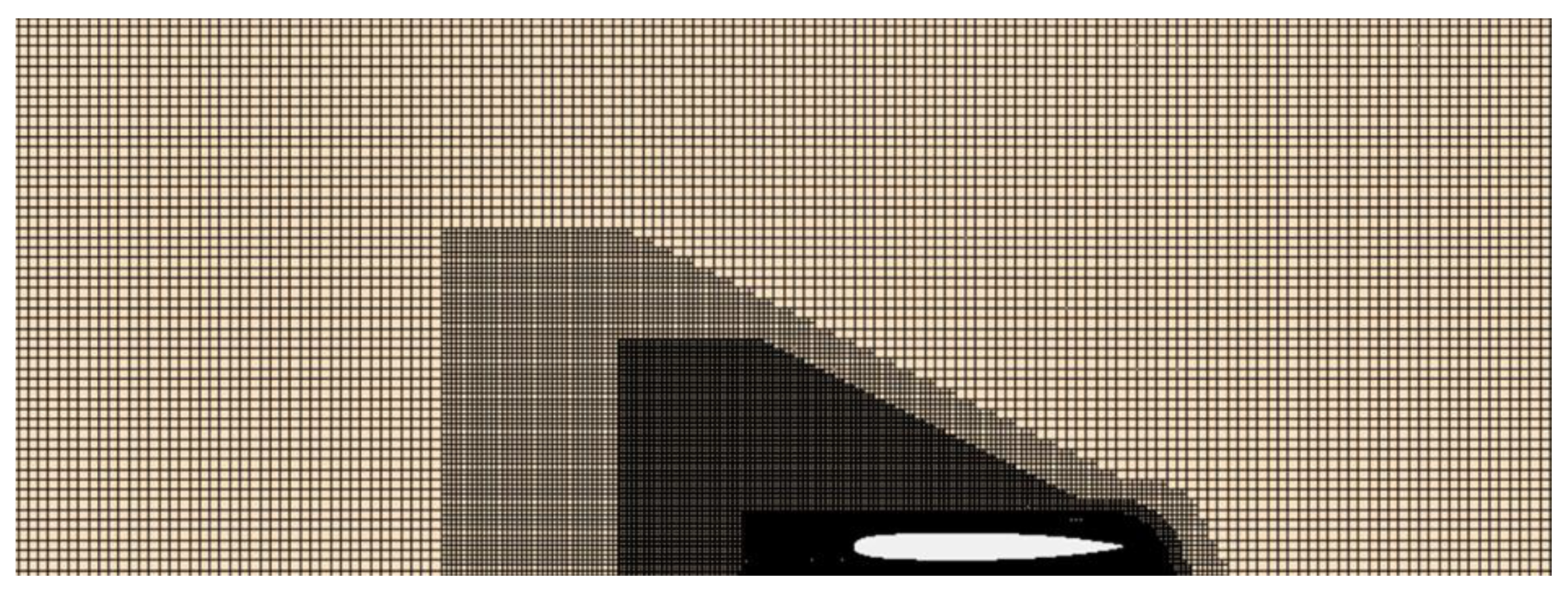
In this study, the effect of shallow water on the total resistance of a solar catamaran was numerically assessed in deep water and for three different depths at two speeds. The numerical simulations were performed using the commercial software package STAR-CCM+. A mathematical model based on the Reynolds-averaged Navier–Stokes (RANS) equations along with the $k-\omega$ SST turbulence model was used. The computational domain and the governing equations were discretized using the finite volume method, and the volume of fluid method was employed to determine the position of the free surface. Within the numerical simulations in shallow water, a mesh morphing algorithm was used to accommodate possibly more pronounced catamaran motions. Based on the performed verification study, the numerical uncertainty of total resistance and sinkage of the catamaran in deep water and for $h/T=2$ was calculated at the speed of 5.5 knots. The obtained numerical uncertainty of the total resistance of the catamaran in shallow water is somewhat higher in comparison to the deep water, which is in line with expectations considering that the mesh requirements are higher.

The speed reduction for $h/T=2$ was determined based on Schlichting’s diagram which proved to be very practical for estimating the speed reduction in shallow water, intending to avoid negative effects such as potential grounding or stranding. By analyzing the obtained numerical results, it can be concluded that the total resistance of the catamaran at the operational speed of 5.5 knots increased significantly as the depth decreased, resulting in notable sinkage of the catamaran. On the other hand, it was noticed that the shallow water did not have a significant effect on catamaran trim in this particular case. A reduction in speed by 1.5 knots led to a significant decrease in the total resistance as well as sinkage of the catamaran.

The effect of shallow water on the total resistance of the catamaran was also manifested through the wave pattern. In the case of $h/T=2$ at the operational speed of 5.5 knots, the Kelvin angle increased along with the wavelength of the transverse waves, increasing the pressure resistance. The decrease in the hydrodynamic pressure along the catamaran demihull is a consequence of a change in the flow velocity. An increase in the flow velocity increased the tangential stresses, ultimately affecting the total resistance of the catamaran. The changes in the distribution of hydrodynamic pressure correspond to changes in the pressure distribution at the bottom of the computational domain. By analyzing the magnitude of the velocity at the symmetry plane of the catamaran demihull, it was noticed that the maximum magnitude of the velocity between the catamaran and the bottom was approximately 30% lower when the catamaran speed was reduced from 5.5 to 4 knots. By analyzing the longitudinal wave cuts, a significant increase in the wave elevations in front of the bow and behind the stern, and especially in the midship area between the catamaran demihulls was observed for the smallest water depth.

It has been demonstrated that the application of computational fluid dynamics enables a detailed analysis of the flow around the catamaran in shallow water conditions, allowing for the determination of the increase in total resistance and changes in sinkage and trim, to avoid potential negative effects associated with sailing in confined waterways.