Article

Adaptive Beamforming with Hydrophone Arrays Based on Oblique Projection in the Presence of the Steering Vector Mismatch

1
School of Marine Science and Technology, Northwestern Polytechnical University, Xi’an 710072, China
2
Shaanxi Key Laboratory of Underwater Information Technology, Xi’an 710072, China
*
Author to whom correspondence should be addressed.
J. Mar. Sci. Eng. 2023, 11(4), 876; https://doi.org/10.3390/jmse11040876
Submission received: 27 March 2023 / Revised: 13 April 2023 / Accepted: 18 April 2023 / Published: 20 April 2023
(This article belongs to the Special Issue Underwater Acoustics and Digital Signal Processing)

Abstract

:
In sonar systems, the performance of adaptive beamformers severely degrades when mismatches occur between the actual and presumed steering vectors of the desired signal, mainly due to hydrophone position errors, amplitude-phase errors, and the scattered effect of arrays. Similarly, an inadequate number of “training” samples can lead to performance degradations similar to those caused by mismatches. In this paper, an adaptive beamforming algorithm based on oblique projection (OP-ABF) mismatch compensation is proposed to remove the degradation caused by the arbitrary-type steering vector mismatch of the desired signal. The proposed algorithm is motivated by the fact that the weight vector of adaptive beamforming can be represented as a linear combination of the optimal one and the oblique projection (OP) vector, which is generated by the steering vector mismatch and does not exist without this. Our algorithm was developed by constructing the oblique projection mismatch compensation vector (OPMCV) to provide the minimum variance distortionless response (MVDR) beamformer. Then, the algorithm could be implemented by the solution of the OP matrix with the formulation of the covariance matrix loading (CML). The simulation results of a uniform linear array (ULA) and a half-cylindrical conformal array (HCCA) show that the OP-ABF can optimize the original weight vector as much as possible without sacrificing the output signal-to-interference-plus-noise ratio (SINR) under different conditions. Experimental results for the HCCA also confirm the effectiveness of this algorithm.

1. Introduction

Array signal processing is widely used in modern sonar systems, and adaptive beamforming is one of the important techniques [1,2,3]. It has obvious advantages over other methods in improving the detection performance of sonar in complex ocean environments [4,5]. Among many adaptive beamfomers, the minimum variance distortionless response (MVDR) beamformer [6] can theoretically maximize the output signal-to-interference-plus-noise ratio (SINR), provided that there is no desired signal in the received data or the characteristics of the desired signal are precisely known.
As we know, however, the performance of adaptive beamformers is sensitive to array and model imperfections. The desired signal is always present in the received data in many scenarios, such as passive sonar detection and underwater communication. Further, there are many reasons causing the steering vector (SV) mismatch of the desired signal, such as the sensor position errors [7], the amplitude-phase errors [8], and the scattered effect generated by the rigid baffle where hydrophones are mounted [9]. Interestingly, the influence of the snapshot deficiency [10] can be also somehow mathematically considered as the SV mismatch. The SV mismatch degrades the performance of the MVDR beamformer, especially when the received data contain the desired signal component [11,12], even though the mismatch is slight between the actual and presumed steering vectors of the desired signal. In sonar systems, therefore, the SV mismatch poses a serious challenge to the adaptive beamforming performance. Several approaches are known to provide an improved performance against the SV mismatch. The diagonal loading (DL) technique [13] is one of the most widely used methods to solve this problem. Although only one parameter is required to be calculated in the DL beamformers [14,15], they sacrifice the output SINR, and do not remove the SV mismatch in essence.
To overcome shortcomings of the DL beamformers, the interference-plus-noise covariance matrix (INCM) reconstruction is proposed [16]. The INCM can reduce the influence of the SV mismatch of the desired signal on the adaptive beamforming performance, and further improve the output SINR of adaptive beamformers compared with the DL beamformers. At present, a variety of INCM algorithms have been developed, which mainly include sparse reconstruction methods [17,18] based on the spatial sparsity of signals, subspace methods [19,20] according to characteristics of the eigen-subspace of the sample covariance matrix, and convex optimization methods [21,22]. A high computational cost is required in the INCM for high-resolution spatial spectrum estimation, which is sensitive to environmental parameters and cannot be implemented well in the ocean. Since the desired signal and interferences lie in the same eigen-subspace, the INCM leads to the coherence of the desired signal and interferences, which degrades the performance of adaptive beamformers. Therefore, it is crucial to the performance of the INCM algorithms whether the desired signal and interferences can be perfectly separated from the eigen-subspace of the covariance matrix of the received data. These drawbacks make them difficult to promote in underwater acoustic signal processing.
In addition to the shortcomings mentioned above, in sonar, a major reason for the poor performance of the adaptive beamformers is the fact that the mismatch, the desired signal, and interferences are not orthogonal in the signal subspace. This means that eliminating the mismatch comes at the cost of reducing the interference suppression, while maintaining the interference suppression can retain a part of the mismatch component in the received signal, which is also the reason why adaptive beamformers based on orthogonal projection or eigen-decomposition [23,24,25,26] are restricted. It is difficult to remove the SV mismatch thoroughly in such cases. Therefore, in underwater signal processing, developing an algorithm of adaptive beamforming that can cope with the SV mismatch caused by arbitrary-type errors and is convenient for implementation on hydrophone arrays on the premise of the high performance of the adaptive beamforming is a challenging issue.
As a general representation of the orthogonal projection, the oblique projection (OP) only requires subspaces that are mutually disjoint from each other. That is, bases spanning different subspaces are not orthogonal but uncorrelated [27]. This characteristic makes it possible to only eliminate the SV mismatch of the desired signal in the signal subspace. The OP operator is first used to remove the intersymbol interference [28] in communications, and then is widely used in mainlobe interference suppression [29,30]. In recent years, algorithms of array response control based on the OP have been developed [31,32,33]. Based on the above discussion, the OP can play an important role and provide us with a way to improve the performance of adaptive beamforming.
In this paper, we apply the OP to sonar signal processing and propose an adaptive beamforming algorithm based on oblique projection (OP-ABF), aiming at eliminating the SV mismatch in the received data to improve the output SINR. More specifically, the mismatch term in the initial weight vector can be expressed as the OP vector in a determined but unknown subspace. In order to eliminate the mismatch term, the original problem is converted to the covariance matrix loading (CML) problem, which can be regarded as a generalization of the conventional DL [34]. The OP matrix and undetermined parameters are solved by taking advantage of eigen-decomposition of the covariance matrix of the received data. The optimized weight vector is finally derived, in which the mismatch term has been compensated by the vector called the OP mismatch compensation vector (OPMCV). The advantages of the proposed OP-ABF algorithm are not only that it can perfectly remove the arbitrary-type SV mismatch, but also that it is implemented by only using the received data without any other prior information such as the upper bound of the error norm or the high resolution spatial spectrum. Another valuable point is that the proposed OP-ABF has no restriction on the array geometry, which is practically applicable to arrays of different underwater platforms.
The rest of the paper is organized as follows. In Section 2, the signal model, and some necessary concepts regarding the adaptive beamforming are introduced, respectively. The proposed OP-ABF is presented and we provide an approach that can resolve the undetermined parameters in Section 3. The interpretation and necessary analysis of the proposed OP-ABF are given in Section 4. Representative results are presented in Section 5 and conclusions are drawn in Section 6.

2. Problem Formulation

Let us denote matrices and vectors as bold upper-case and lower-case letters, respectively. In particular, I is used to stand for the identity matrix. R and C denote the sets of real and complex numbers, respectively. R · and N · are the column space and the null space of the input matrix, respectively. R · is the orthogonal complementary space of R · . P · is the eigenvector corresponding to the maximum eigenvalue of the input matrix.

2.1. Signal Model

Consider an array with an arbitrary configuration composed of identical M omni-directional hydrophones. Suppose there are D far-field narrowband uncorrelated signals impinging on the array, one of which is the desired signal while the other D 1 are interferences. The signals received by the array can be written [12] as
y ( t ) = a asv s 0 t + d = 1 D 1 a d s d ( t ) + n ( t )
where
  • t: arbitrary sampling time.
  • y ( t ) C M × 1 : the received data sampled by the array.
  • a asv : the actual SV of the desired signal.
  • a d : the SV of the dth interference.
  • s 0 t : the wavefront of the desired signal.
  • s d ( t ) : the wavefront of the dth interference.
  • n ( t ) : the zero mean Gaussian white noise, representing additive noise in the environment received by the array.
Assuming that the desired signal, interferences, and noise are uncorrelated with each other, noise on each hydrophone is also uncorrelated. The covariance matrix of y ( t ) is given as
R y = E y ( t ) y H ( t ) = R s + R int + n = σ s 2 a asv a asv H + d = 1 D 1 σ d 2 a d a d H + σ n 2 I
where
  • E · : the statistical expectation.
  • R s = σ s 2 a asv a asv H : the covariance matrix of the desired signal.
  • R int + n = d = 1 D 1 σ d 2 a d a d H + σ n 2 I : the covariance matrix of interference-plus-noise.
  • σ n 2 I : the covariance matrix of the Gaussian white noise.
  • σ s 2 : the power of the desired signal.
  • σ d 2 : the power of the dth interference.
  • σ n 2 : the power of noise.
In practice, the covariance matrix of y ( t ) is estimated by a finite number of samples. The sample covariance matrix of y ( t ) is written as
R ^ = 1 L t = 1 L y t y H t
where
  • L: the sample size.
  • · H : the conjugate-transpose operator.
The output of the beamformer is the weighted summation of the received data [35], i.e.,
p = w H y t
where w denotes the weight vector of the beamformer. Then, the power of the beamformer output is given [12,35] as
σ p 2 = E p p * = w H R y w = w H R s w + w H R int + n w
where the superscript · * is the conjugate operator.
According to the signal model given in (1) and the covariance matrix given in (2), the input signal-to-noise ratio (SNR) of the beamformer is defined as
SNR in = σ s 2 / σ n 2
Therefore, the output signal-to-interference-plus-noise ratio (SINR) of the beamformer is given as
SINR out = w H R s w w H R int + n w = σ s 2 σ n 2 · w H a 0 2 w H ρ int + n w
where
  • ρ int + n : the normalized interference-plus-noise covariance matrix of R int + n with respect to the power of noise.
  • a 0 : the presumed SV of the desired signal.
Ideally, the presumed SV and the actual one can point in the same direction as the desired signal, i.e., a asv = a 0 , and the normalized SINR out of the beamformer regarding SNR in is written from (6) and (7) as
G = SINR out SNR in = w H a 0 2 w H ρ int + n w
where G is defined as spatial processing gain (SPG) in this paper because there are interferences in signal model (1). The SPG is the normalized SINR out with respect to σ n 2 for the presence of interferences [35].
In practice, the actual SV of the desired signal is unknown and inevitably deviates from the presumed one, i.e., a asv a 0 . We make the following assumptions regarding the presumed SV a 0 and the actual one a asv of the desired signal.
1: a asv is different from a 0 , i.e., a asv = a 0 + δ , where δ denotes the SV mismatch caused by arbitrary-type errors mentioned in the Introduction.
2: a 0 represents the presumed SV of the desired signal, but it cannot be used directly since it is polluted by δ in the received data.
3: a asv is the actual SV of the desired signal, in the direction of which we hope the SINR out of adaptive beamformers will be maximized although it contains the mismatch vector δ .
We can now state the problem as follows: given the received data y ( t ) , eliminate the SV mismatch of the desired signal and achieve the maximum SINR out .

2.2. Adaptive Beamforming

The optimal beamformer in adaptive beamformers in terms of maximizing the SINR out is derived from the MVDR beamformer [6], and its weight vector and SINR out are expressed, respectively, as
w MVDR = α ρ int + n 1 a 0
SINR out , MVDR = σ s 2 σ n 2 · w MVDR H a 0 2 w MVDR H ρ int + n w MVDR = σ s 2 / σ n 2 · a 0 H ρ int + n 1 a 0
where α = a 0 H ρ int + n 1 a 0 1 is a normalization factor that guarantees the distortionless response constraint in the direction of a 0 and does not affect its SINR out .
In sonar, ρ int + n in (9) cannot be obtained and is replaced by the sample covariance matrix given in (3). Thus the generalized version of adaptive beamformers known as the sample matrix inversion (SMI) beamformer is derived, and its weight vector and SINR out are expressed, respectively, as
w SMI = β R ^ 1 a 0
and
SINR out , SMI = σ s 2 σ n 2 · w SMI H a 0 2 w SMI H ρ int + n w SMI = σ s 2 / σ n 2 · a 0 H R ^ 1 a asv 2 a 0 H R ^ 1 ρ int + n R ^ 1 a 0
where β = a 0 H R ^ 1 a 0 1 plays the same role as α . Equations (11) and (9) are equivalent on the premise that the desired signal component in R ^ is exactly known.
In passive sonar systems, the desired signal component is always present in the received data. Once the SV mismatch is introduced into the estimation of R ^ , the performance of the SMI beamformer dramatically degrades no matter how slight the mismatch is. In order to solve this problem, a popular kind of algorithms are the diagonal loading (DL) methods, which are referred here as the loading sample matrix inversion (LSMI) beamformer [12] and given here:
w LSMI = η R ^ + γ I 1 a 0
where η is a normalization factor and γ is defined as γ = σ n 2 · 10 LNR / 10 , where LNR is called the load-to-white-noise ratio.
The LSMI beamformer alleviates the performance degradation caused by the SV mismatch to some extent. However, the LSMI beamformer cannot completely eliminate the SV mismatch of the desired signal in the received data. In recent years, adaptive beamformers based on the interference-plus-noise covariance matrix (INCM) reconstruction provide an improved performance against the SV mismatch [18,20,21,22]. The INCM provides “the desired signal-free” “training” data as accurately as possible at the expense of sufficient prior information and computational complexity.

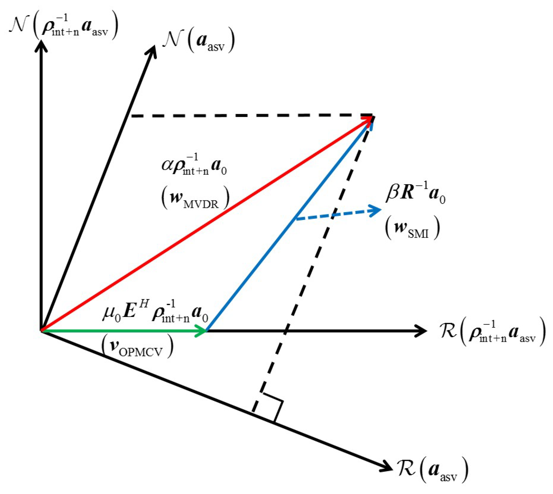
3. The Proposed Algorithm Based on OP

3.1. The OP-ABF Algorithm

Using the matrix inversion lemma [27], R ^ 1 in (11) can be written as
R ^ 1 = σ n 2 I ρ int + n 1 a asv a asv H σ s 2 / σ n 2 1 + σ s 2 / σ n 2 a asv H ρ int + n 1 a asv ρ int + n 1 = σ n 2 I σ s 2 / σ n 2 a asv H ρ int + n 1 a asv 1 + σ s 2 / σ n 2 a asv H ρ int + n 1 a asv · ρ int + n 1 a asv a asv H a asv H ρ int + n 1 a asv ρ int + n 1 = σ n 2 I μ 0 · E H ρ int + n 1
where
μ 0 = σ s 2 / σ n 2 a asv H ρ int + n 1 a asv 1 + σ s 2 / σ n 2 a asv H ρ int + n 1 a asv
is a real number whose magnitude is proportional to the SNR in and is in the range 0 μ 0 < 1 .
E H = ρ int + n 1 a asv a asv H a asv H ρ int + n 1 a asv
is an idempotent and non-Hermitian matrix, i.e., E H = E H 2 and E H E . A matrix that satisfies these mathematical properties is called an oblique projection (OP) matrix. For E H in (16), it is the OP matrix projecting onto R ρ int + n 1 a asv along the direction parallel to R a asv , so R E H is equal to R ρ int + n 1 a asv , and N E H contains R a asv . A detailed interpretation of the OP is given by [27], which can be found in the Appendix A.
Substituting (14) into (11) and w SMI results in:
w SMI = β / σ n 2 · I μ 0 · E H ρ int + n 1 a 0 = β / σ n 2 · ρ int + n 1 a 0 β / σ n 2 · μ 0 E H ρ int + n 1 a 0
where β / σ n 2 does not affect the performance and can be omitted below. It is shown in (17) that the SMI beamformer is a linear combination of two vectors. One is the MVDR beamformer, which provides the highest possible SINR out . The other is the projection of this MVDR beamformer in R E H , which is generated by the SV mismatch. When a asv = a 0 , R ρ int + n 1 a asv = R ρ int + n 1 a 0 , and E H ρ int + n 1 a 0 = ρ int + n 1 a 0 , the SMI beamformer is reduced to the standard MVDR beamformer. The projection of the MVDR beamformer in R E H does not lie in the same linear space as itself in the presence of the SV mismatch in adaptive beamforming, which leads to the deviation of the SMI beamformer from the optimal one and the performance of itself degrading.
We define the oblique projection mismatch compensation vector (OPMCV) as
v OPMCV = μ 0 E ^ H ρ ^ int + n 1 a 0
where E ^ H and ρ ^ int + n 1 denote the estimates of the corresponding matrices, respectively.
Correspondingly, the geometric explanation of w MVDR , w SMI and v OPMCV is illustrated in Figure 1. Three vectors form a triangle in the presence of the SV mismatch. w MVDR does not lie in R ρ int + n 1 a asv when a asv a 0 . According to (17), w SMI (blue arrow) is otherwise the difference between w MVDR (red arrow) and v OPMCV (green arrow). Since μ 0 is proportional to the SNR in , the greater the SNR in , the larger the angle between w SMI and w MVDR , indicating that the SINR out , SMI severely decreases.
The core idea of the adaptive beamforming based on oblique projection (OP-ABF) is to estimate the oblique projection matrix E ^ H by the received data. Once the OPMCV is obtained, the MVDR beamformer is derived by an arithmetical manipulation from (9) and (17):
w MVDR = α w SMI + v OPMCV
Ignoring the normalization factor α and substituting E ^ H and w SMI in (11) into (19), the expression in brackets at the right hand of the equation is rewritten as
w SMI + v OPMCV = σ n 2 R ^ 1 + σ n 2 μ 0 E ^ H ρ ^ int + n 1 a 0
Applying the Woodbury matrix identity [27] to the expression in brackets at the right hand of the equation in (20), we can derive
R ^ 1 + σ n 2 μ 0 E ^ H ρ ^ int + n 1 1 = I + σ n 2 μ 0 R ^ E ^ H ρ ^ int + n 1 1 R ^ = R ^ μ α v 1 H R ^ v 1 1 + μ α E R ^
where
  • μ α : an undetermined real number.
  • v 1 = P E ^ : the principal component of E ^ .
  • E R ^ = v 1 ( v 1 H R ^ v 1 ) 1 v 1 H R ^ : an oblique projection matrix.
The derivation of (21) uses two properties of E ^ H : its eigenvalues are only 0 or 1, and Rank ( E ^ H ) = Rank [ R ( ρ ^ int + n 1 a ^ a s v ) ] = 1 . Substituting (20) and (21) into (19), this is rewritten as
w MVDR = α σ n 2 R ^ μ α v 1 H R ^ v 1 1 + μ α E R ^ 1 a 0 = α R ^ μ α v 1 H R ^ v 1 1 + μ α E R ^ 1 a 0
where α is also a normalization factor.
By comparing (22) with (13), it can be found that each entry in R ^ is “loaded” in (22) by the OP matrix while only diagonal entries in R ^ are loaded in (13) by the identity matrix. This means that the OP operation on the R ^ can be seen as a special case of the covariance matrix loading (CML) method, where the loading matrix is the rank-1 OP matrix E R ^ . The covariance matrix R ^ after the CML no longer contains the desired signal component, and the mismatch is eliminated without affecting the rest of R ^ , which indicates that the interference suppression is not reduced. w MVDR in (22) continues to be formulated as
w MVDR = α R ^ 1 I + μ α E ^ a 0
As a result, μ α and E ^ are parameters that need to be solved for w MVDR . The OP-ABF is eventually written as
w OP = α R ^ 1 I + μ α E ^ a asv
As we will see in the next subsection, a asv is to be derived in the solution of E ^ .

3.2. Solutions of E and μα

The covariance matrix of the received data R ^ can be eigen-decomposed as
R ^ = U Λ U H = i = 1 M λ i u i u i H
where
  • Λ = diag λ 1 , λ 2 , , λ m , , λ M : the eigenvalue matrix in which eigenvalues are in descending order.
  • U = u 1 , u 2 , , u M = [ U s , U n ] : the eigenvector matrix corresponding to the eigenvalues.
  • U s : the eigenvectors that span the signal-plus-interference subspace associated with dominant eigenvalues.
  • U n : the eigenvectors that span the noise subspace.
The desired signal SV and the interference SVs lie in U s , which are formulated as
a asv a a = U s e s 0 , e s 0 , e s 0 R D × 1 a d i a a = U s e d i , e d i , e d i R D × 1 , i = 1 , D 1
where
  • e s 0 : the linear coefficient vector of a asv .
  • e d i : the linear coefficient vector of a d i .
  • a : a random vector that lies in U s or U n .
Assume that the desired signal is located at a certain angle sector, and we can define R ^ s as the virtual covariance matrix of the desired signal. R ^ s is roughly estimated by the MVDR spatial spectrum over an angular sector as
R ^ s = Φ a i ϕ a i H ϕ a i H ϕ R 1 a i ϕ d Φ
where
  • Φ = ϕ 0 Δ , ϕ 0 + Δ : the angle sector centering at the direction of a 0 with a range of 2 Δ .
  • ϕ 0 : the bearing of a 0 .
For the convenience of computation, replacing the integral in (27) by summation, R ^ s in (27) can be approximately expressed as
R ^ s = p = 1 P a i ϕ p a i H ϕ p a i H ϕ p R 1 a i ϕ p
where
  • a i ϕ p : the nominal SV at ϕ p that is uniformly sampled in Φ .
  • P: the number of samples in Φ .
Let E ^ s denote the eigenvector matrix corresponding to the dominant eigenvalues, which are derived from the eigen-decomposition of R ^ s . Similarly, the desired signal SV lies in E ^ s , which is reformulated as
a asv a a = E ^ s e s 1 , e s 1 R L s × 1
where
  • e s 1 : a linear coefficient vector in the set in (29).
  • L s : the dimension of E ^ s .
From (26) and (29), a asv lies in the intersection of U s and E ^ s . Therefore, a asv can be estimated by
a ^ asv = M P P U s P E ^ s
where
  • P U s = U s U s H : the orthogonal projection matrix of U s
  • P E s = E ^ s E ^ s H : the orthogonal projection matrix of E ^ s .
Similarly, a d i can be also estimated by the following equation
[ a ^ d 1 , , a ^ d D 1 ] T = M P P U s P E ^ int
where P E ^ int = E ^ int E ^ int H represents the orthogonal projection matrix of E ^ int , which contains the dominant eigenvectors obtained by eigen-decomposition of the matrix below
R ^ int = Φ ¯ a i ϕ a i H ϕ a i H ϕ R 1 a i ϕ d Φ ¯ q = 1 Q a i ϕ q a i H ϕ q a i H ϕ q R 1 a i ϕ q
where
  • R ^ int : the virtual covariance matrix of the interference-plus-noise in the complementary set of Φ .
  • Φ ¯ : the complementary set of Φ .
  • Q: the number of samples in Φ ¯ .
  • a i ϕ q : the nominal SV at ϕ q that is uniformly sampled in Φ ¯ .
  • P P U s P E int : the L dominant eigenvectors corresponding to the largest L eigenvalues.
According to a ^ asv and [ a ^ d 1 , , a ^ d D 1 ] T , the OP matrix E ^ H of the OPMCV in (18) can be estimated as
E H = ρ ^ int + n 1 a ^ asv a ^ asv H a ^ asv H ρ ^ int + n 1 a ^ asv
where
ρ ^ int + n = A ^ γ int , 1 γ int , D 1 A ^ H + I
and γ int , 1 , , γ int , D 1 are the eigenvalues corresponding to E ^ int . Additionally, A ^ = [ a ^ d 1 , , a ^ d D 1 ] T .
Now E and a ^ asv have been solved.
It is observed that (23) can be considered the solution of an optimization problem, and its Lagrangian function is inversely deduced as
L w MVDR , λ = w MVDR H R ^ w MVDR + λ w MVDR H I + μ α E ^ a 0
where λ denotes the Lagrangian multiplier. Finally, the solution of μ α is transformed into an optimization problem
minimize w MVDR w MVDR H R ^ w MVDR subject to w MVDR H a 0 = 1 w MVDR H E ^ H a 0 = w MVDR H a ^ asv a ^ asv H ρ ^ int + n 1 a 0 a ^ asv H ρ ^ int + n 1 a ^ asv ξ < 1 a ^ asv = M P P U s P E ^ s A ^ = M P P U s P E ^ int
where ξ is a real number. Unlike most other optimization problems, (36) is a definite solution problem, and its solution can be solved as below. The Lagrangian function of (36) is
L w MVDR , λ , η = w MVDR H R ^ w MVDR + λ w MVDR H a 0 1 + λ * a 0 H w MVDR 1 + μ w MVDR H E ^ a 0 ξ + μ * a 0 H E ^ H w MVDR ξ
μ α is given by the following formulas
μ α = μ / λ λ = 1 ξ / b a μ = ξ 1 a / b 2 a b 1 / b a = a 0 R ^ 1 a 0 b = a 0 E ^ H R ^ 1 a 0 = a 0 R ^ 1 E ^ a 0 = a 0 E ^ H R ^ 1 E ^ a 0
Substituting a ^ asv in (30), E in (33), and μ α in (38) into (24), w OP can be constructed to eliminate the SV mismatch in w SMI . The proposed OP-ABF algorithm is summarized in Table 1 and the concrete implementation is demonstrated by the flowchart in Figure 2.

4. SINRout Analysis of the OP-ABF

The fundamental cause of performance degradation of the adaptive beamformers is that the SV of the desired signal in the received data is mismatched with the presumed one, which is almost inevitable in applications of passive sonar. In traditional methods, the SV mismatch is eliminated with the loss of the SINRout because the SV of the desired signal is not orthogonal to that of the interference, which is bound to be affected when the mismatch is removed by the orthogonal complementary subspace of a asv .
Substituting (17) into (12), we can obtain the following equation:
SINR out , SMI = σ s 2 / σ n 2 a asv H ρ int + n 1 a asv · a 0 H 1 μ 0 2 E H ρ int + n 1 a 0 a 0 H I E H + 1 μ 0 2 E H ρ int + n 1 a 0
It can be seen from (39) and (15) that the SINR out , SMI depends on the magnitude of μ 0 in the fraction; furthermore, the effect of the SV mismatch on the SINR out , SMI increases with the SNR in . According to (13), the effect of DL is equivalent to reducing the SNR in , which alleviates the SV mismatch to some extent as μ 0 decreases. μ 0 approaches zero as λ + and the LSMI beamformer degenerates into the conventional beamformer (CBF) [35]. The SV mismatch, however, still exists, and much of the SINR out is lost.
The OP matrix belongs to parallel projection, the orthogonality of which is not required for subspaces. Hence, the rank-1 OP matrix in (22) eliminates only the SV mismatch of the desired signal and preserves the interference-plus-noise in the received data, thus maintaining the interference suppression of the OP-ABF beamformer itself. Substituting (24) into (7), the SINR out of the OP-ABF is derived as
SINR out , OP ABF = σ s 2 / σ n 2 · a asv H I μ 0 μ α + μ 0 μ α E H ρ int + n 1 a asv 2 a asv H I μ 0 μ α + μ 0 μ α E H ρ int + n 1 I μ 0 μ α + μ 0 μ α E a asv
Equation (40) indicates that the maximum SINR out , OP ABF can be achieved with a proper μ α to offset the mismatch μ 0 E H ρ int + n 1 a 0 even if μ0 is unknown.
In brief, the main advantages of the proposed OP-ABF include the following:
The OP-ABF can perfectly remove the SV mismatch of the desired signal in the received data by the OPMCV while the DL beamformers do not.
The OP-ABF uses as little prior information as possible to obtain the oblique projection operator, while the INCM algorithms need to perform the high resolution spatial spectrum estimation.
The OP-ABF is not sensitive to noise characteristics, while both of the DL beamformers and the INCM algorithms cannot be carried out perfectly without characteristics of noise.

5. Simulation Results

The simulation is considered to be implemented in the underwater free field where the sound velocity is constant at 1500 m/s. The point source is single-frequency with a frequency of 10 kHz. The receiving array is located in the far field relative to the source, and the propagation loss is not considered.
Two kinds of arrays are analyzed in this section: a uniform linear array (ULA) consisting of 12 hydrophones, and a half-cylindrical conformal array (HCCA) consisting of 40 hydrophones. Assuming that the look direction is 0°, there are two interferences in the direction of −45° and 60°, and their interference-to-noise ratios (INRs) are 25 dB and 35 dB, respectively.
Simulations are presented to demonstrate the OP-ABF compared with representative classical algorithms, including the SMI, the LSMI [13], the robust Capon beamforming (RCB) [14], the INCM based on spatial spectrum estimation (INCM-sp) [18], and the INCM based on eigenspace decomposition (INCM-es) [19]. In the proposed OP-ABF and the two INCM algorithms, the desired signal angular sector is [ 10 + 0 , 0 + 10 ] = [ 10 , 10 ] , its complementary angular sector is [ 90 , 10 ) ( 10 , 90 ] , ξ is set as 0.9 in the OP-ABF, and ϵ = 0.95 is used in the INCM-es [19]. In the LSMI, the LNR is taken as 10 dB. In RCB, CVX [36] is used to solve the convex optimization problem and the upper bound of the norm of the SV mismatch is set as ε 0 = 1 . The SINR out and the SPG obtained in each simulation are computed by (7) and (8), respectively. All signals and noise are generated by MATLAB 2020b. For each result, 100 Monte Carlo trials are performed.

5.1. The Results on ULA

In this scenario, a asv is formulated according to a general model with the SV mismatch as [37]
a asv = a 0 + l = 1 4 e j Δ θ l a Δ ϕ l
where
  • a Δ ϕ l : the presumed SV in the l-th path.
  • Δ ϕ l : the angle independently drawn in each trial from a Gaussian distribution of N ( 0 , 2 ) while changing from trial to trial.
  • Δ θ n : a random phase that obeys the uniform distribution of ( 0 , 2 π ) in each simulation [38].
The arrangement is set such that the OP-ABF is proved to be valid when the SV mismatch is taken into account.

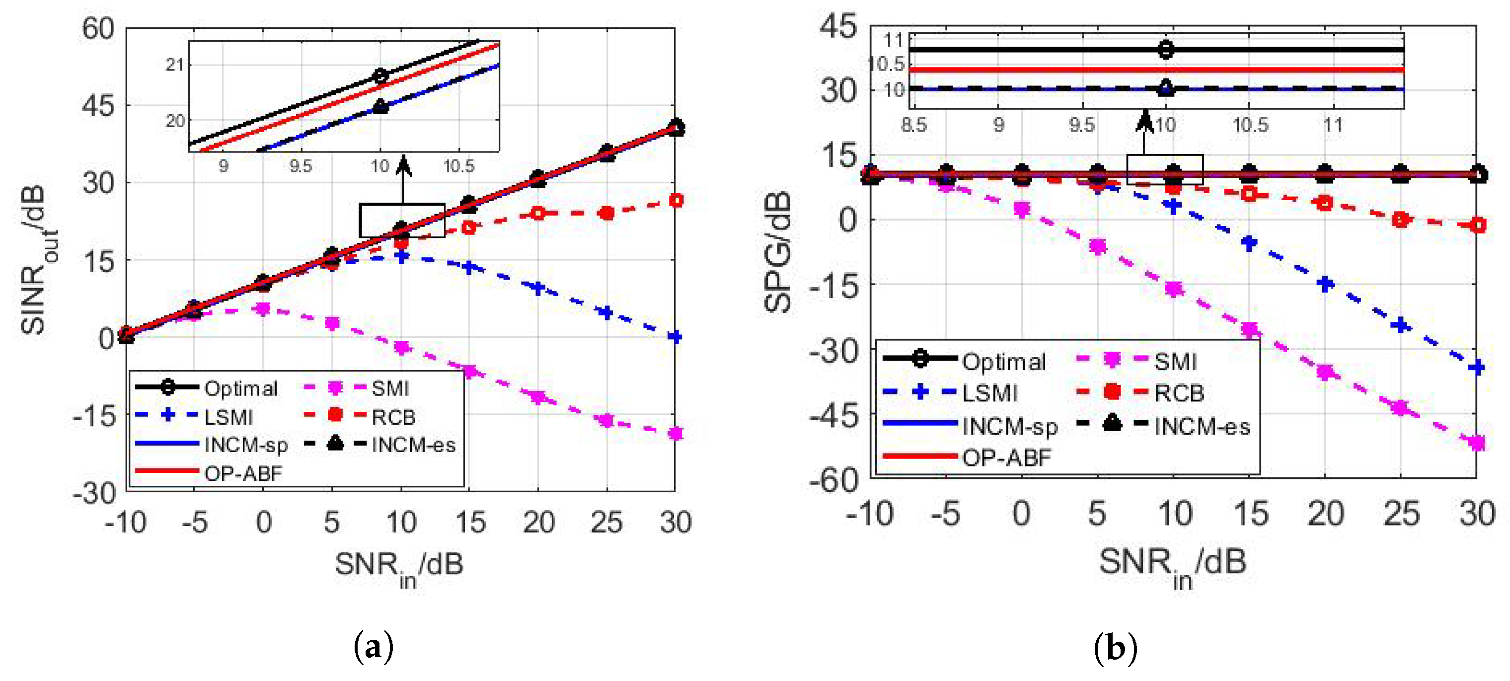
5.1.1. The SINRout and SPG versus the SNRin

In this case, the sample size is fixed to be L = 400. Figure 3 shows the relationship between the SINRout and the SNRin and that between the SPG and the SNRin, respectively.
It can be seen from Figure 3a,b that, except for the SMI, the performance of other algorithms is similar as the mismatch has less impact on the SINRout at low SNRin(≤5 dB). With the increase of the SNRin, the SINRout and the SPG of the SMI decrease seriously. The LSMI and the RCB improve the performance of the SMI to some extent, but both of them are DL methods [12] and cannot eliminate the SV mismatch. The mismatch is amplified as the SNRin increases, so their SPGs start to decline significantly at 10 dB and 20 dB, respectively, as shown in Figure 3b. The SINRout and the SPG of the two INCM algorithms and the OP-ABF achieve their own optimal values under each SNRin, respectively, and the OP-ABF is about 1dB closer to the global optimal SINRout ( SNR in + 10 lg M ) than the two INCM algorithms G opt 10 lg M [35], which suggests that the OP-ABF eliminates more mismatch components than the INCM algorithms.

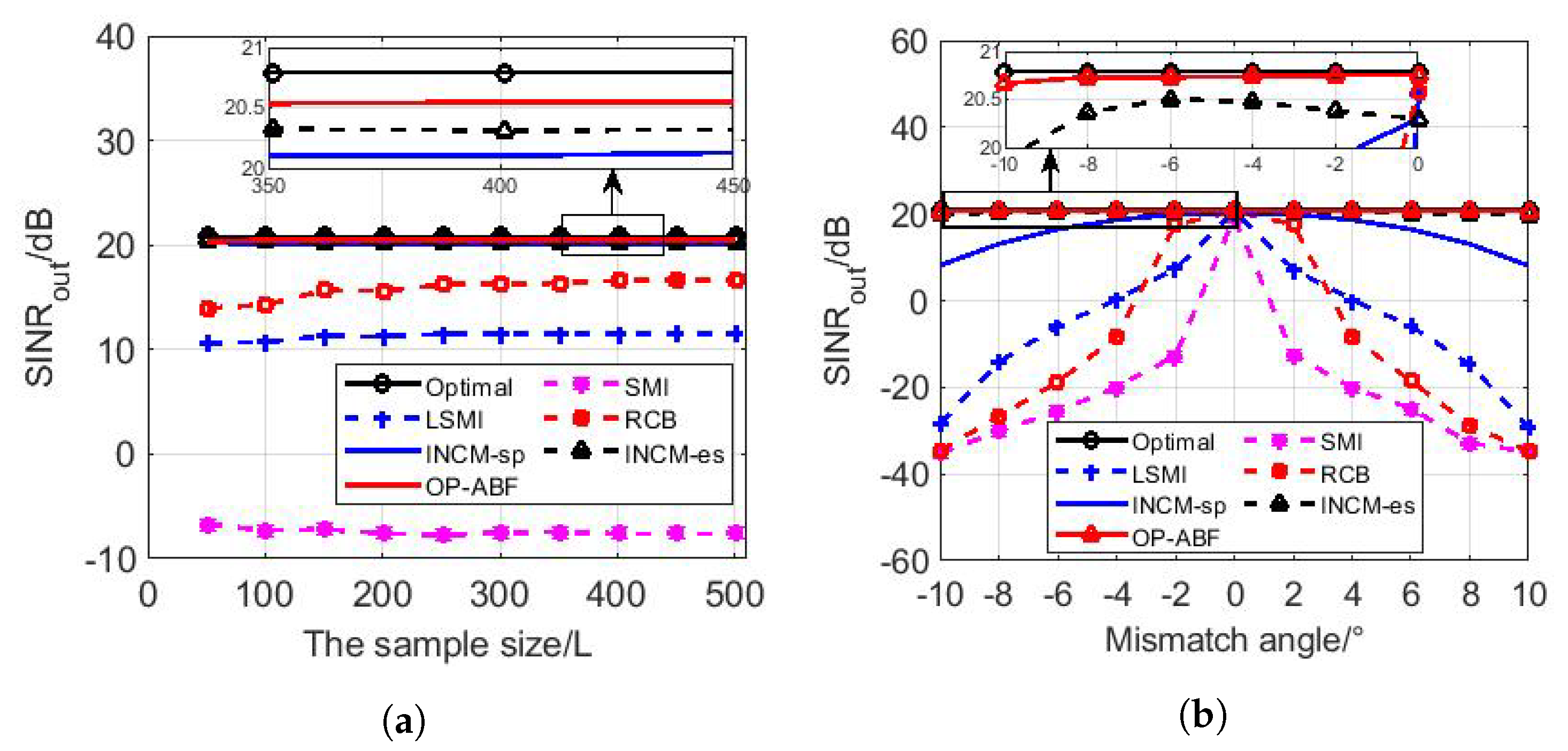
5.1.2. SINRout versus the Sample Size

In this case, the SNR in of each hydrophone is fixed at 10 dB. Figure 4a demonstrates the convergence rates of different algorithms when they achieve their own optimal SINR out . The SMI has the worst SINR out , while the LSMI and the RCB gradually converge with the increase in the sample size, and their SINR out values finally approximate their maximum values, corresponding to Figure 3a. The other three algorithms converge to their respective SINR out , although the sample size is small (L < 200), in which the OP-ABF is closest to the optimal SINR out , followed by the two INCM algorithms. The OP-ABF has the best SINR out provided that the minimum number of samples( L 2 M ) [23,39] is satisfied.

5.1.3. SINRout versus Mismatch Angles

In this case, the SNRin and the sample size are fixed at 10 dB and 400, respectively. Assume a direction of arrival mismatch between a 0 and a asv , and that the angular sector of the D.O.A mismatch is [ 10 , 10 ] [40].
As shown in Figure 4b, the SINRout of the SMI, the LSMI, and the RCB decrease with the increase in angle mismatch, indicating that these three algorithms are sensitive to the D.O.A mismatch, while the SINRout of the INCM-sp does not degrade as severely as those of the previously mentioned three algorithms (10 dB lower than the optimal value at worst), and the SINRout of the INCM-es is slightly lower than the optimal one. In particular, the SINRout degradation is not more than 0.5 dB when the D.O.A mismatch exceeds 8°. In other words, the SINRout of the OP-ABF basically does not change with the D.O.A mismatch, mainly due to the OP-ABF estimates a asv caused by constructing an angular sector, and the change in a asv within this sector does not affect the SINRout of the OP-ABF.

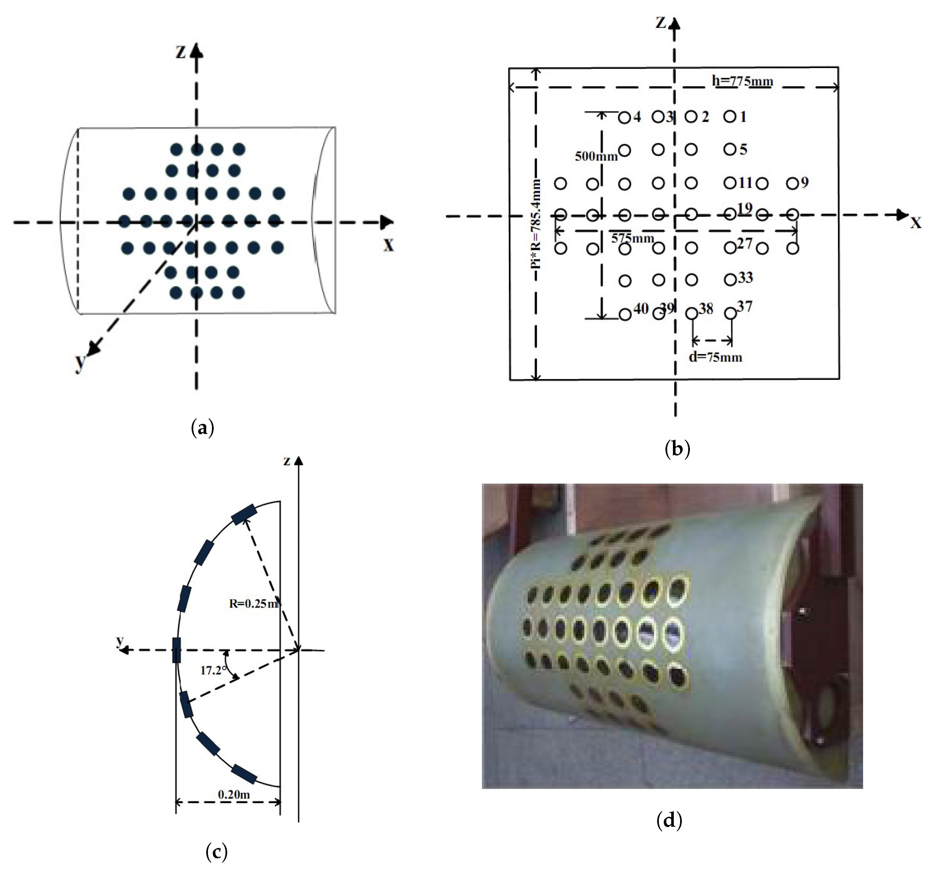
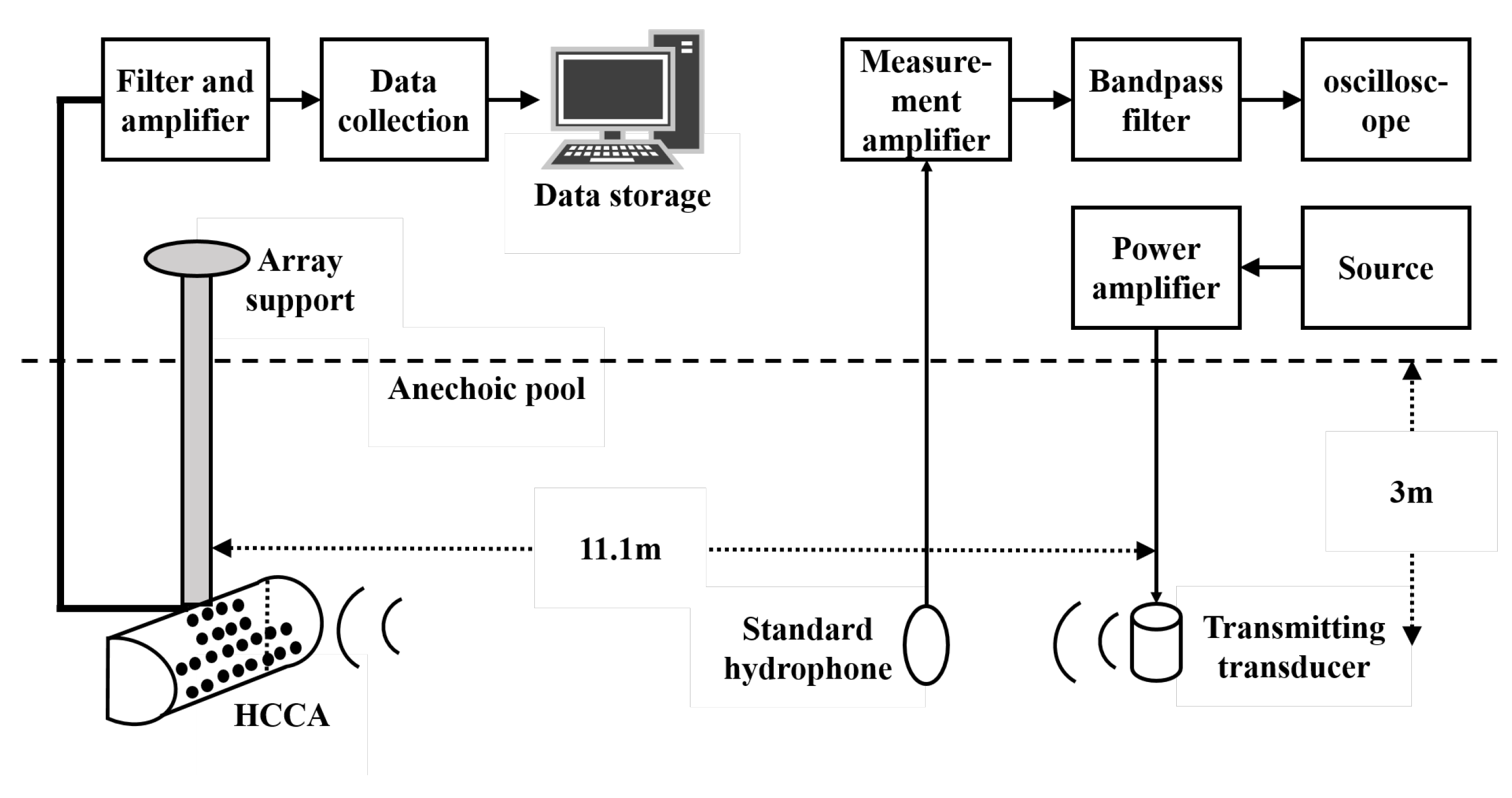
5.2. The Results on HCCA

The geometry and parameters of the conformal array are shown in Figure 5. A table (Table 2) was drawn to supply the relevant parameters of the HCCA shown in Figure 5d. The a asv was obtained by the finite-element software COMSOL [41] to guarantee the model in practice [9], which converts the physical model into the finite element mesh model, and then carries out the numerical calculation.

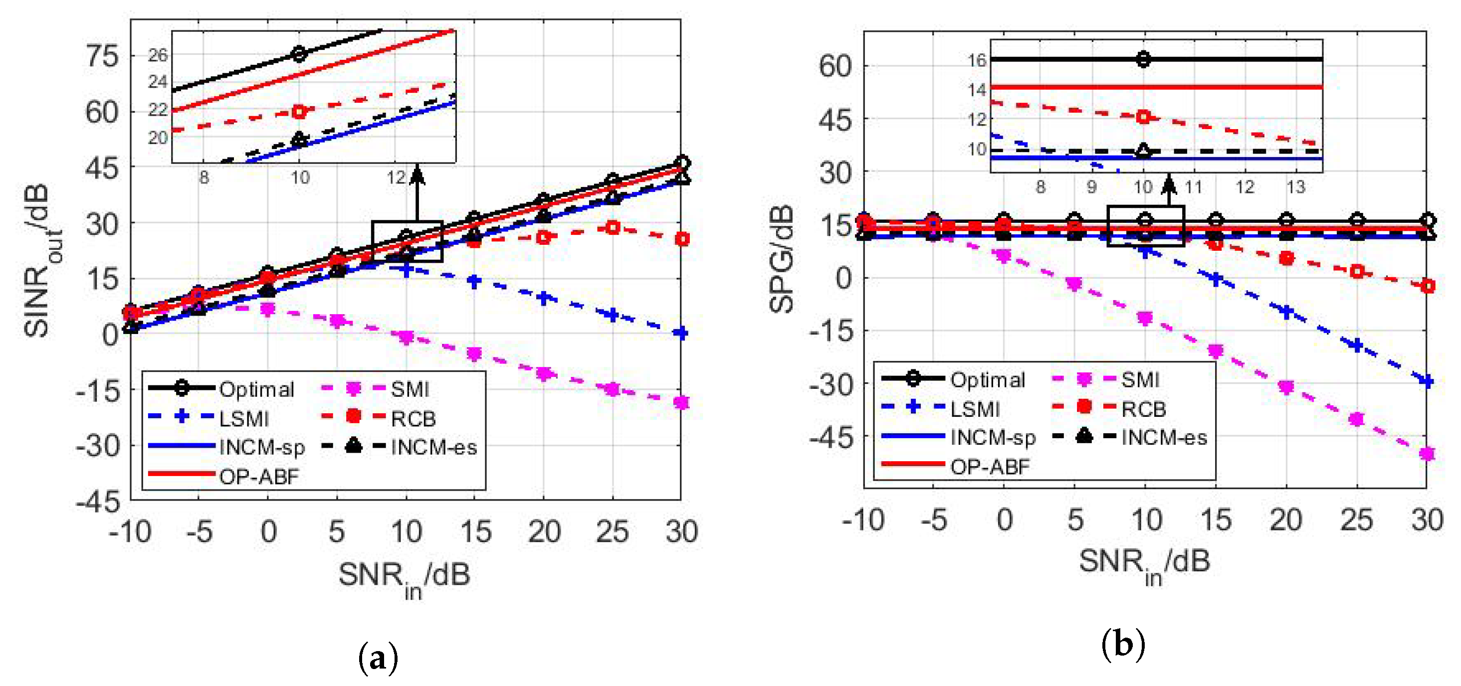
5.2.1. The SINRout and SPG versus the SNRin

The parameter settings are the same as Section 5.1.1 Regardless of the SINRout or the SPG in Figure 6a or Figure 6b, the performance curves of the SMI, the LSMI, and the RCB are consistent with their own, as shown in Figure 3. The SINRout and the SPG of the two INCMs and the OP-ABF keep the same trend as the optimal; the difference is that the performance of these INCMs is always 3 dB–4 dB lower than that of the optimal, and that of the OP-ABF is the closest to that of the optimal drop of no more than 2 dB because the OP operator can eliminate the SV mismatch no matter the type of mismatch, while the other methods do not perform well for the mismatch caused by scattering effects. As a result, the SPG of the OP-ABF is the highest compared with other algorithms.

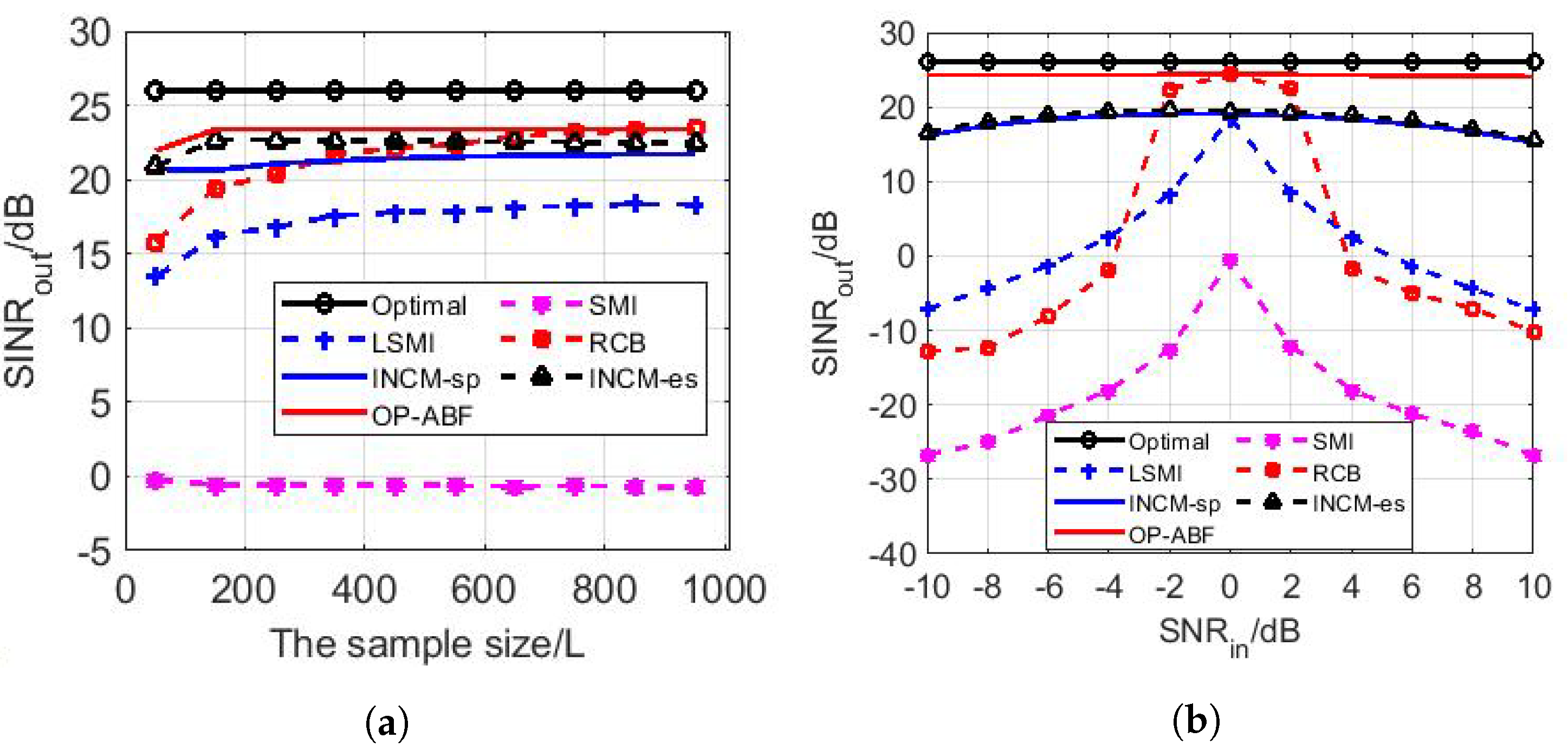
5.2.2. SINRout versus the Sample Size

In this case, the SNRin of each hydrophone is set the same as Section 5.1.2 In addition to the similar phenomenon as Figure 4a, it can be observed in Figure 7a that, when L 2 M , the SINRout of the INCM-sp, the INCM-es, and the OP-ABF are distinctly lower than those of their respective converged values. Then, their SINRout eventually reach their maximum values with L increasing by 800. There are two main reasons for this phenomenon: first, the converged number of samples required here is higher than that of the ULA because more hydrophones are used than ULAs. The second is that the scattering effect increases the convergence threshold of beamformers.

5.2.3. SINRout versus Mismatch Angles
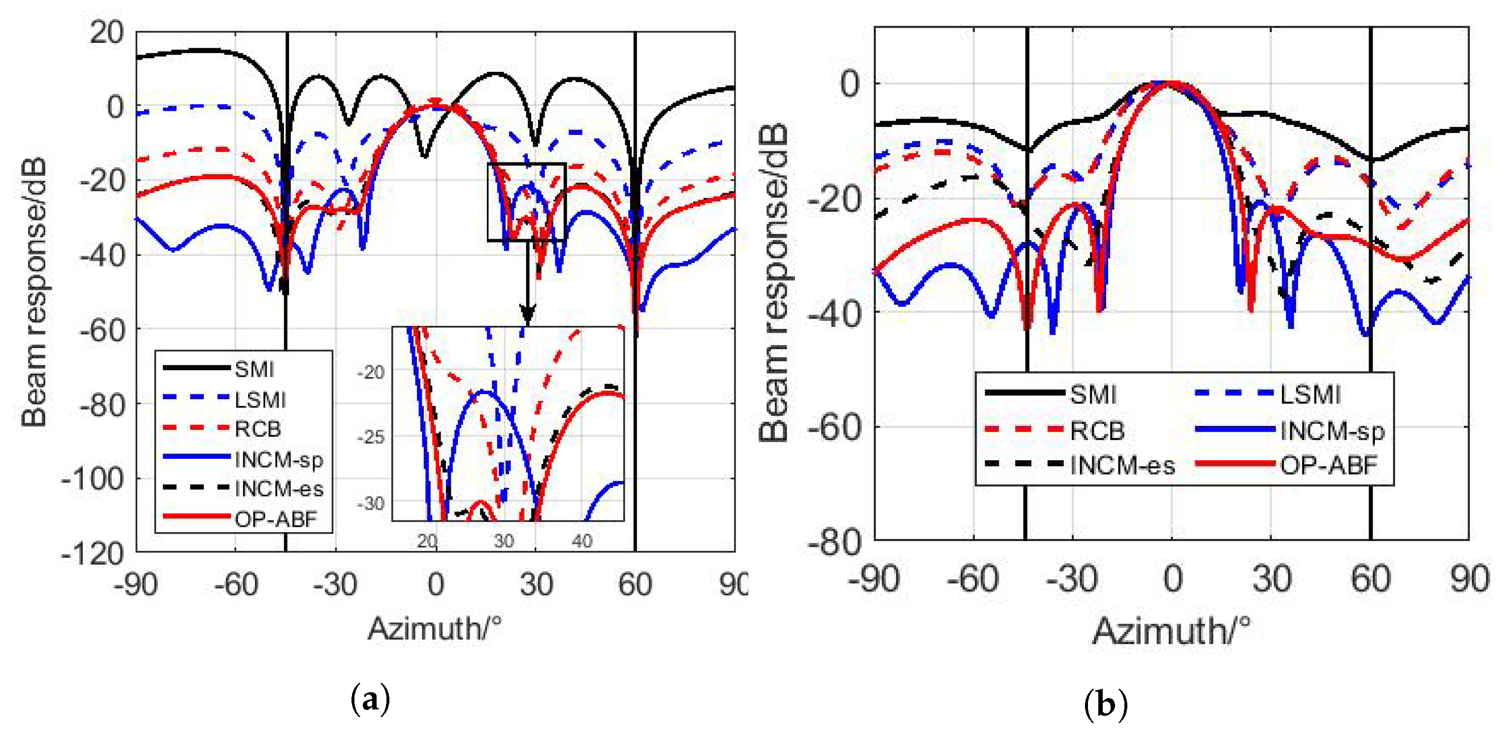
In this case, the SNRin and the sample size are set as Section 5.1.3. The only difference with Section 5.1.3 is that here, a asv , including the component scattered by a rigid baffle, is adopted by using COMSOL. As shown in Figure 7b, one obvious difference is that the INCM-es with the HCCA is less sensitive to the D.O.A mismatch than that with the ULA, as shown in Figure 4b. Similarly, the SINRout of the OP-ABF maintains the optimal result compared to all other algorithms; the reason for this is analyzed in Section 5.1.3.

5.2.4. Beampatterns

In this case, the SNRin and the sample size are the same as those in Section 5.2.3. In Figure 8a, both beampatterns of the SMI and the LSMI show the signal self-nulling phenomenon [42] in the vicinity of the direction of the desired signal, which results in their SINRout degradation. Although the beampattern of the INCM-sp has a narrower mainlobe bandwidth than that of the RCB, the interference at −45° is not perfectly suppressed by the INCM-sp. Fortunately, the OP-ABF accurately suppresses all interferences, while it maintains its overall performance, and its sidelobe level is slightly lower than that of the INCM-es.
The results in Figure 8a confirm the evaluations of various methods in the above: the DL beamformers cannot completely eliminate the SV mismatch, the INCM algorithms retain some of the mismatch component, and the OP-ABF eliminates the mismatch while ensuring the interference suppression of the beamformer.
Figure 8b illustrates beampatterns of different algorithms using experimental data, which are derived from an experiment in the anechoic pool. The schematic diagram of the experimental environment and instrument arrangement are given in Figure 9, in which the information on each instrument is listed in the Table 3. The source adopts a continuous wave (CW) pulse and the duration of the pulse is reasonably designed. It transmits a single-frequency signal whose frequency is 10 kHz, and the sampling frequency is 48 kHz. The source and the HCCA are on the same plane. The format of the experimental data collected by the HCCA is converted and then we input it to MATLAB to obtain the results on beamforming. The SVs of the desired signal and interferences are obtained through experimental measurement. These SVs are not only affected by the SV mismatch mentioned in this paper, but also affected by the experimental errors.
In Figure 8b, only the OP-ABF and the INCM-sp can maintain a performance close to those in the simulation, while the other three suffer from serious performance degradation. Interestingly, the beampattern of the INCM-sp in Figure 8b loses the interference suppression with its performance close to that of the CBF, whereas there is only a null for the interference at 45° by the OP-ABF. We think the signal incident from the endfire direction has low power due to the block of the rigid baffle and is submerged in noise, while the preservation of the mainlobe proves that the OP-ABF is robust in eliminating the SV mismatch of the desired signal. The results of the experimental data are in agreement with the simulated ones, which verifies the effectiveness of the OP-ABF algorithm.

6. Conclusions

In this paper, a novel algorithm of adaptive beamforming based on OP (OP-ABF) was proposed to solve the SV mismatch of hydrophone arrays. This algorithm originates from the introduction of the OP operator to the analytical expression of the SMI weight vector, and application of the OPMCV to compensate for the SV mismatch. Then, the indispensable parameters in the OPMCV were estimated, the OP matrix was derived, and the remaining parameters were optimized under the CML framework. Finally, in the case of the SV mismatch, the effectiveness of the proposed OP-ABF was verified by simulation and experimental data using two different geometric arrays. The OP-ABF can not only eliminate the arbitrary-type of SV mismatch, but also improves the beamforming performance without using too much information in the received data. The simulations of the ULA show that the OP-ABF can obtain the highest SINRout under different conditions compared with other algorithms introduced in this paper. In particular, the OP-ABF can not only eliminate the SV mismatch caused by the scattering of the rigid baffle of the conformal arrays, but also maintain a high SINRout with the help of COMSOL and experimental data, which indicates that OP-ABF has broad application prospects on various underwater platforms. For example, the OP-ABF can be simultaneously applied to multiple arrays of the unmanned underwater vehicle (UUV) to realize combined data processing. In addition, the OP-ABF shows significant performance in underwater interference suppression by eliminating the SV mismatch.
There are various avenues for the future work to be explored. For example, it would be interesting for conformal arrays to extend our proposed algorithm to two-dimensional space. This would provide them with an advantage over towed linear arrays. Alternatively, an important issue, falling slightly beyond the scope of the current work, is to extend our results to produce D.O.A methods and to analyze their performance, such as robustness, resolution, etc.

Author Contributions

Conceptualization, Y.D.; methodology, Y.D. and C.S.; validation, Y.D.; formal analysis, Y.D.; investigation, Y.D.; resources, C.S.; data curation, Y.D.; writing—original draft preparation, Y.D.; writing—review and editing, C.S.; supervision, C.S.; project administration, C.S.; funding acquisition, C.S. All authors have read and agreed to the published version of the manuscript.

Funding

This research received no external funding.

Institutional Review Board Statement

Not applicable.

Informed Consent Statement

Not applicable.

Data Availability Statement

The data presented in this study are available on request from the corresponding author.

Conflicts of Interest

The authors declare no conflict of interest.

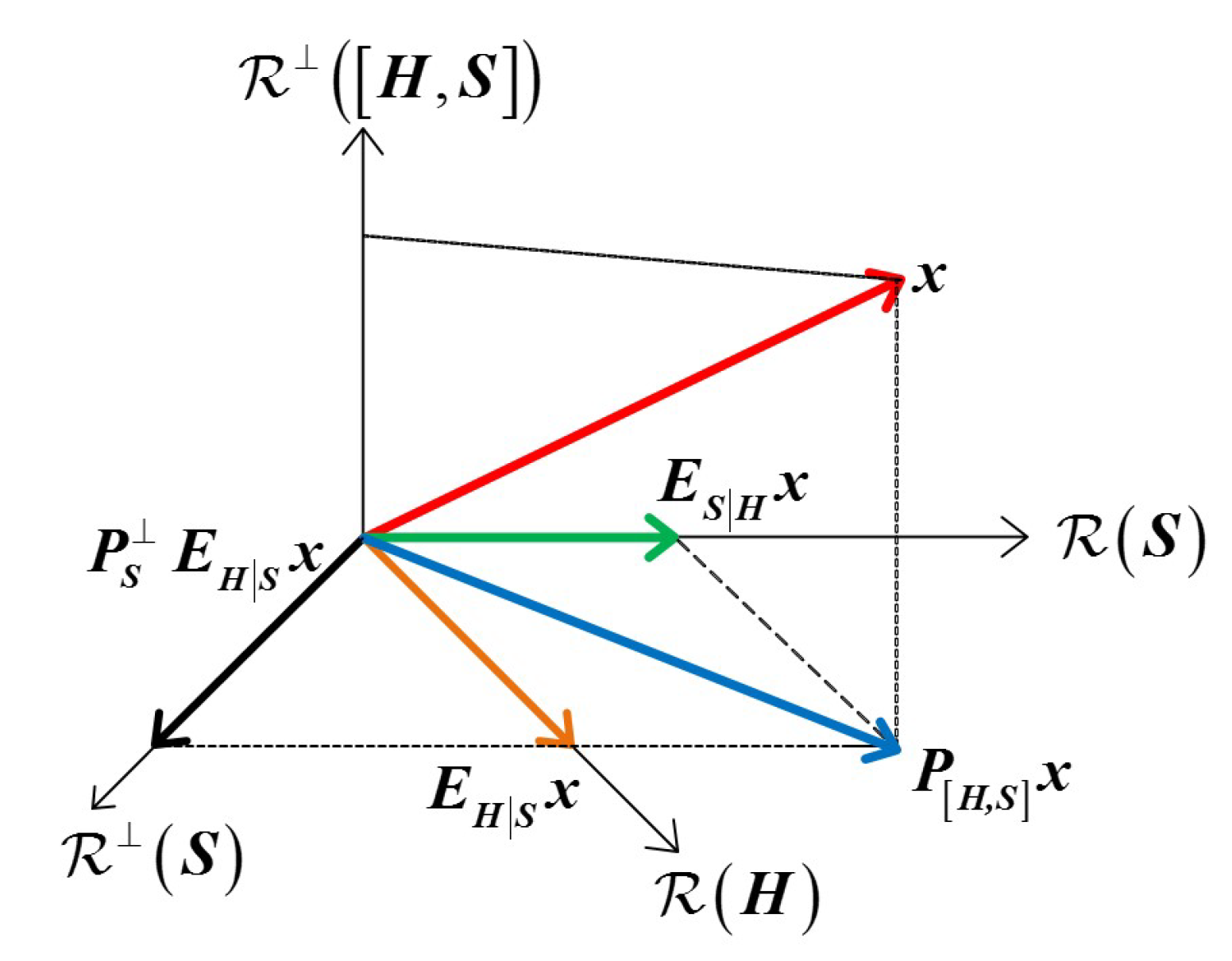
Appendix A. Oblique Projection

Now consider a n × m + k matrix [ H , S ] composed of two full column rank matrices H C n × m and S C n × k , where m + k < n , and R H is linearly independent of R S , so there is disjointness between R H and R S .
According to the definition, the orthogonal projection matrix to R H , S is
P HS = H , S H H H H H S S H S S H S 1 H H S H
and P HS can be rewritten as
P HS = E H S + E S H
where
E H S = H H H P S H 1 H H P S
and
E S H = S S H P H S 1 S H P H
are known as oblique projection (OP) operators, where P H = I P H and P S = I P S correspond to R H and R S , respectively.
It can be seen from (A3) and (A4) that E H S and E S H are idempotent but not Hermitian. Such matrices have the following properties:
E H S H = H , E H S S = 0 E S H S = S , E S H H = 0
The geometric relationship between E H S and E S H is shown in Figure A1, in which E H S is the oblique projector onto R H along the direction parallel to R S , and E S H is the oblique projector onto R S along the direction parallel to R H .
Figure A1. Geometric interpretation of oblique projection.
Jmse 11 00876 g0a1

References

  1. Nielsen, R.O. Sonar Signal Processing; Artech House: Boston, MA, USA, 1991; ISBN 978-0890064535. [Google Scholar]
  2. Knight, W.C.; Pridham, R.G.; Kay, S.M. Digital Signal Processing for Sonar. Proc. IEEE 1981, 69, 1451–1506. [Google Scholar] [CrossRef]
  3. Vaccaro, R.J. The past, present, and the future of underwater acoustic signal processing. IEEE Signal Process. Mag. 1998, 15, 21–51. [Google Scholar] [CrossRef]
  4. Baggeroer, A.B. Sonar arrays and array processing. AIP Conf. Proc. 2005, 760, 3–24. [Google Scholar] [CrossRef]
  5. Li, Q.H. Digital Sonar Design in Underwater Acoustics: Principles and Applications; Zhejiang University Press: Hangzhou, China; Springer: Berlin/Heidelberg, Germany, 2011. [Google Scholar] [CrossRef]
  6. Capon, J. High-resolution frequency-wavenumber spectrum analysis. Proc. IEEE 1969, 57, 1408–1418. [Google Scholar] [CrossRef]
  7. Huang, L.; Zhang, J.; Xu, X.; Ye, Z. Robust Adaptive Beamforming with a Novel Interference-Plus-Noise Covariance Matrix Reconstruction Method. IEEE Trans. Signal Process. 2015, 63, 1643–1650. [Google Scholar] [CrossRef]
  8. Gershman, A.B.; Turchin, V.I.; Zverev, V.A. Experimental results of localization of moving underwater signal by adaptive beamforming. IEEE Trans. Signal Process. 1995, 43, 2249–2257. [Google Scholar] [CrossRef]
  9. Yang, B.; Sun, C.; Chen, Y.L. Conformal Array Beampattern Optimization Method and Experimental Research Based on Sound Field Forecast. Torpedo Technol. 2006, 14, 18–20, 60. Available online: https://en.cnki.com.cn/Article_en/CJFDTotal-YLJS200601003.htm (accessed on 26 March 2023).
  10. Wax, M.; Anu, Y. Performance analysis of the minimum variance beamformer. IEEE Trans. Signal Process. 1996, 44, 928–937. [Google Scholar] [CrossRef]
  11. Cox, H. Resolving power and sensitivity to mismatch of optimum array processors. J. Acoust. Soc. Am. 1973, 54, 771–785. [Google Scholar] [CrossRef]
  12. Yan, S.F. Optimal Array Signal Processing: Beamforming Design Theory and Methods; Science Press: Beijing, China, 2018; ISBN 978-7-03-043964-2. [Google Scholar]
  13. Cox, H.; Zeskind, R.; Owen, M. Robust adaptive beamforming. IEEE Trans. Acoust. Speech Signal Process. 1987, 35, 1365–1376. [Google Scholar] [CrossRef]
  14. Jian, L.; Stoica, P.; Wang, Z.S. On robust capon beamforming and diagonal loading. IEEE Trans. Signal Process. 2003, 51, 1702–1715. [Google Scholar] [CrossRef]
  15. Vorobyov, S.A. Principles of minimum variance robust adaptive beamforming design. Signal Process. 2013, 93, 3264–3277. [Google Scholar] [CrossRef]
  16. Malioutov, D.; Cetin, M.; Willsky, A.S. A sparse signal reconstruction perspective for source localization with sensor arrays. IEEE Trans. Signal Process. 2005, 53, 3010–3022. [Google Scholar] [CrossRef]
  17. Gu, Y.; Goodman, N.A.; Hong, S.; Li, Y. Robust adaptive beamforming based on interference covariance matrix sparse reconstruction. Signal Process. 2014, 96, 375–381. [Google Scholar] [CrossRef]
  18. Wang, H.; Ma, Q.M. A robust adaptive beamforming algorithm based on covariance matrix reconstruction. Acta Acust. 2019, 44, 170–176. [Google Scholar] [CrossRef]
  19. Shen, F.; Chen, F.F.; Song, J.Y. Robust adaptive beamforming based on steering vector estimation and covariance matrix reconstruction. IEEE Commun. Lett. 2015, 19, 1636–1639. [Google Scholar] [CrossRef]
  20. Yuan, X.L.; Gan, L. Robust adaptive beamforming via a novel subspace method for interference covariance matrix reconstruction. Signal Process. 2017, 130, 233–242. [Google Scholar] [CrossRef]
  21. Yang, J.; Yang, Y.; Lei, B. An efficient robust adaptive beamforming method using steering vector estimation and interference covariance matrix reconstruction. In Proceedings of the 2018 OCEANS-MTS/IEEE Kobe Techno-Ocean (OTO), Kobe, Japan, 28–31 May 2018. [Google Scholar] [CrossRef]
  22. Chen, P.; Yang, Y.X.; Wang, Y.; Ma, Y.L.; Yang, L. Robust covariance matrix reconstruction algorithm for time-domain wideband adaptive beamforming. IEEE Trans. Veh. Technol. 2019, 68, 1405–1416. [Google Scholar] [CrossRef]
  23. Feldman, D.D.; Griffiths, L.J. A projection approach for robust adaptive beamforming. IEEE Trans. Signal Process. 1994, 42, 867–876. [Google Scholar] [CrossRef]
  24. Biguesh, M.; Valaee, S.; Champagne, B.; Bastani, M.H. A new beamforming algorithm based on signal subspace eigenvectors. In Proceedings of the Tenth IEEE Workshop on Statistical Signal and Array Processing (Cat. No.00TH8496), Pocono Manor, PA, USA, 16 August 2000. [Google Scholar] [CrossRef]
  25. Chang, A.C.; Chiang, C.T.; Chen, Y.H. A generalized eigenspace-based beamformer with robust capabilities. In Proceedings of the IEEE International Conference on Phased Array Systems and Technology, (Cat. No.00TH8510), Dana Point, CA, USA, 21–25 May 2000. [Google Scholar] [CrossRef]
  26. Yi, S.C.; Ying, W.; Wang, Y.L. Projection-based robust adaptive beamforming with quadratic constraint. Signal Process. 2016, 122, 65–74. [Google Scholar] [CrossRef]
  27. Zhang, X.D. Matrix Analysis and Applications, 2nd ed.; Tsinghua University Press: Beijing, China, 2013. [Google Scholar] [CrossRef]
  28. Behrens, R.T.; Scharf, L.L. Signal processing applications of oblique projection operators. IEEE Trans. Signal Process. 1994, 42, 1413–1424. [Google Scholar] [CrossRef]
  29. Yang, X.P.; Zhang, Z.A.; Zheng, T.; Long, T.; Sarkar, T.K. Mainlobe interference suppression based on eigen-projection processing and covariance matrix reconstruction. IEEE Antennas Wirel. Propag. Lett. 2014, 13, 1369–1372. [Google Scholar] [CrossRef]
  30. Guo, X.L.; Li, X.Y.; Qiu, W. A mainlobe jamming suppression method based on spatial spectrum estimation oblique projection filtering in beam space. Radar Sci. Technol. 2019, 17, 329–334. [Google Scholar] [CrossRef]
  31. Zhang, X.J.; He, Z.S.; Liao, B.; Zhang, X.P.; Yang, Y. Pattern synthesis via oblique projection based multi-point array response control. IEEE Trans. Antennas Propag. 2019, 67, 4602–4616. [Google Scholar] [CrossRef]
  32. Zhang, X.J.; He, Z.S.; Liao, B.; Yang, Y.; Zhang, J.F. Flexible array response control via oblique projection. IEEE Trans. Signal Process. 2019, 67, 3126–3139. [Google Scholar] [CrossRef]
  33. Wax, M.; Adler, A. Subspace-constrained array response estimation in the presence of model errors. IEEE Trans. Signal Process. 2021, 69, 417–427. [Google Scholar] [CrossRef]
  34. Zhang, X.; He, Z.; Xia, X.G.; Liao, B.; Zhang, X.; Yang, Y. OPARC: Optimal and precise array response control algorithm-part II: Multipoints and applications. IEEE Trans. Signal Process. 2019, 67, 668–683. [Google Scholar] [CrossRef]
  35. Van Trees, H.L. Optimum Array Processing: Part IV of Detection, Estimation, and Modulation Theory; John Wiley & Sons Ltd.: New York, NY, USA, 2002. [Google Scholar] [CrossRef]
  36. Grant, M.C.; Boyd, S.P. The CVX Users’ Guide, Release 2.2; CVX Research, Inc.: Austin, TX, USA, 2020; Available online: http://cvxr.com/cvx (accessed on 27 March 2023).
  37. Vorobyov, S.A.; Gershman, A.B.; Luo, Z.Q. Robust adaptive beamforming using worst-case performance optimization via Second-Order Cone programming. In Proceedings of the 2002 IEEE International Conference on Acoustics, Speech, and Signal Processing, Orlando, FL, USA, 13–17 May 2002. [Google Scholar] [CrossRef]
  38. Valaee, S.; Champagne, B.; Kabal, P. Parametric localization of distributed sources. IEEE Trans. Signal Process. 1995, 43, 2144–2153. [Google Scholar] [CrossRef]
  39. Reed, I.S.; Mallett, J.D.; Brennan, L.E. Rapid Convergence Rate in Adaptive Arrays. IEEE Trans. Aerosp. Electron. Syst. 1974, 10, 853–863. [Google Scholar] [CrossRef]
  40. Yu, Z.L.; Ser, W.; Er, M.H.; Gu, Z.; Li, Y. Robust Adaptive Beamformers Based on Worst-Case Optimization and Constraints on Magnitude Response. IEEE Trans. Signal Process. 2009, 57, 2615–2628. [Google Scholar] [CrossRef]
  41. COMSOL Multiphysics® v.5.2. Acoustics Module Users’ Guide; COMSOL AB: Stockholm, Sweden, 2021. Available online: https://cn.comsol.com/models/acoustics-module (accessed on 8 April 2023).
  42. Widrow, B.; Duvall, K.; Gooch, R.; Newman, W. Signal cancellation phenomena in adaptive antennas: Causes and cures. IEEE Trans. Antennas Propag. 1982, 30, 469–478. [Google Scholar] [CrossRef]
Figure 1. Diagram of the geometric interpretation of (17), in which the red arrow represents the minimum variance distortionless response (MVDR) beamformer, and the blue arrow is the sample matrix inversion (SMI) beamformer. When a asv a 0 , the two beamformers are no longer linearly correlated because of the SV mismatch, and the resulting error is v OPMCV represented by the green arrow. These three vectors can form a vector triangle in linear space.
Jmse 11 00876 g001
Figure 2. Flowchart of the implementation of the OP-ABF. It can be seen from the flowchart that E ^ is calculated by R ^ , and μ α is solved by R ^ and E ^ . Substituting E ^ and μ α into (24), w OP is eventually derived.
Jmse 11 00876 g002
Figure 3. Performance comparison of different algorithms by the uniform linear array (ULA): (a) the output signal-to-interference-plus-noise ratio ( SINR out ) vs. the input signal-to-noise ratio ( SNR in ) and (b) the spatial processing gain (SPG) vs. SNR in .
Jmse 11 00876 g003
Figure 4. Performance comparison of different algorithms by the ULA: (a) SINR out versus the sample size and (b) SINR out versus the direction of arrival (D.O.A) mismatch.
Jmse 11 00876 g004
Figure 5. Diagram of the half-cylindrical conformal array (HCCA) configuration: (a) the three-dimensional (solid black dots represent hydrophones); (b) front view (the top left circle represents the hydrophone number 1, the bottom right circle represents the hydrophone number 40, and the labels of hydrophones increase from top left corner to bottom right corner); (c) side view; (d) the real object.
Jmse 11 00876 g005
Figure 6. Performance comparison of different algorithms by the HCCA: (a) SINR out versus SNR in and (b) the SPG versus SNR in .
Jmse 11 00876 g006
Figure 7. Performance comparison of different algorithms by the HCCA: (a) SINR out versus the sample size and (b) SINR out versus the D.O.A mismatch.
Jmse 11 00876 g007
Figure 8. Beampattens by the HCCA: (a) simulation data and (b) experiment data.
Jmse 11 00876 g008
Figure 9. Schematic diagram of the experimental environment and the instruments arrangement. The receiving module is on the left and the transmitting one is on the right.
Jmse 11 00876 g009
Table 1. Proposed Adaptive Beamforming Algorithm Based on Oblique Projection (OP-ABF).
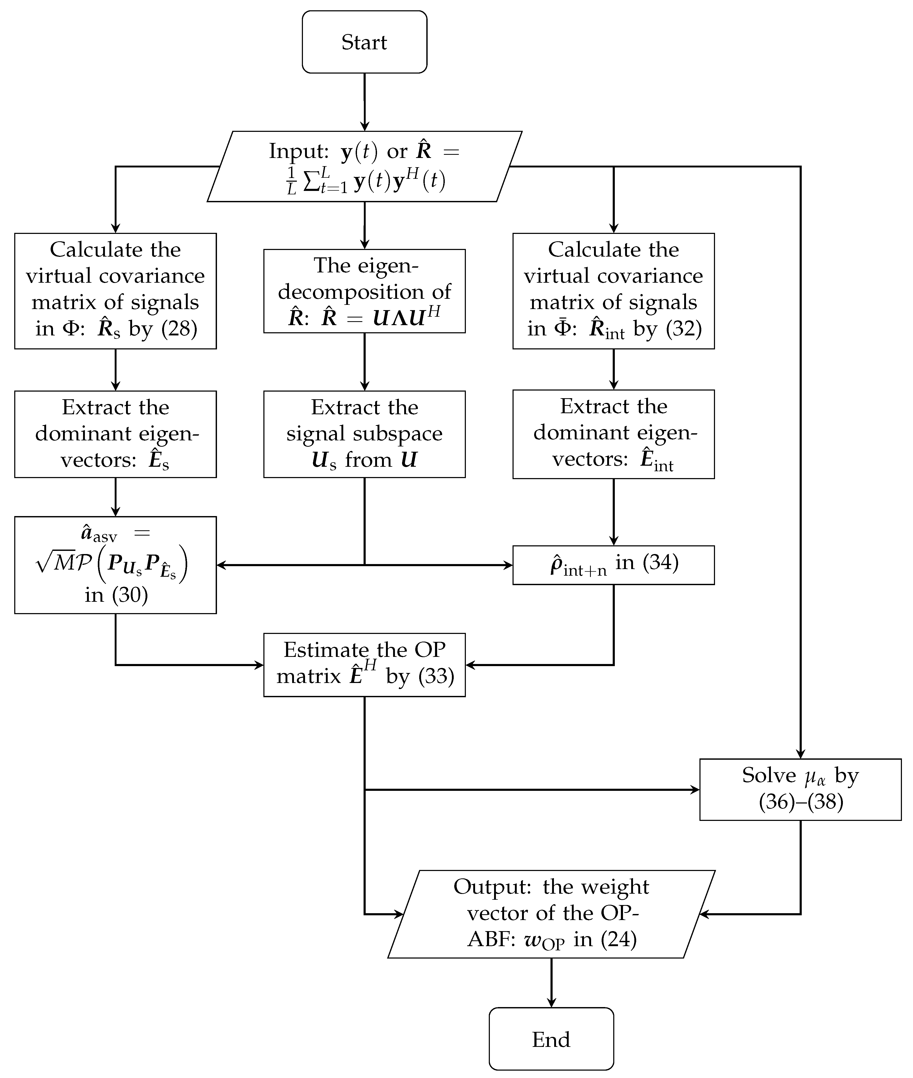
step1: Obtain the eigen-subspaces corresponding to the dominant eigenvalues of R ^ in (3), R ^ s in (28) and R ^ int + n in (32) by eigen-decomposition, respectively.
step2: Substitute (30), (31), and (34) into (33). The OP matrix and the actual SV of the desired signal are estimated by E ^ and a ^ asv , respectively.
step3: Solve the optimization problem (36), and obtain the solution of μ α in (38).
step4: Substitute E ^ , a ^ asv and μ α into (24) and obtain w OP .
Table 2. The physical parameters of the HCCA in Figure 5.
The Length of the Bus BarThe RadiusThe Number of HydrophonesThe Spacing between HydrophonesThe Operating Frequency
h = 0.775 mr = 0.25 m40d = 0.075 m6 kHz–10 kHz
Table 3. The information on hardware in the experiment.
TransmissionReception
InstrumentsInformationInstrumentsInformation
SourceRIGOL DG1000
function/arbitrary
waveform generator
Conformal arrayHCCA shown in
Figure 5 and Table 2
Power amplifierL6 linear
power amplifier
Transmitting
Transducer
Overflow ringFilter and amplifierPF28000 Cut-off frequency:
Operating frequency:
8 kHz–10 kHz
1 Hz–3.15 MHz
OscilloscopeInfiniiVision 2000 X Maximum gain
 multiplier: 8192
Bandpass filterPF-1U Filter Channels: 64
Cut-off frequency:
204.6 kHz
Data collectionSampling frequency:
32 kHz–96 Hz
Maximum gain
multiplier: 8192
Measurement
amplifier
Conditioning Amplifier
Standard
hydrophone
D/140/HData storageWorkstation
Operating frequency:
10 Hz–200 kHz
Receive sensitivity
(re 1 V/μPa): −193 dB@1 kHz
Disclaimer/Publisher’s Note: The statements, opinions and data contained in all publications are solely those of the individual author(s) and contributor(s) and not of MDPI and/or the editor(s). MDPI and/or the editor(s) disclaim responsibility for any injury to people or property resulting from any ideas, methods, instructions or products referred to in the content.

