Application of a Deep Neural Network for Acoustic Source Localization Inside a Cavitation Tunnel

Abstract

Navigating with low noise is the key capability in the submarine design considerations, and noise reduction is also one of the most critical issues in the related fields. Therefore, it is necessary to identify the source of noise during design stage to improve the survivability of the submarines. The main objective of this research is using the supervised neural network to construct the system of noise localization to identify noise source in the large acoustic tunnel. Firstly, we started our proposed method by improving the Yangzhou’s method and Shunsuke’s method. In the test results, we find that the errors of the both can be reduced by using the min-max normalization to highlight the data characteristics of the low amplitude in some frequency. And Yangzhou’s method has higher accuracy than Shunsuke’s method. Then, we reset the diagonal numbers of the cross spectral matrix in Yangzhou’s method to zero and replace mean absolute error to be the loss function for improving the stability of training, and get the most suitable neural network construction for our research. After our optimization, the error decreases from 0.315 m to 0.008 m in cuboid model test. Finally, we apply our method to the cavitation tunnel model. A total of 100 data sets were used for training, 10 sets for verification, and 5 for testing. The average error of the test result is 0.13 m. For the model test in cavitation tunnel in National Taiwan Ocean University, the length of ship model is around 7 m. And the average error is sufficient to determine the noise source position.

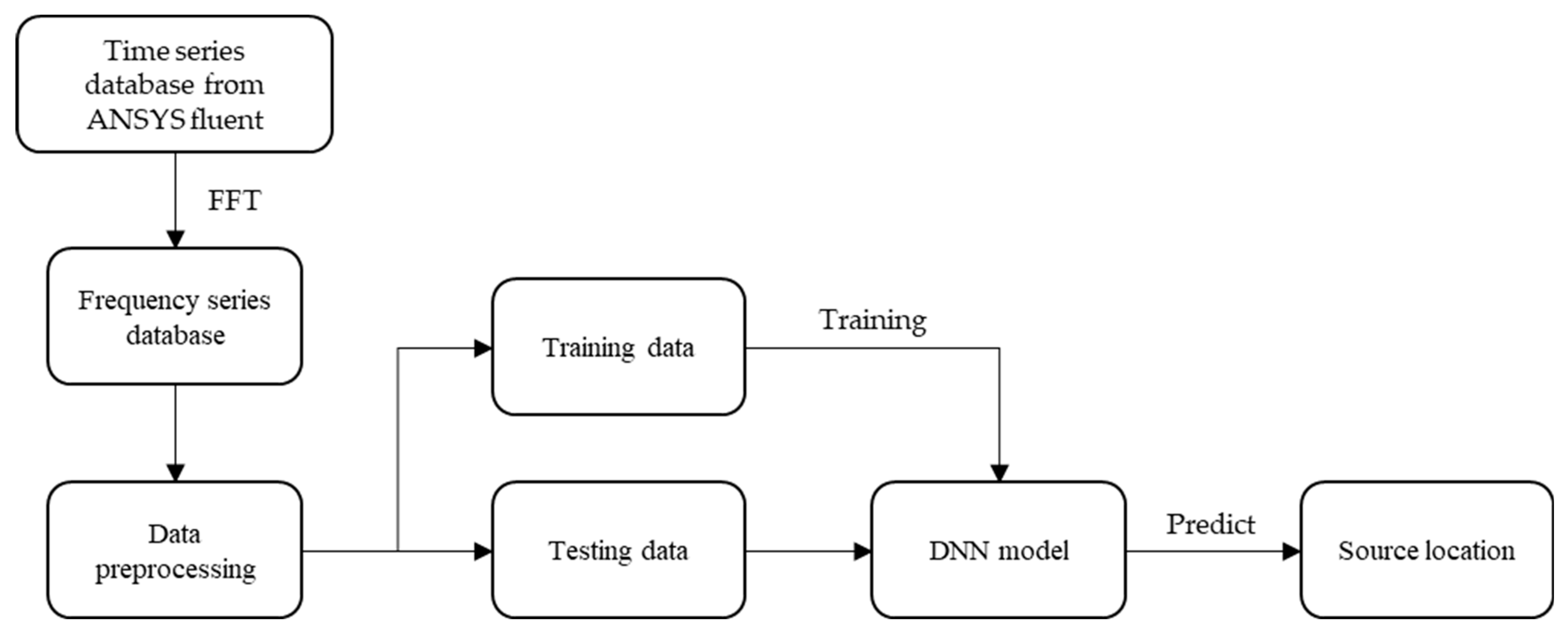
1. Introduction

The difficulty of underwater acoustic, when compared to the air acoustics, is that the transmission of sound in water will be affected more severely by complex environmental factors such as water flow, medium density, viscosity, temperature, wave scattering, and reflection. Many researchers have contributed to the underwater sound source localization problems. Skarsoulis et al. [1] first employed Bayesian method, which uses the phase difference of hydrophone array, to measure the location of two sound sources in the open region with different depths (160 and 1500 m). The frequency of the sound signal is 11.2 kHz. Other researches also applied the machine learning and neural network [2,3,4] to find 400 Hz sound signal in the open water domain.

Additionally, when the sound source localization within a confined space is considered, the strong reflection will make the wave transmission path more complex and difficult to perform the inverse calculation. This makes noise localization very difficult to perform in regular experimental tanks. In 2015, Kim et al. [5] used two parallel moving hydrophone arrays to locate a 20 kHz sound source in 50 m × 35 m × 3.2 m water tank. In 2016, Liu et al. [6] used the passive time-reversal mirror combined with acoustic ray theory to identify a 3–7 kHz sound source within a 165 × 8 × 4 m towing tank. In 2021, Liu et al. [7] used optical fibers to construct sensor array to improve the accuracy. Another issue is that in most cavitation tunnels, the size of the observation device approaching the wave-length of low frequency waves [8]. Some of the existing methods relied on the time difference of the first arriving wave front, which may not be applicable for most experiment required the steady state measurement. The other methods cannot deal with wave frequency lower than 1 kHz because the associated wave length is larger than the size of the hydrophone array or even the size of water tank. However, the target sound source has much lower frequency range. So the phase difference between different measuring device (hydrophone) is approaching the scale of measuring error. These issues make it more difficult to locate the sound source with traditional methods. Therefore, it is a good area for the artificial intelligence (AI) to investigate the nonlinear interaction between the sound source and highly reflective environment.

The development of AI has resulted in machine learning being used in data analysis across various fields, especially when addressing complex problems, such as weather predictions, material crack growth predictions, and detection of underwater acoustic source locations. Many scholars have used machine learning and data generated by acoustic sources to analyze acoustic source locations. Lee et al. [9] performed principal component analysis [10], which is commonly used in statistics, to estimate the locations of high-frequency acoustic sources in a semi-open tank. They first centralized the signal samples at each time point and then decomposed the eigenvalues in the covariance matrices of the centralized samples. Next, several eigenvectors with a large eigenvalue were used to form a matrix through which the centralized samples were projected to generate feature data. The probabilities of the feature data appearing at sample acoustic source locations were used to calculate the weights of the linear regression, thereby allowing the locations of unknown acoustic sources to be predicted. Lefort et al. [11] used nonlinear regression to detect the locations of high-frequency acoustic sources in semi-open water tanks. They established a nonlinear regression model by using kernel regression [12] and adopted L-nearest-neighbor-based approximation [13] to approximate the kernel regression model and reduce the amount of calculations involved. In the aforementioned method, only Euclidean distances must be calculated from the training data, and no training steps are required to determine the locations of acoustic sources. This simple regression analysis method has expanded the basic application of machine learning.

Compared with general machine learning, neural networks are more suitable for nonlinear problems which like sound source localization problem. Vera-Diaz et al. [14] used a convolutional neural network to determine acoustic source locations in fully enclosed spaces in air. They divided each audio source signal by using window functions, processed the signals using one-dimensional-convolution finite impulse response filters, form the signals into a time-domain signal matrix, and then used max pooling layers to extract the characteristics of the signal matrix and inversely calculated acoustic source locations. Although Vera-Diaz et al. ignored signal reverberation and ambient background noise and used air as the ambient medium, their results are still valuable to the present study. Yangzhou et al. [15] divided time-domain data into different segments and implemented the fast Fourier transform (FFT) [16] on them. They set the real and imaginary parts of the transformed frequency-domain data as the input data features for predicting acoustic source locations in enclosed two-dimensional spaces in air. Zhu et al. [17] divided signal data and implemented the FFT to get the training data. They processed the data by conducting principal-component-regression-based feature selection and used a convolutional autoencoder [18] to construct neural network input layers. Next, they trained a problem-solving model by using encoder multilayer perceptron. Feature selection greatly reduced model training time while maintaining considerable accuracy. The focus of the training was on the acoustic source range, and the waters near San Diego ware selected as the experimental site because they resembled a water tank in the open space. Shunsuke et al. [19] arranged receiver frequency-domain signals as neural network input layers and shielded the data outside the main frequency bands to calculate acoustic source locations in three-dimensional, fully enclosed spaces. They selected air as their medium, and their experiment produced fairly accurate data despite the sample only have 245 data. This approach contributes considerably to experiments to be performed in cavitation tanks, because adjusting acoustic source locations inside cavitation tanks is difficult. However, none of the aforementioned studies have addressed time domain data. Consequently, they cannot be referenced to determine whether acoustic sources are long-term periodic waves or short-term pulse waves. Periodic waves are superimposed with their reflected waves in spaces with reflection conditions. In this scenario, the traditional signal time difference method cannot be used to assess the received steady-state signals and calculate acoustic source locations. By contrast, reflected pulse waves are not superimposed with the waves traveling directly toward microphones, which makes to get frequency-domain signal easier to solve and increases the accuracy of AI solutions to the problem.

Based on the above review and constraint of existing methods, this research established the relationship between the signal and the sound source location through the learning ability of artificial intelligence. As the initiation research of this difficult subject, we propose a fast and effective underwater sound source localization method, with simple assumptions of ignoring temperature change and any flow influence such as cavitation, for the numerical experiments of cavitation tunnel in National Taiwan Ocean University. Firstly, the neural network is used to construct the impulse response function of the sound source under water, and the data required for training the neural network is established with the finite volume method software (ANSYS Fluent). After finding a suitable method for extracting frequency domain data features, use floating-point error processing to optimize data quality, and use it to train a neural network, and finally use the trained model to predict the location of underwater sound sources. The rest of this paper is organized as follows. Section 2 introduces neural networks. Section 3 describes the transmission of sound in a water tank and related hypotheses and referenced methods. Section 4 compares the neural network test results of different data preprocessing methods in a simple rectangular cuboid acoustic field. Section 5 describes the large cavitation tank in which the best of the aforementioned models is applied. Finally, Section 6 provides the conclusions. The workflow of the present study is shown as Figure 1. Our data optimization program, neural network program and data can be obtained from https://github.com/ntousmcl514/Application-of-a-Deep-Neural-Network-for-Acoustic-Source-Localization-Inside-a-Cavitation-Tunnel accessed on 9 March 2023.

2. Neural Network Algorithms and the Training of AI Models

Machine learning plays a crucial role in fields such as medicine, information, environment, and aerospace. When solving engineering problems, neural networks and other machine learning algorithms enable rapid data analysis [20]. In the present study, machine learning and neural network technology were used to train an acoustic source database to enable the prediction of unknown acoustic source locations.

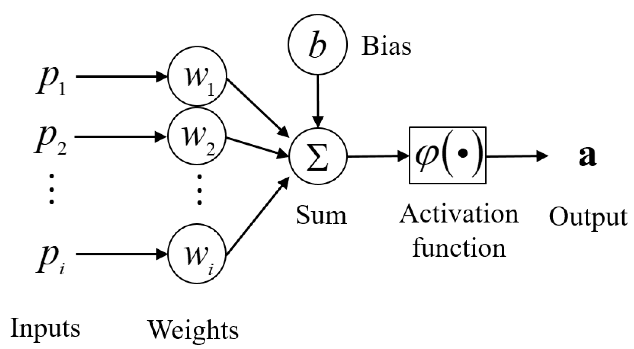
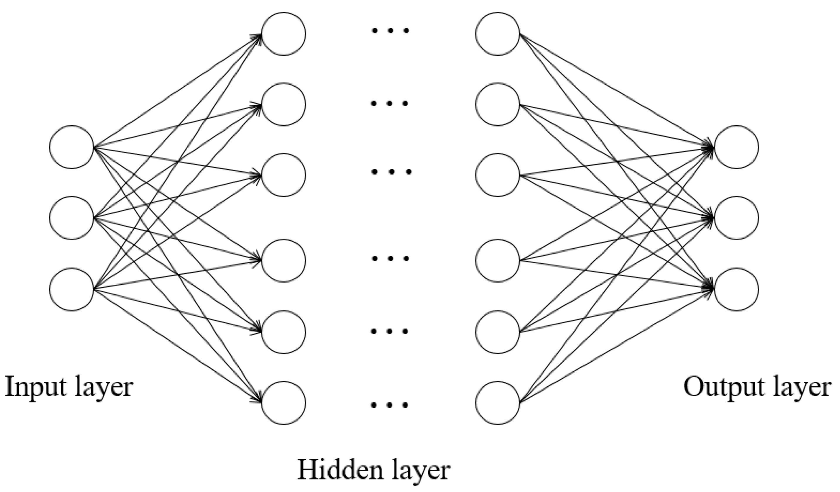
2.1. Neural Networks

Neural networks are a statistical data modeling tool made mostly of neurons, as shown in Figure 2. The parameter p denotes the parameters of an input datum and is multiplied by the weight and added to the bias. Next, the activation function is used to output a, and the expression can be written as:

$$\mathbf{a}=\phi (\mathbf{w}\mathbf{p}+\mathbf{b})$$

(1)

where w denotes weight, b denotes bias, and φ denotes activation function. Different activation functions are used when solving different types of problems. The sigmoid activation function is generally used in classification problems. For this function, output value approaches 1 or 0 when the input parameter values increase or decrease, respectively. By contrast, for regression problems, the rectified linear unit (ReLU) function is generally used. Positive input parameters are proportionally output as positive values, whereas negative values are output as zero, providing additional data features to regression problems. A neural network, which consists of input, hidden, and output layers, contains multiple neurons, as shown in Figure 3. The hidden and output layers are made of neurons, and different numbers of neurons and hidden layers create different neural networks models. By adding more neurons or more layers, neural network can represent a more complex nonlinear equation to approximate the actual functions of problems. The expression of neural network can be written as:

$${\mathbf{a}}^M={\phi }^M({\mathbf{w}}^M{\phi }^{M-1}({\mathbf{w}}^{M-1}\dots ({\phi }^1({\mathbf{w}}^1{\mathbf{p}}^0+{\mathbf{b}}^1))\dots +{\mathbf{b}}^{M-1})+{\mathbf{b}}^M)$$

(2)

where M is the number of layers, and the superscript indicate the layer number.

2.2. Backpropagation Algorithm

The backpropagation algorithm is a method for neural networks to update weights and bias values iteratively. According to the concept of sensitivity proposed by Rumelhart et al. [21], sensitivity can be used to express the strength of the effect that each neuron in each layer has on errors. Neural network weights and bias values can be updated according to the sensitivity as follows:

$${\mathbf{W}}_{k+1}^d={\mathbf{W}}_k^d-\alpha {\mathbf{s}}^d{\mathbf{a}}^{d-1}$$

(3)

$${\mathbf{b}}_{k+1}^d={\mathbf{b}}_k^d-\alpha {\mathbf{s}}^d$$

(4)

$$d=M-1, \dots , 2, 1$$

(5)

where W is weight matrix, b is bias vector, M is the number of layers, s is the sensitivity matrix, k is the iteration step, and α is the learning rate or iteration step size. The sensitivity between layers is as follows:

$${\mathbf{s}}^d=\dot{\phi }{ }^d({\mathbf{n}}^d){({\mathbf{W}}^{d+1})}^T{\mathbf{s}}^{d+1}$$

(6)

where $\dot{\phi }{ }^d({\mathbf{n}}^d)$ is the partial derivative of the activation function of the dth layer for the input value n. The backpropagation algorithm is named so because it calculates the sensitivity of each layer in a backward manner (i.e., from the next layer to the previous layer) [21,22]. The sensitivity in final layer in given by:

$${\mathbf{s}}^M=-2 {\dot{\phi }}^M({\mathbf{n}}^M)(\mathbf{t}-\mathbf{a})$$

(7)

where a is network’s output and t is the known actual output.

3. Water Tank Acoustic Field and Data Features

In the process of training a neural network, selecting appropriate data features can effectively reduce training costs, so it is very important to determine the data input form of the input layer. This study refers to the methods of Yangzhou et al. [15] and Shunsuke et al. [19] to process signal data. After comparing the accuracy of the two, the method by Yangzhou et al. with a lower error is used to select data features. The original approach is still not applicable to our cases due to the significant error caused by several area. Therefore, we introduced several corrections during the study including the min-max normalization, floating-point number processing and optimization-based loss functions to further improve the quality of the data and increase the accuracy of the prediction results.

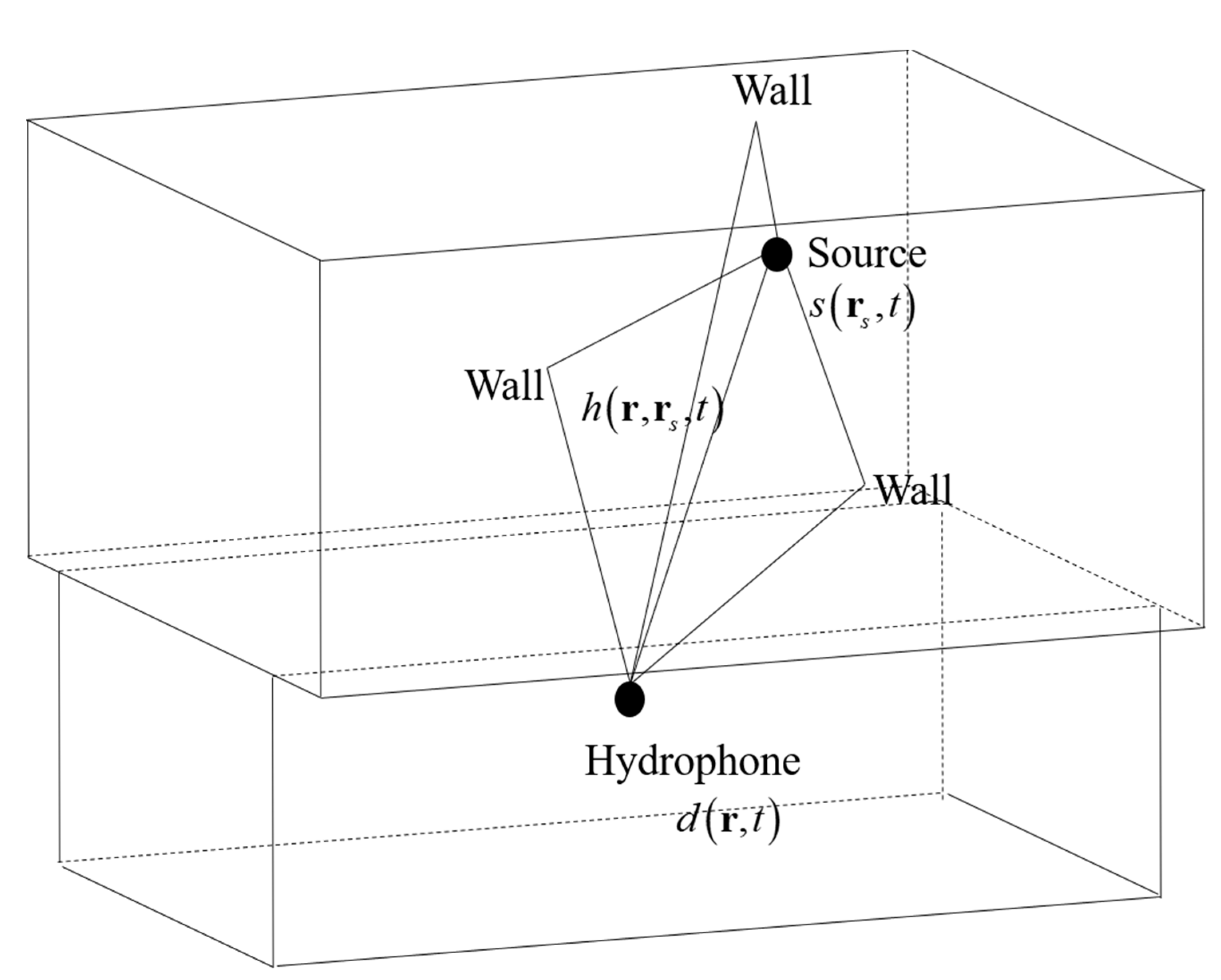
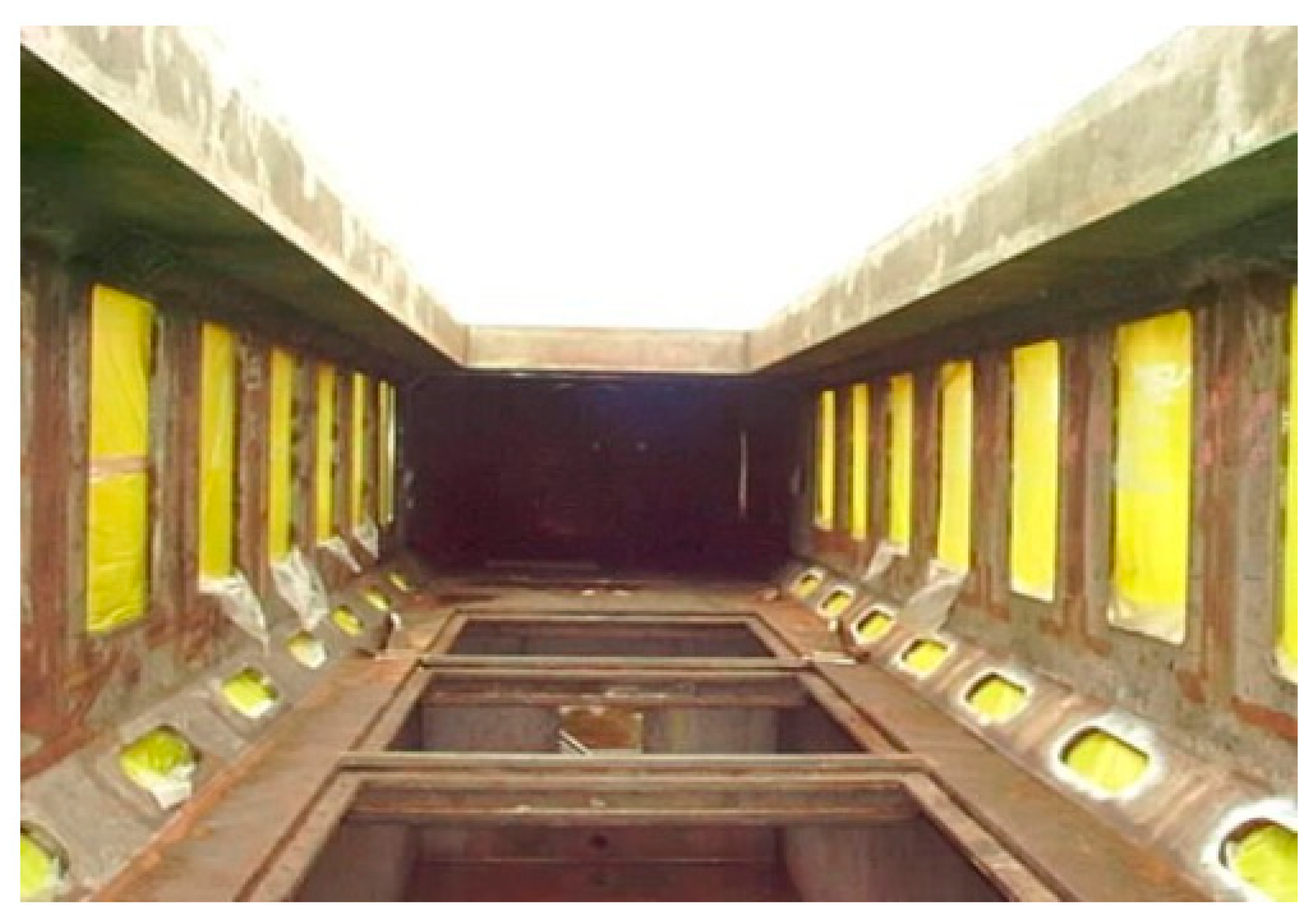
3.1. Setting of the Water Tank Acoustic Field

In this study, neural networks were used to locate acoustic sources inside a cavitation tank. Based on the descriptions of signal transmissions in cavitation tanks provided by Park et al. [15], the present study adopted the paths displayed in Figure 4 as signal transmission paths and the equation for time-domain signal z(r, t) received by a microphone is as follows:

$$z\left(r,t\right)=s\left(r_s,t\right)\times h\left(r,r_s,t\right)+g\left(r,t\right)$$

(8)

where r and r_s are the vectors of the hydrophone and acoustic source location, respectively, t is the time, s is the acoustic time-domain signal from the source, h is the convolution impulse response function, and g is the background noise in the environment. By implementing the Fourier transform, Equation (8) can be written as a frequency-domain equation as follows:

$$Z\left(r,\omega \right)=S\left(r_s,\omega \right)\times H\left(r,r_s,\omega \right)+G\left(r,\omega \right)$$

(9)

where ω is frequency. The capitalized symbols in Equation (9) correspond to the lowercase symbols in Equation (8). When describing microphone arrays, Equation (9) can be expressed in the form of a matrix as follows:

$$Z\left(r,\omega \right)=S\left(r_s,\omega \right)\times H\left(r,r_s,\omega \right)+G\left(r,\omega \right)$$

(10)

The convolution impulse response function matrix is equivalent to the black box of a water tank environment and sound transmission in that it can be obtained only after multiple experimental measurements or numerical simulations have been performed. Park et al. [8] presented this matrix by using the following simple conversion formula:

$$H\left(r,r_s,\omega \right)={\displaystyle \sum _{i=1}^{\infty }{A}_i}\left(r,r_s,\omega \right)e^{i{\psi }_i\left(r,r_s,\omega \right)}$$

(11)

The summation symbol denotes the sum of the superpositions of direct waves and all reflected waves in a water tank, and A and ψ are the intensity and phase angle of the signal when the signal reaches the microphone, respectively. In the study of Park et al. [8], only the effects of direct waves were considered.

$$H\left(r,r_s,\omega \right)=\frac{1}{\left|r-r_s\right|}{e}^{i\omega \frac{\left|r-r_s\right|}{c_0}}$$

(12)

In Equation (12), c₀ is the wave speed. The objectives of the present study were to use neural networks to construct an impulse response function similar to Equation (9) and to use the finite-volume method software ANSYS Fluent 2022 R1 to generate the data required for training neural networks. The finite volume method was used as an alternative to the method expressed in Equation (12), in which only the conversion formula of direct waves is considered.

3.2. Data Feature Extraction

When training neural networks, determining the data input methods for the input layer is crucial because appropriate data feature selection can effectively reduce training costs.

The normalized sample covariance matrix method of Yangzhou et al. [15], which is commonly used in acoustic imaginary partial analysis, was selected as the neural network input method in this study. The sample covariance matrix comprises time-domain signals received from K microphones at n time points. The time-domain signals received from single microphone can be express as follows:

$$S_i={\left[S_{i1} S_{i2} \cdots S_{ij}\right]}^{\mathrm{T}},i=1,2,\dots ,K,j=1,2,\dots ,n$$

(13)

where i denotes ith microphone and denotes jth time points. In this study, the FFT was implemented on frequency signals (numbered 1~c by frequency) to obtain the following equation:

$$F_i={\left[F_{i1} F_{i2} \cdots F_{im}\right]}^{\mathrm{T}},i=1,2,\dots ,K,m=1,2,\dots ,c$$

(14)

where m denotes mth frequency. The vector composed of all receivers is defined as follows:

$$B={\left[F_1 F_2 \cdots F_i\right]}^{\mathrm{T}},i=1,2,\dots ,K$$

(15)

Moreover, the normalized sample covariance matrix is calculated as follows:

$$C_{q\times q}=B{B}^H$$

(16)

where the superscript H is the complex conjugate transpose, and q denotes the size of the normalized sample covariance matrix. This matrix was converted into a one-dimensional, real-number vector that could serve as a suitable neural network input. In this study, the aforementioned matrix was split into vectors that comprised real and imaginary parts and were 2q² in size. The expression can be written as:

$$D={\left[\mathrm{Re}\left(C_{11}\right) \cdots \mathrm{Re}\left(C_{qq}\right) \mathrm{Im}\left(C_{11}\right) \cdots \mathrm{Im}\left(C_{qq}\right)\right]}^{\mathrm{T}}$$

(17)

where Re and Im denote the real parts and imaginary parts, respectively. These parts were used as data feature inputs in neural networks. This study also referred to the method of Shunsuke et al. [19] and use the absolute value of frequency as the data feature form. The single-receiver-frequency data vector is expressed as follows:

$$R_{im}=\sqrt{\mathrm{Re}{\left(F_{im}\right)}^2+\mathrm{Im}{\left(F_{im}\right)}^2},i=1,2,\dots ,K, m=1,2,\dots ,c$$

(18)

$$R_i={\left[R_{i1} R_{i2} \cdots R_{im}\right]}^{\mathrm{T}},i=1,2,\dots ,K, m=1,2,\dots ,c$$

(19)

Moreover, the vector comprising all receivers is represented as follows:

$$B={\left[R_1 R_2 \cdots R_i\right]}^{\mathrm{T}}$$

(20)

The initial architecture of the neural network comprised eight hidden layers that had 100 neurons each. A rectified linear function was used as the activation function of the hidden layer, and a linear function was used as the activation function of the output layer. In the initial setup, the mean squared error (MSE) was selected as the target loss function for network learning. The MSE is defined as follows:

$$L_{MSE}=\frac{1}{N}{\displaystyle \sum _{i=1}^N{\left(T_i-Y_i\right)}^2}$$

(21)

where T_i and Y_i are the predicted and actual values, respectively, and N is number of data. The results of using mean absolute error (MAE) instead of MSE for the target loss functions are presented in Section 4.5. The MAE is defined as follows:

$$L_{MAE}=\frac{1}{N}{\displaystyle \sum _{i=1}^N\left|T_i-Y_i\right|}$$

(22)

Regardless of whether MSE or MAE is used, the objective is to minimize losses and find the optimum solution. The main difference is that MSE will amplify the error in order to the achieve larger gradient and rapid descending of error. This will easily lead to faster and unstable convergence when the input data consist of large amount of error. Therefore, we will compare the influence of two lose functions in Section 4.5 and Section 5.2 and find which is more suitable for the localization problem. This study used the backpropagation algorithm to update network weights and bias values, and the Adam optimizer [23] was employed to update and optimize the learning rate and reduce the training time. The number of time steps was set as 10⁵, and training data were input for training, which was performed on an Intel Core i5-4460 CPU with a 3.20-GHz processor, 32 GB of memory, and an NVIDIA GeForece GTX 750 graphics card. The neural network is implemented in Python 3.7 and TensorFlow 2.5.

4. Numerical Simulation on the Simple Rectangular Cuboid Acoustic Field Model

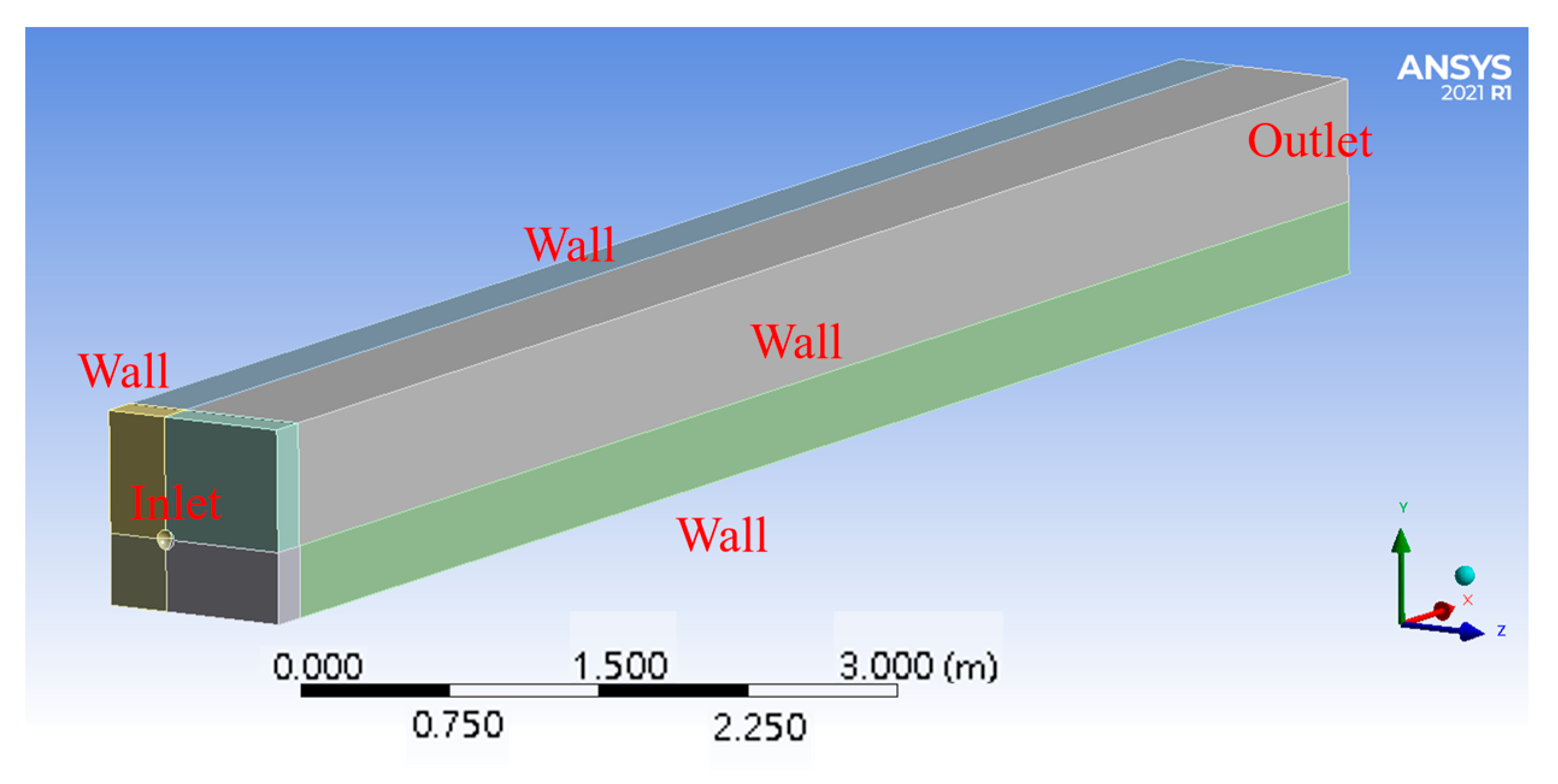
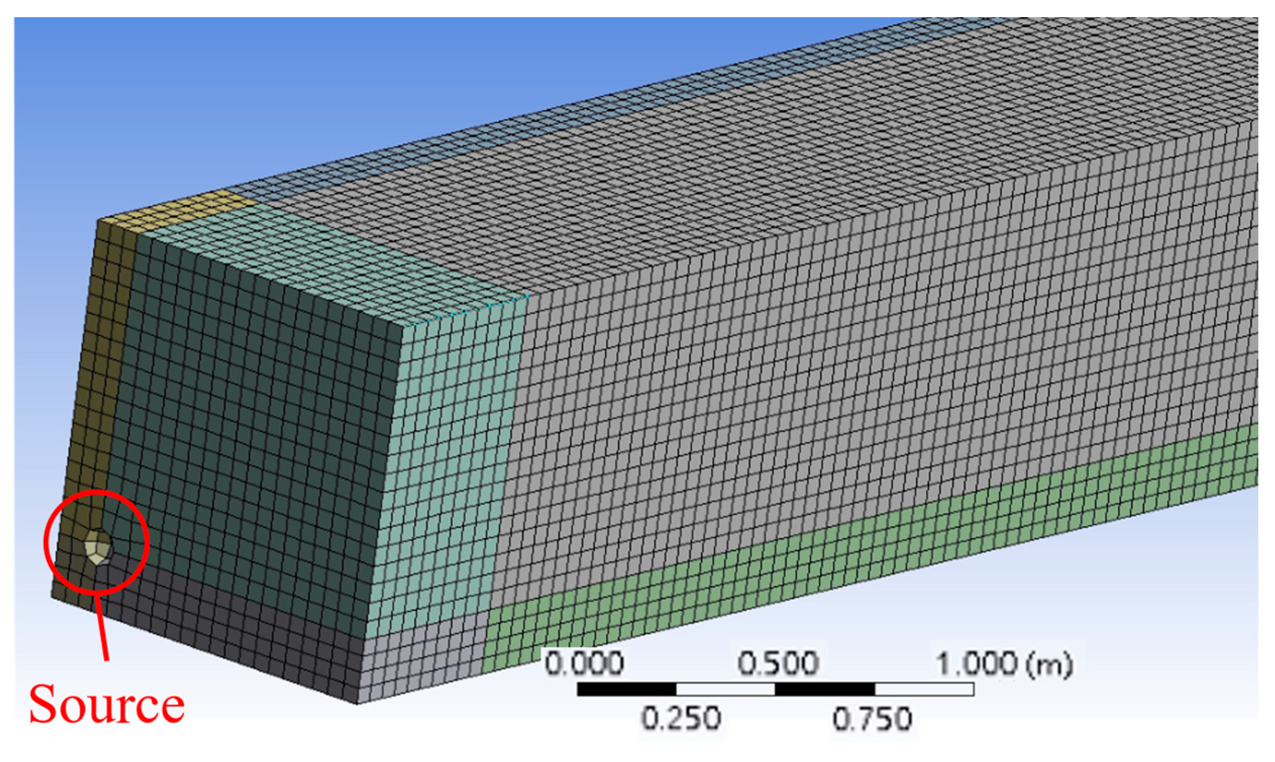
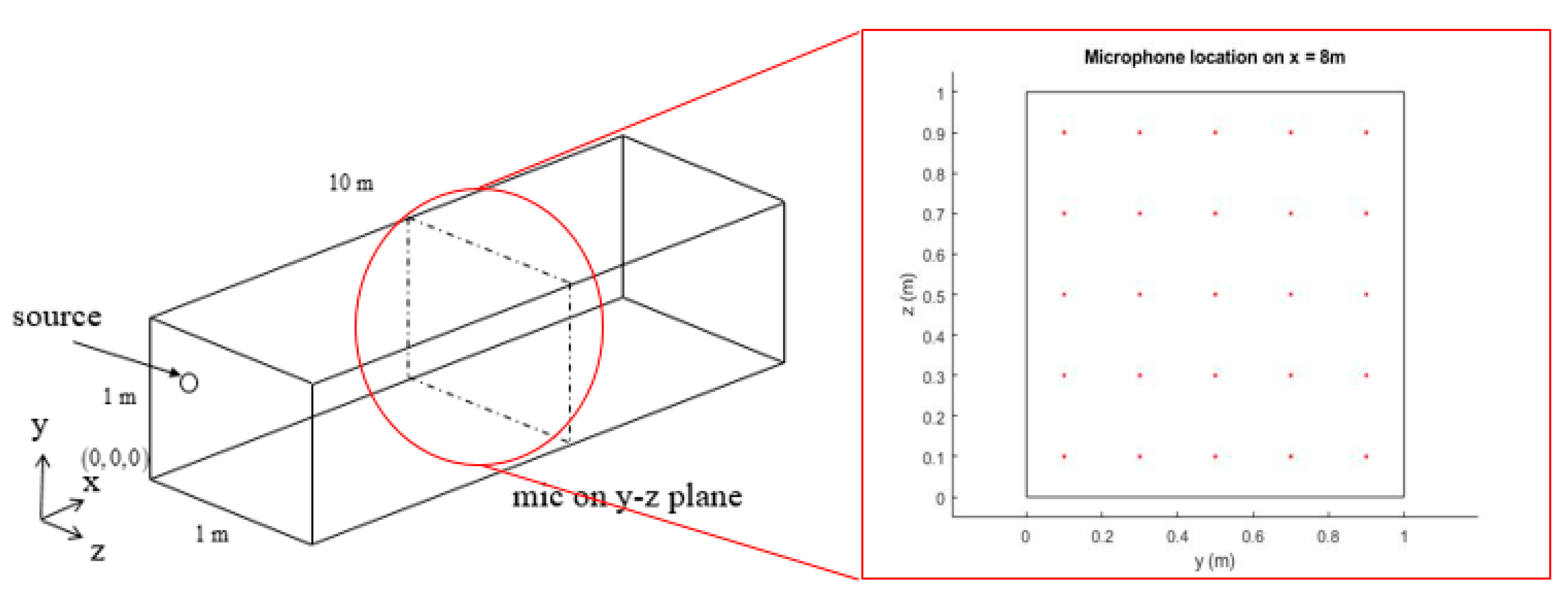
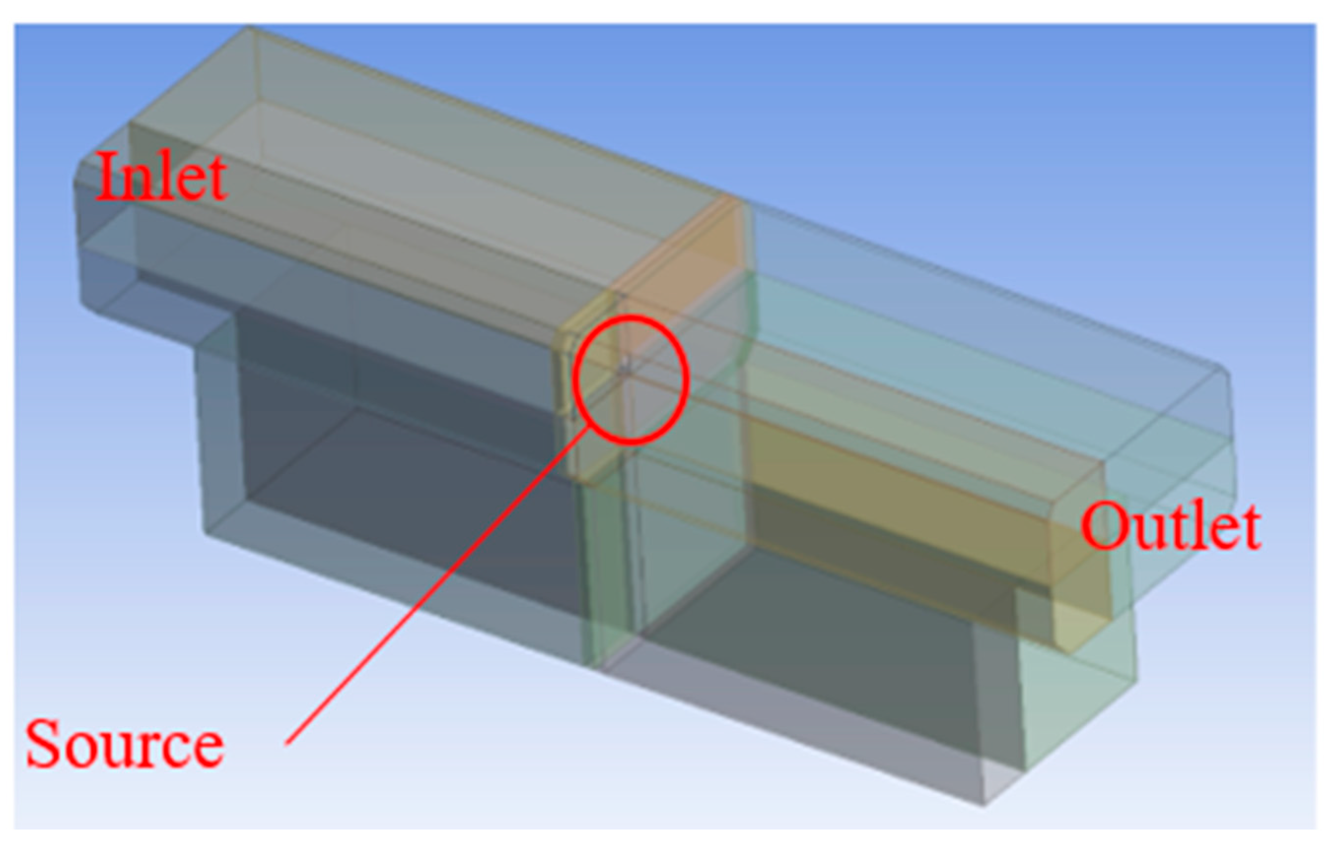
4.1. Numerical Setup

To test the effects of neural network input data on the training results, a simple rectangular cuboid acoustic field model was constructed. This model had a length, width, and height of 10, 1, and 1 m, respectively (Figure 5). In this study, the length of the square grid [24] was set as 0.05 m (Figure 6). Liquid water with a sound speed of 1482.1 m/s and a density of 998.2 kg/m³ was selected as the medium. As the initiation research of this difficult subject, we start with simple assumptions of ignoring temperature change and any flow influence such as cavitation, for the numerical experiments. A tiny vibration sphere [25] with the following vibration equation was set as the acoustic source:

$$P=77\cos \left(2\pi \cdot 295.55\cdot t\right)+23\sin \left(2\pi \cdot 281.86\cdot t\right)$$

(23)

The effects of water flow and background noise in the tank were not considered, and the microphone array was set symmetrically on a plane parallel to the inflow section, as shown in Figure 7. In this study, the shear stress transport k–ω model was used, the effects of gravity were ignored, the time step length was set as 0.00001 s, and the number of time steps was set as 20,000 to allow the wave propagation model to reflect completely. The data segments from 0.1 to 0.2 s were taken and processed. This procedure produced a total of 2660 pieces of acoustic source data for different positions, 2390, 265, and 5 of which were used for training, verification, and testing, respectively.

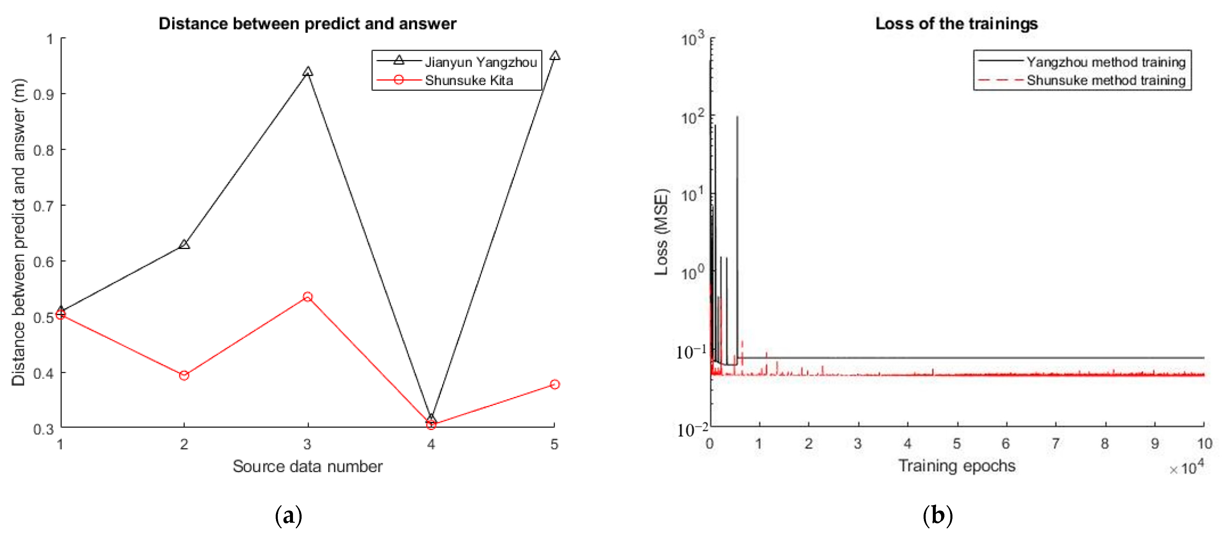
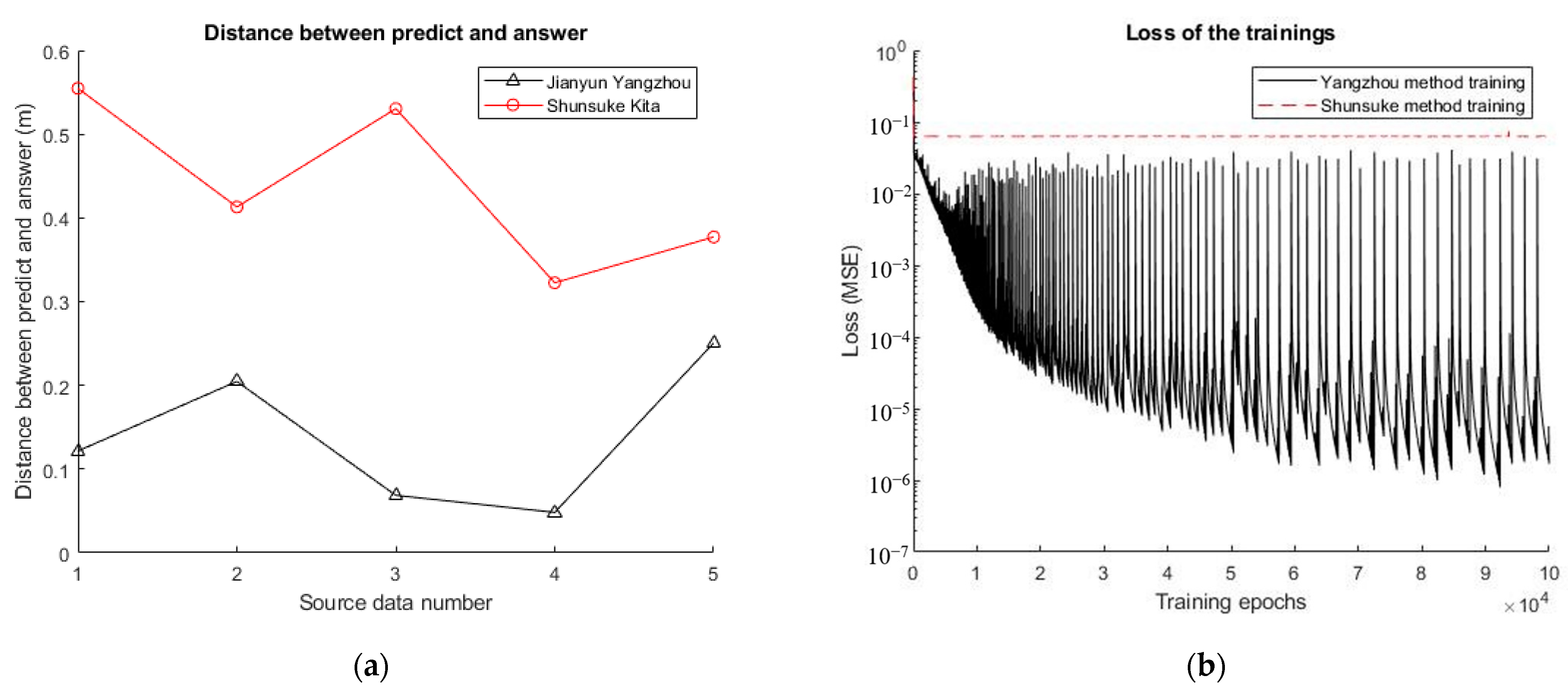
4.2. Comparison between the Yangzhou’s Method and Shunsuke’s Method Prior to Min–Max Normalization

This section describes the data feature selection methods of Yangzhou et al. [15] and Shunsuke et al. [19]. The performance of these methods when using MSE as the loss function of a neural network is compared. Figure 8a shows the distance errors between the prediction results and actual acoustic source locations. Figure 8b depicts the loss function convergence results. Figure 8c,d display the training data loss epochs. The prediction results indicated that both methods were not ideal for solving the problems examined in this study. The distance errors between the actual and predicted acoustic source locations were higher than 0.3 m. The distance error for Yangzhou’s method was as high as 0.9 m, which approached the maximum width of the rectangular cuboid model. In addition, because ReLU was used as the activation function, the negative inputs automatically became 0 when Yangzhou’s method was used, which resulted in some data features being lost. The average minimum loss function value of Yangzhou and Shunsuke was 0.316 and 0.045 respectively, which suggested that for the training data, the training prediction results had a distance error of 0.566 m and 0.212 m. The reasons for the errors might be that the training time was insufficient and that small parameter features were ignored.

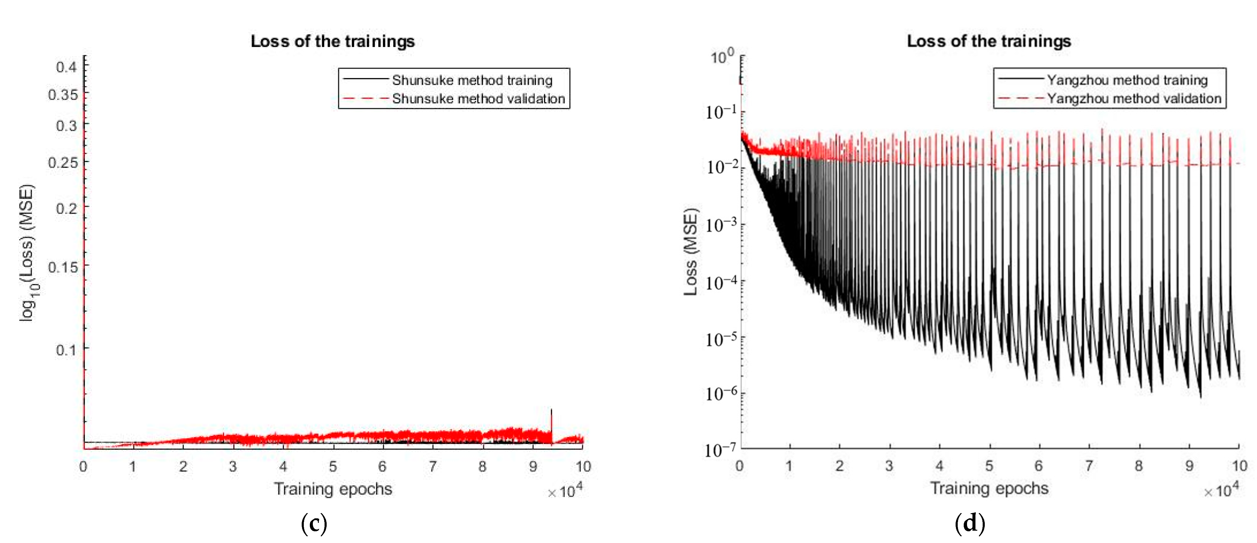
4.3. Comparison between Yangzhou’s Method and Shunsuke ‘s Method after Min–Max Normalization

Next, this study examined how min–max normalization limited the parameter range of different data between 0 and 1 under the same frequency and compared the effects of such normalization on Yangzhou’s method and Shunsuke’s method. By using the min-max normalization, we limited the influence of amplitude with different frequencies. This will avoid the overfitting of the prediction result to certain frequency because it has larger amplitude. It can also ensure the information of small-amplitude data been captured by the data base. The prediction results obtained with these methods after min–max normalization are shown in Figure 9a. Figure 9b depicts the loss function convergence results. Figure 9c,d display the training data loss epochs.

The predictions obtained using Yangzhou’s method after min–max normalization and the actual acoustic source locations differed by less than 0.3 m on average and were as close as within 0.04 m. Overall, predictions errors that occurred when using Shunsuke’s method were greater than those that occurred when using the Yangzhou’s method after min–max normalization, which indicated that the method of Yangzhou et al. was more suitable for this study. Nevertheless, the predictions obtained using Yangzhou’s method produced an average distance error of 0.15 m. In this study, an improved method based on Yangzhou’s method was proposed to further reduce the errors.

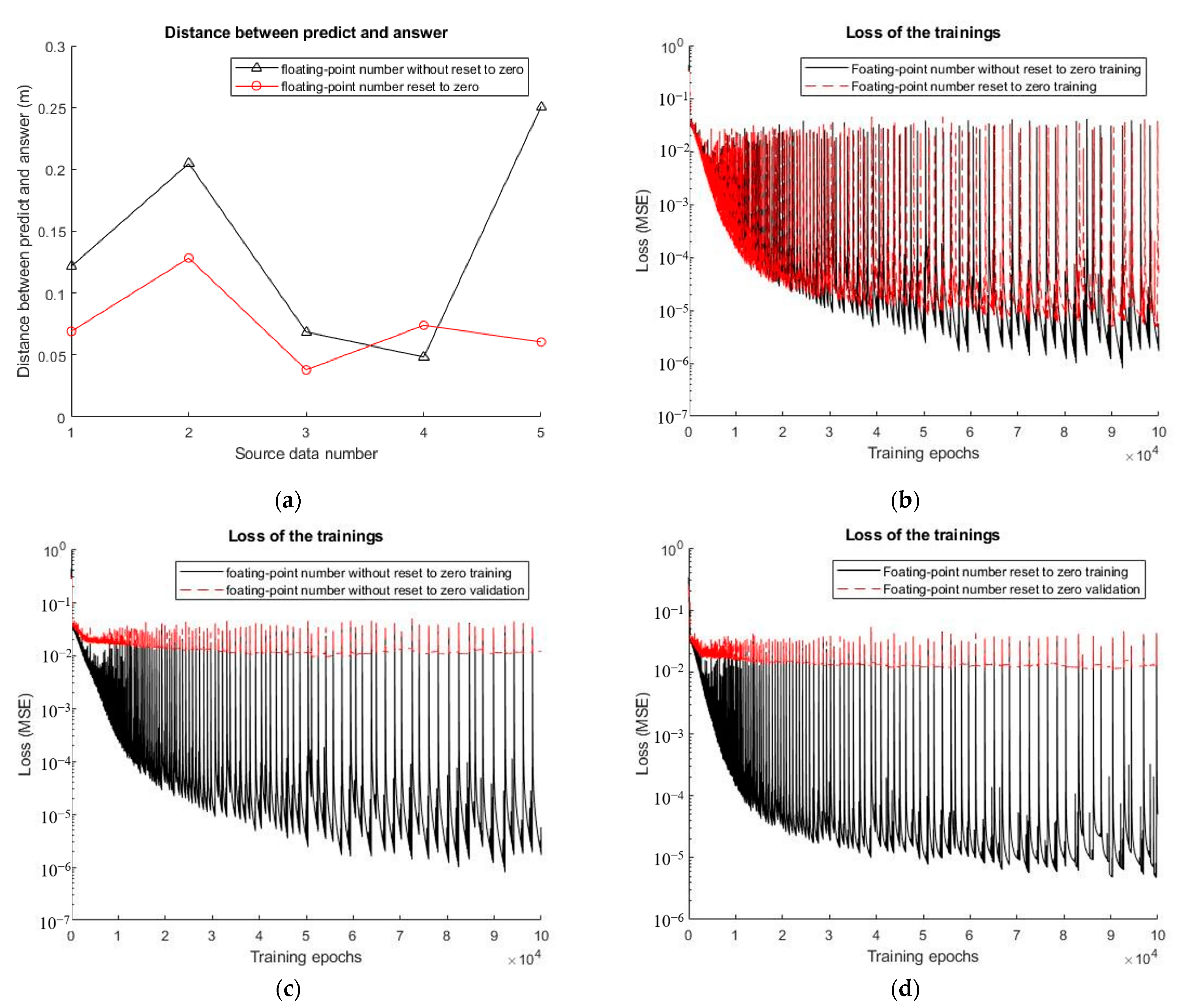
4.4. Optimizing the Yangzhou’s Method through Floating-Point Number Preprocessing

A review of the method of Yangzhou et al. and its equations revealed that after the vectors comprising real and imaginary parts are multiplied by their conjugate transpose vectors, the imaginary part along the diagonal of the matrix shows a value of 0. In actual practice, because of the influence of floating-point numbers, the value of the imaginary part is an extremely small random number, resulting in its random number feature being magnified in min–max normalization. This in turn caused the training data to contain random feature parameters that are not logically related to the solutions. Therefore, in this study the extremely small values caused by floating-point numbers were set to 0, so that the data less than 10⁻⁶ before normalization were reset as 0, whereas the remaining values were left unchanged. Normalization was performed only after the aforementioned preprocessing was implemented. Figure 10a shows the distance errors (i.e., the differences between the prediction results and actual acoustic source locations) obtained when normalization was performed after data preprocessing. Figure 10b depicts the loss function convergence results. Figure 10c,d display the training data loss epochs obtained before and after floating-point number preprocessing. After the small values caused by floating-point numbers were reset to 0, the method of Yangzhou et al. was improved, which resulted in an average error of less than 0.1 m in the predictions of acoustic source locations.

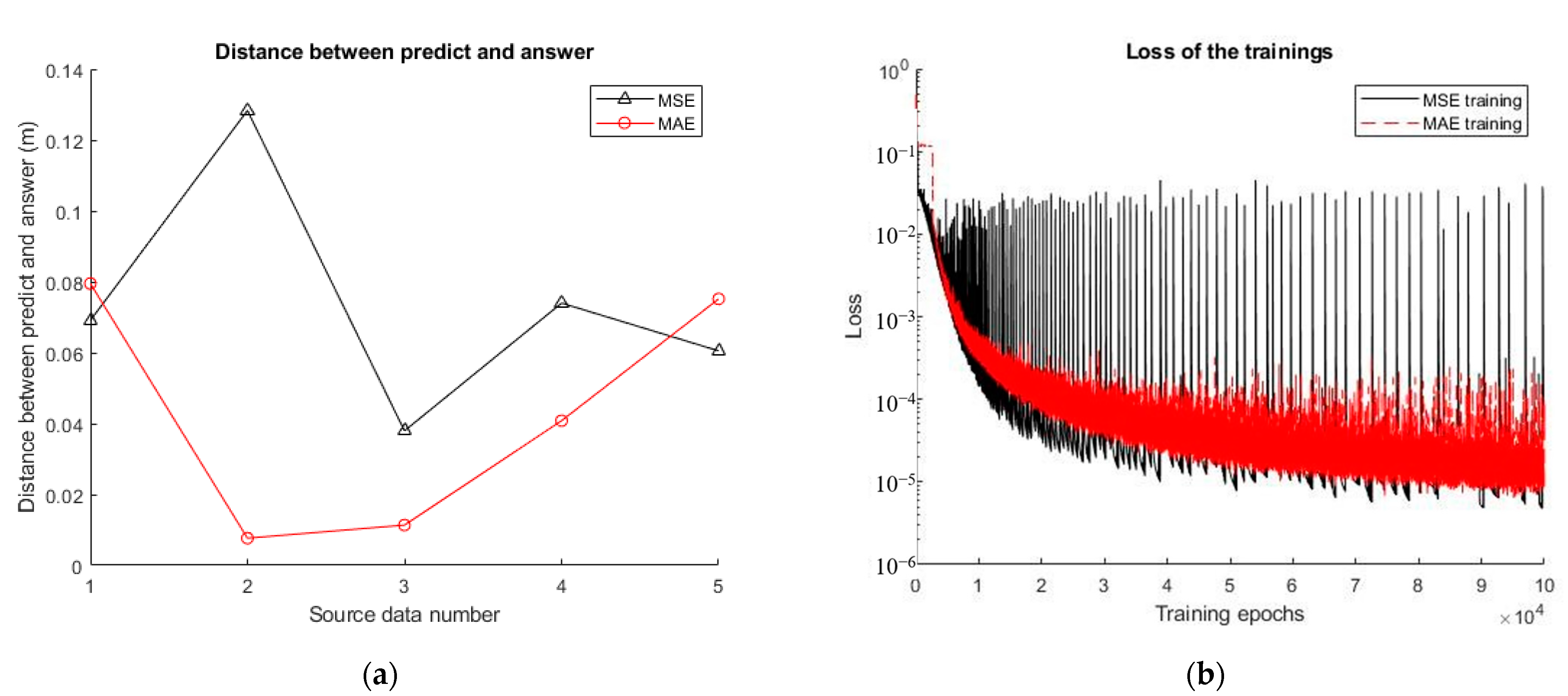
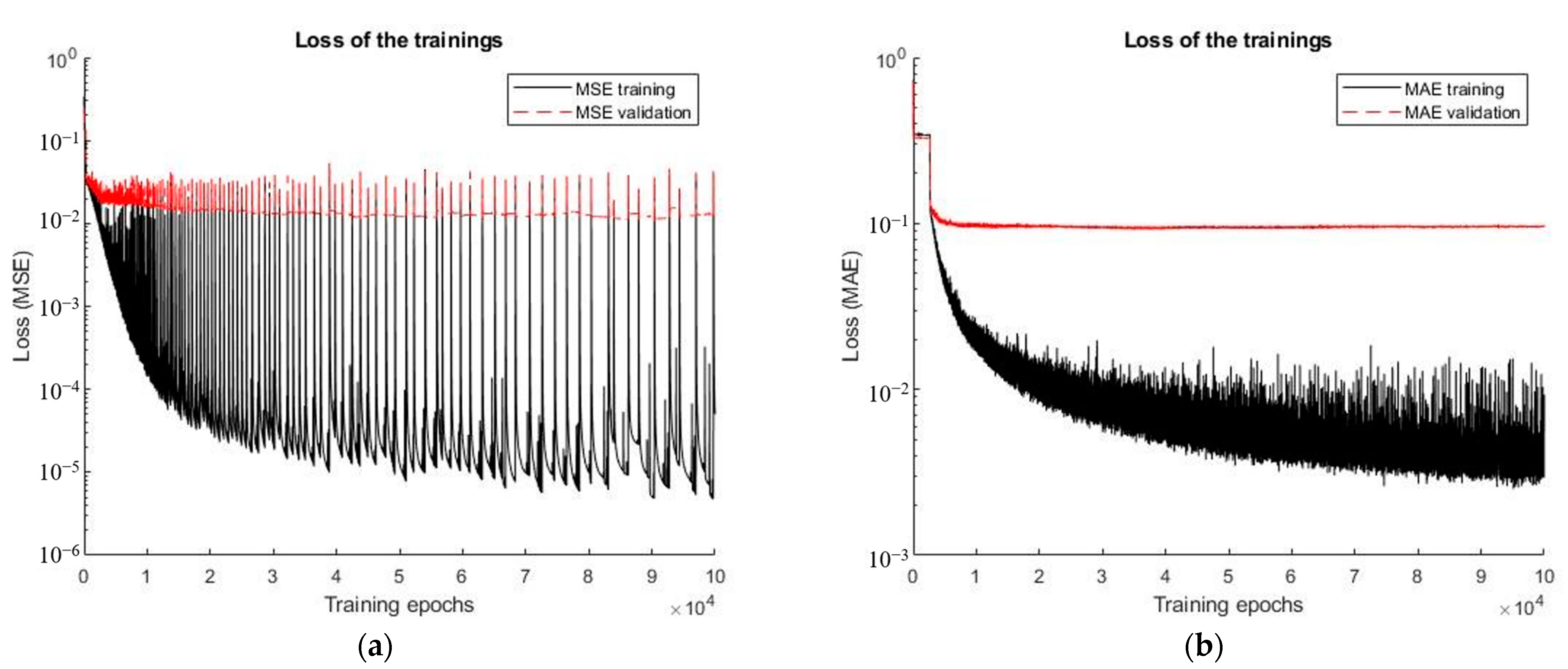
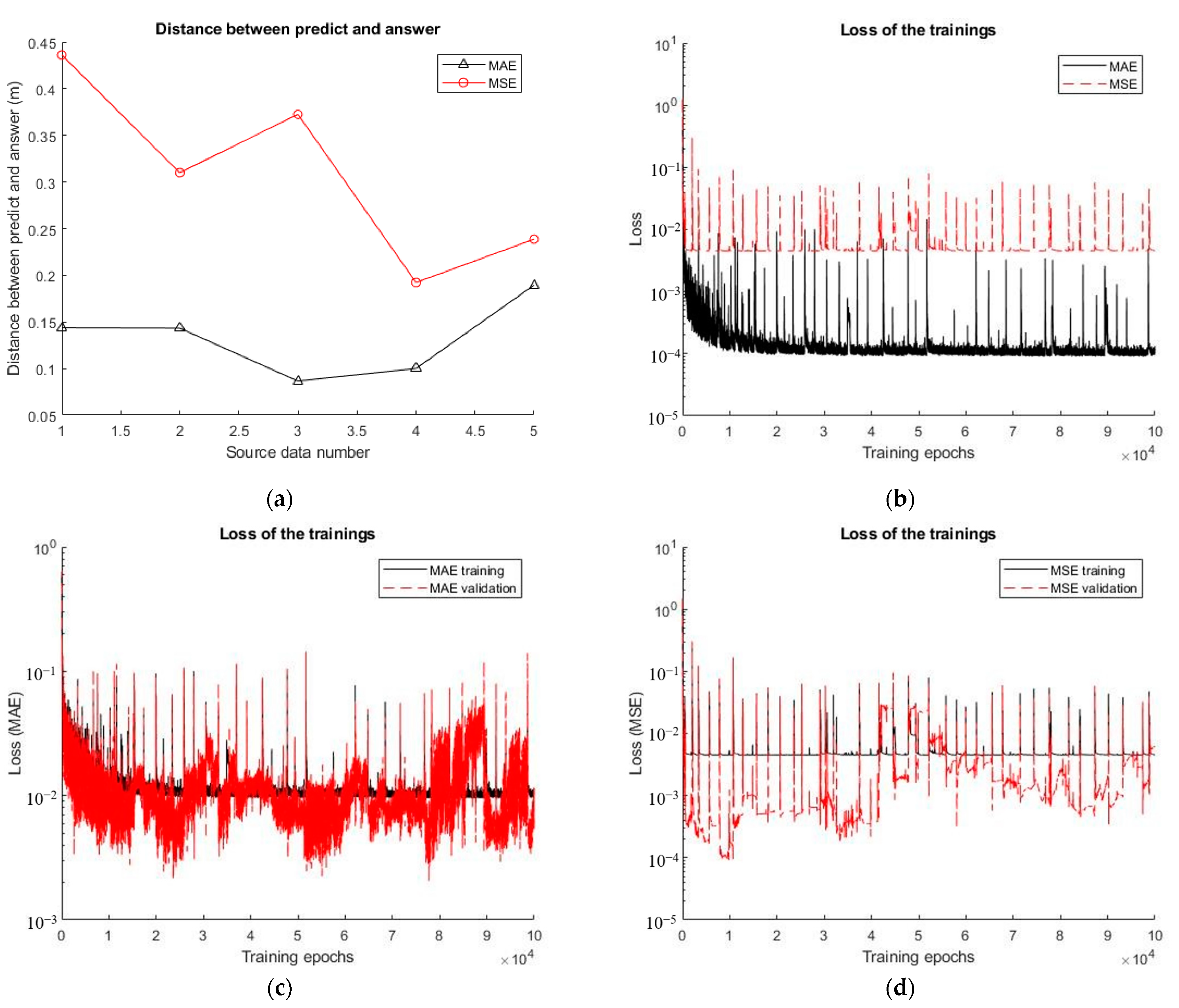
4.5. Effects of the MSE and MAE as Loss Functions on Training

Shunsuke et al. and Yangzhou et al. did not examine the effects of the loss function on the prediction results. Thus, this study compared the prediction results obtained using neural network models that were trained using either MSE or MAE as the loss function after min–maximum normalization was performed on the data. The errors between the predicted results and the actual acoustic source locations are shown in Figure 11a. To ensure that the results using the MAE and the MSE could be compared on the same scale, the losses generated when the MAE was used had to be squared before comparisons were conducted. The loss function convergence results obtained with the MSE and MAE are displayed in Figure 11b. Moreover, the verification training epochs obtained when using the MSE and MAE are displayed in Figure 12a,b, respectively. Figure 11a indicates that on average, the neural network model trained using the MAE as the loss function produced more accurate prediction results than did that trained using the MSE as the loss function. When using the MAE as the loss function, the minimum difference between the predicted and actual acoustic source locations was 0.008 m. However, when using the MSE as the loss function, the minimum difference between the predicted and actual acoustic source locations was 0.038 m. According to the training process displayed in Figure 11b, although the neural network model trained using the MAE had a higher minimum loss than that trained using the MSE, the drops in losses during the training process were more stable for the model trained using the MAE than for that trained using the MSE. On the basis of the aforementioned results, the MAE was selected as the loss function in this study because it produced more accurate prediction results and had more steady drops in losses during the training process than did the MSE.

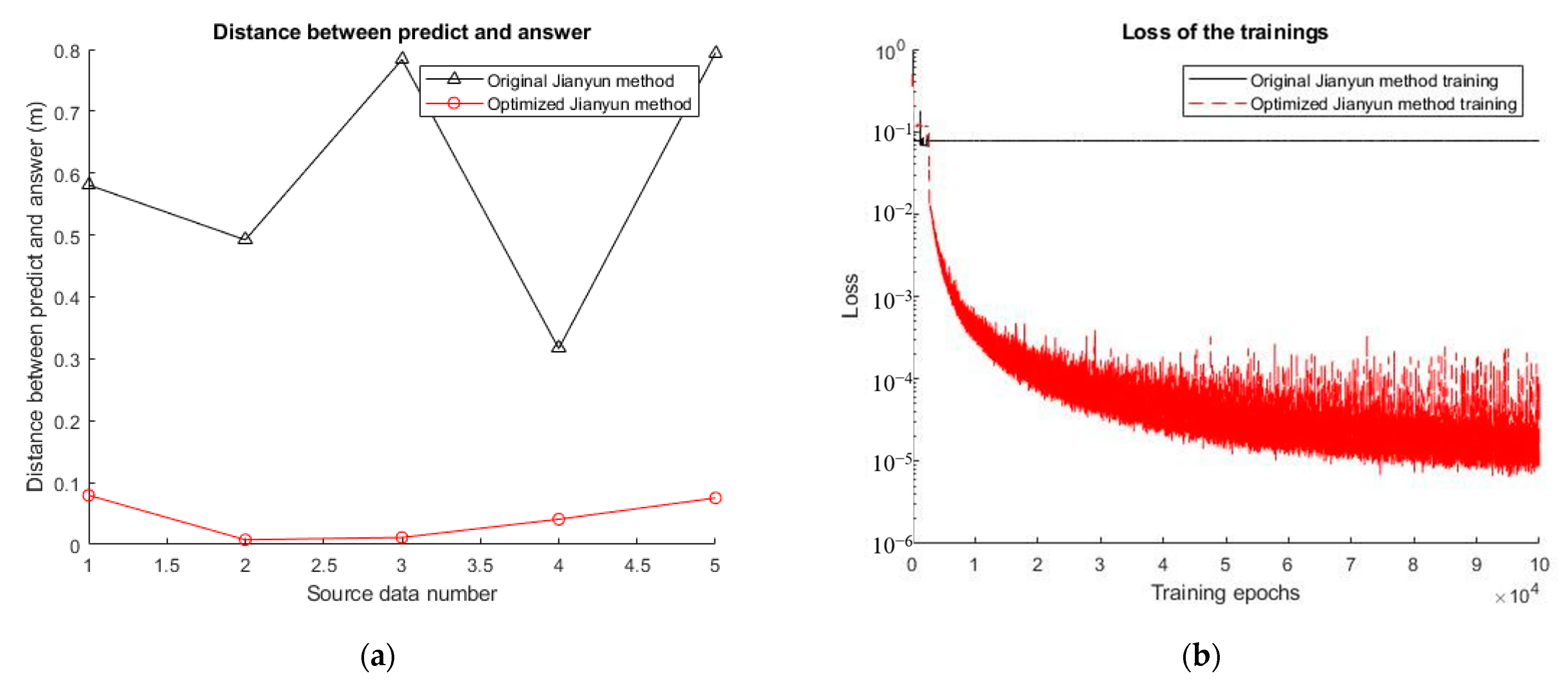
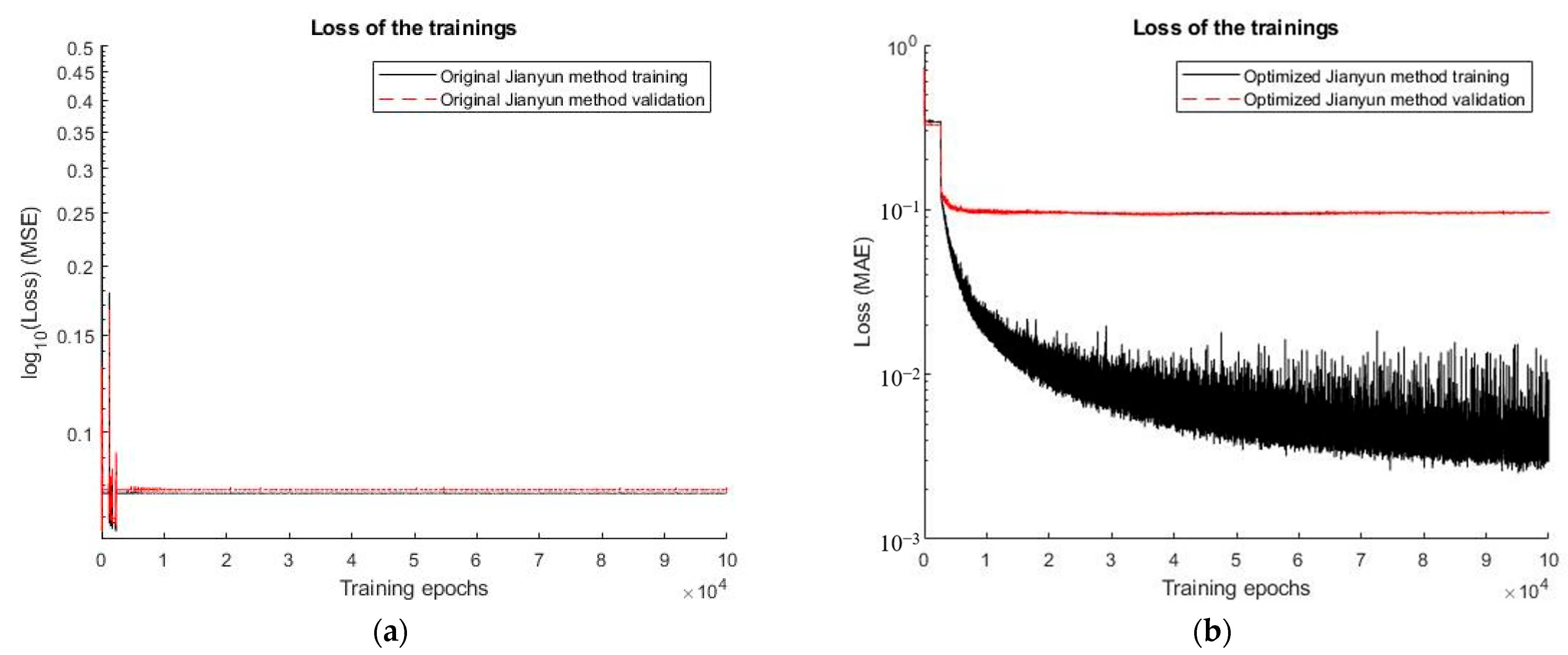
4.6. Comparison of the Yangzhou’s Method before and after Optimization

In contrast to tanh function which used by Yangzhou et al., ReLU function is more popular activation function in the neural network framework. The advantage is that it avoid the vanishing gradient problem caused by other activation functions such as sigmoid and tanh. The results obtained by Yangzhou et al. by using tanh activation functions were compared with those obtained using the neural network model (with unregularized data) trained using the MAE (in which the ReLU activation function was used) in this study. The prediction results and training epochs obtained when using tanh activation functions and the ReLU activation function are shown in Figure 13a,b, respectively. Moreover, the verification training epochs obtained using these functions are displayed in Figure 14a,b, respectively. Figure 13a indicates that Yangzhou’s method produced more accurate results after optimization than before optimization.

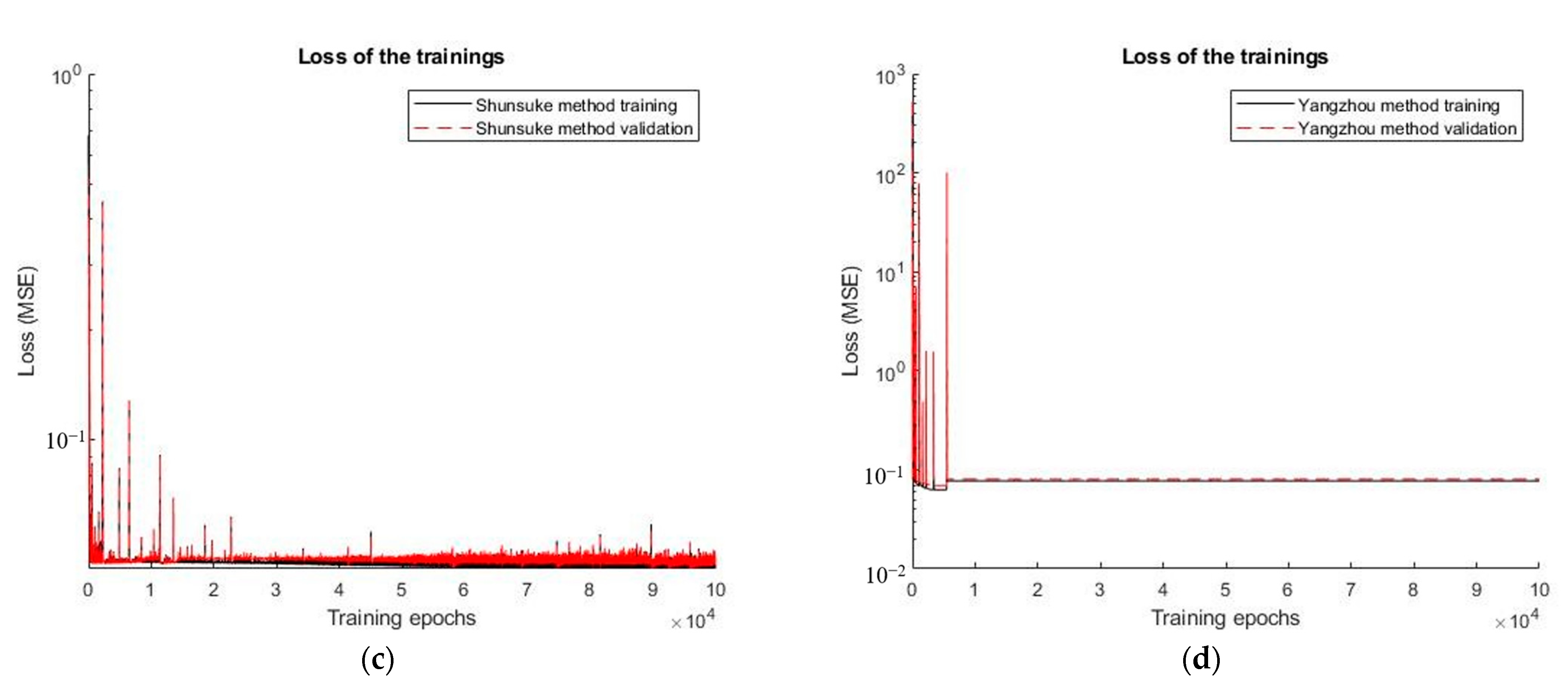
5. Numerical Simulation on a Large Cavitation Tank Acoustic Field Model

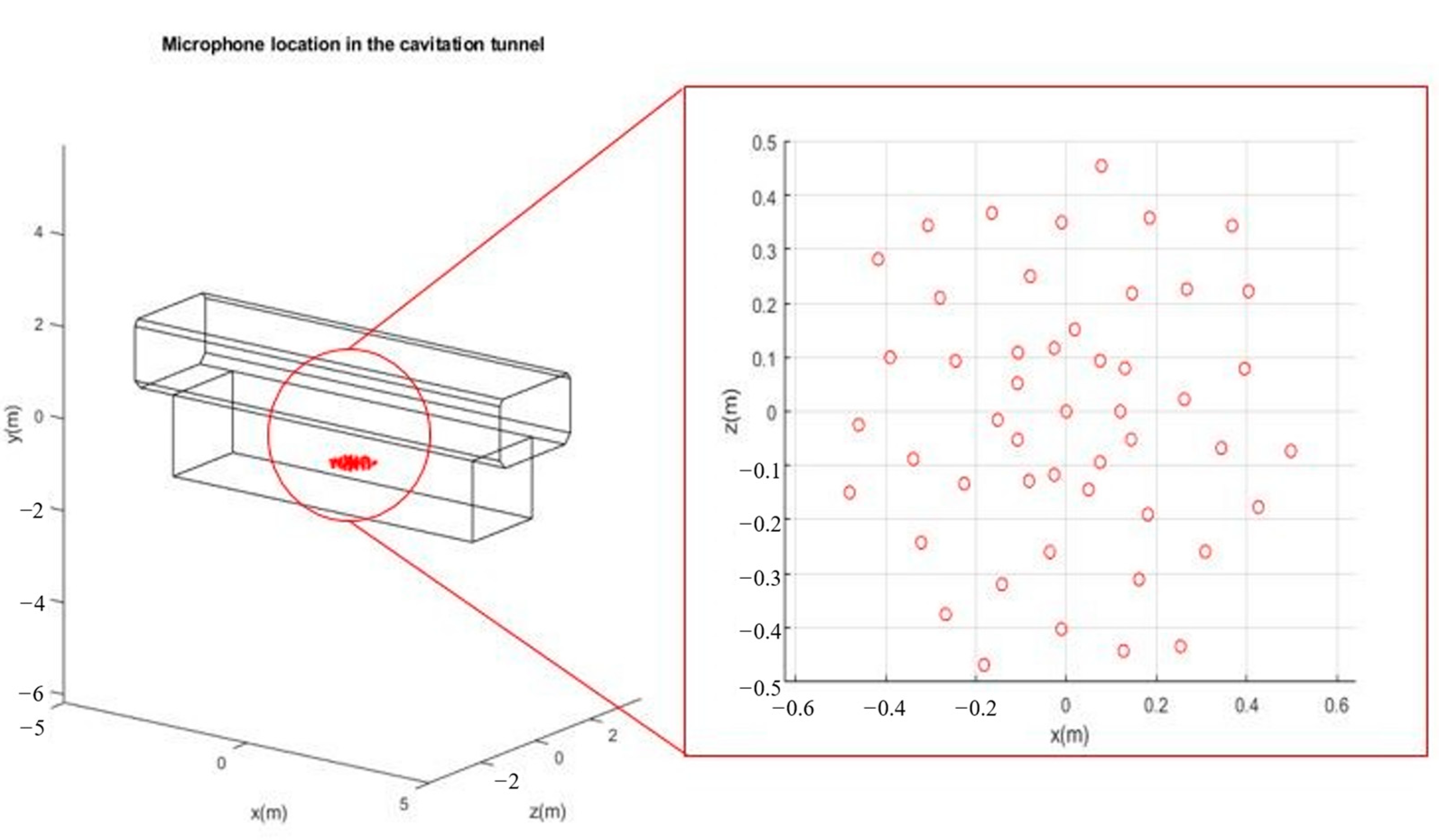
5.1. Numerical Setup

The geometric model of the large cavitation tank used in this study was based on the test section and anechoic chamber of the large cavitation tank at National Taiwan Ocean University, which is shown in Figure 15. As depicted in Figure 16, the test section of this tank is an octagonal column-like space that has a length, width, and height of approximately 10, 2.6, and 1.5 m, respectively. The anechoic chamber of the tank is a rectangular cuboid space with a length, width, and height of approximately 8.2, 2.2, and 1.77 m, respectively. The method for constructing the acoustic source locations was identical to that for constructing the acoustic source locations in the simple rectangular cuboid model. This model is represented by a sphere with a vibrating surface, and the pressure change at this surface can be expressed as follows:

$$P=77\cos \left(2\pi \cdot 397.89\cdot t\right)+23\sin \left(2\pi \cdot 413.8\cdot t\right)$$

(24)

The grid size was set as 0.05 m, and the water inlet and outlet of the test section were set as the pressure outflow boundaries. The other outer boundaries of the model were all full reflection boundaries. The design of the microphone array was based on that of James [26]. A total of 50 microphones were arranged in a spiral (Figure 17) and placed in the center of the anechoic chamber. The microphones were located 0.748 m from the bottom of the chamber. The calculation time step was set as approximately 0.00001 s, and the number of calculation time steps was set as 20,000. Next, the data at 0.1–0.2 s, which had relatively complete signal reflections, were used as the main data. The total number of data was 115, and the y values of all acoustic source locations were 0.75 m. A total of 100 pieces of data were used for training, ten pieces were used for verification, and the remaining five pieces of data were used for testing. The initial neural network architecture was identical to that mentioned in Section 3.2.

5.2. Effects of the MSE and MAE as Loss Functions on Training

To verify whether the effects of loss function selection on the prediction results varied between different models, the MAE and MSE were used as loss functions in the testing. The training epochs obtained when using these functions are shown in Figure 18. For the actual acoustic source locations (0.2, 0.75, 0.5) and (0.3, 0.75, −0.5), the locations predicted by the neural network trained using the MAE as the loss function were (−0.214, 0.750, 0.362) and (0.028, 0.750, −0.351), respectively, and the locations predicted by the neural network trained using the MSE were (0.150, 0.750, 0.366) and (0.441, 0.750, −0.525), respectively. The prediction results obtained using the two neural networks have larger errors than the results obtained in cuboid model test, with the average error reaching 0.3 m and 0.13 m, respectively. However, the neural network trained using the MAE had considerably lower losses than that trained using the MSE (Figure 18); thus, the neural network trained using the MAE was more suitable for this study.

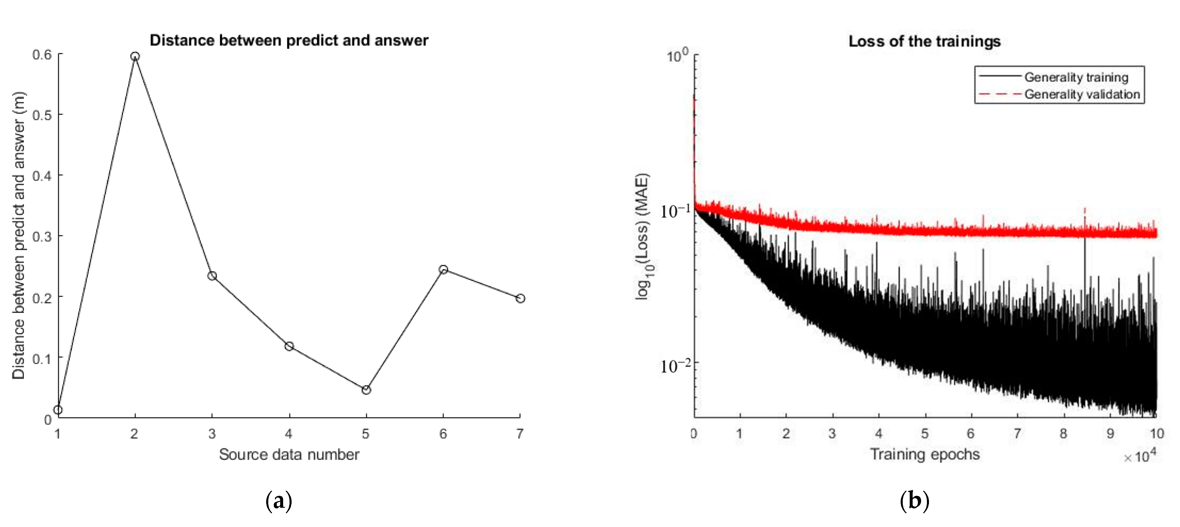
5.3. Universal Applicability Test

The universal applicability of the adopted neural networks was tested using the optimal data processing method. A total of 2655 pieces of data from the acoustic source database of the simple rectangular cuboid model and 110 pieces of data from the acoustic source database of the large cavitation tank model were selected as the neural network training data, with one-tenth of the training data being set aside as the verification data. The remaining data were used as the testing data. The final prediction results, prediction errors, and training epochs are presented in

Table 1. Prediction results obtained by combining the data of the rectangular cuboid model and large cavitation tank model.

Number	Model	Acoustic Source Location
		Actual	Predicted
1	Cavitation tank	(0.2, 0.75, 0.5)	(0.214, 0.753, 0.501)
2	Cavitation tank	(0.3, 0.75, −0.5)	(−0.013, 0.750, 0.005)
3	Rectangular cuboid	(2.6, 0.87, 0.83)	(2.459, 0.852, 0.644)
4	Rectangular cuboid	(3.2, 0.83, 0.29)	(3.314, 0.830, 0.259)
5	Rectangular cuboid	(3.5, 0.21, 0.91)	(3.454, 0.210, 0.903)
6	Rectangular cuboid	(2.8, 0.33, 0.25)	(2.920, 0.517, 0.352)
7	Rectangular cuboid	(3.6, 0.55, 0.87)	(3.498, 0.570, 0.703)

, Figure 19a, and Figure 19b, respectively.

The error diagram, as shown in Figure 19a indicates that the acoustic source predictions of the trained neural networks fluctuated to a greater extent for the large cavitation tank model than for the simple rectangular cuboid model. This phenomenon was observed possibly because the rectangular cuboid model had a larger acoustic source database than did the large cavitation tank, which made the prediction results obtained for the rectangular cuboid model more stable than those obtained for the cavitation tank. Table 1 reveals that the prediction results can be used to identify the model. The y value of the acoustic source database of the large cavitation model was 0.75 m, whereas that of the rectangular cuboid model was variable; thus, when the prediction result had a y value of 0.75 m, the result was assumed to be obtained using the large cavitation tank model. Consequently, the neural networks were universally applicable. Nevertheless, a larger acoustic source database must be constructed for a cavitation tank model to achieve more accurate predictions.

6. Discussion and Conclusions

In this study, we have successfully developed a deep neural network method specifically designed for the source localization within the large cavitation tunnel in NTOU. The tunnel has size of 10 × 2.6 × 1.5 m with strong reflections from the surrounding walls. And our target signal has low frequency (less than 1 kHz) and wave length larger than the size of hydrophone array. To overcome these issues, we started our work by modifying the approach developed by Yangzhou et al. [15] and Shunsuke et al. [19]. To stabilize the DNN algorithm and minimize the error caused by the issues we mentioned above, and to improve the accuracy of the DNN results, we proposed the following modifications:

• Introducing the min-max normalization to strengthen the characteristics from all frequencies.
• Using floating-point number preprocessing to remove amplification of random floating error raised by any normalization processes.
• Replacing the original MSE based loss function with MAE to stabilize the convergence of iteration.
• Using ReLU to replace the other smooth activation functions such as tanh or sigmoid functions.

In the numerical tests performed in Section 4.2, we first tested the algorithm with a simple rectangular tank with size 10 × 1 × 1 m to study the accuracy of the proposed method. The frequencies of the sound source are selected around 300 Hz, which is lower than 1 kHz. The traditional method gives the prediction error up to 0.3 to 0.9 m. The min-max normalization can improve the accuracy of Yangzhou method to less than 0.15 m error. However, because min–max normalization caused an increase in small random floating-point numbers, especially on the diagonal line of the matrix, the small random floating-point numbers were reset to 0 prior to min–max normalization to avoid the amplification of random floating error. The result in Section 4.4 show that we can further reduce the error to less than 0.1 m. Finally, in Section 4.5, by using the MAE loss function to remove the oscillation of convergence and applying the ReLU activation function to enforce the sensitivity of neural data, we can finally improve the accuracy to 0.008 m. Then we move on to test our method within the numerical tank with the really geometry of the cavitation tunnel. The observation chamber of the tunnel is consisted of a 10 × 2.6 × 1.5 m testing chamber and an 8.2 × 2.2 × 1.77 m anechoic chamber. Our proposed method can predict the location of the sound source with average error around 0.13 m. For the model test in cavitation tunnel in National Taiwan Ocean University, the length of ship model is around 7 m. In contrast to the size of ship model, the average error is small enough to determine the noise source position. In a universal applicability test, the acoustic source databases of the simple rectangular cuboid model and large cavitation tank model were input into the neural network for training. We find that the accuracy of the result can still support general need of experiment. In the future, the number of acoustic source databases of large cavitation tank models can be increased to obtain more accurate predictions. We will also consider the background noise, flow induced fluctuation and effect of cavitation in the future.

References

- Skarsoulis, E.K.; Piperakis, G.; Kalogerakis, M.; Orfanakis, E.; Papadakis, P.; Dosso, S.E.; Frantzis, A. Underwater Acoustic Pulsed Source Localization with a Pair of Hydrophones. Remote Sens. 2018, 10, 883. [Google Scholar] [CrossRef] [Green Version]
- Niu, H.; Reeves, E.; Gerstoft, P. 2017 Source localization in an ocean waveguide using supervised machine learning. J. Acoust. Soc. Am. 2017, 142, 1176. [Google Scholar] [CrossRef] [Green Version]
- Jin, P.; Li, L.; Chao, P.; Xie, F. Semi-supervised underwater acoustic source localization based on residual convolutional autoencoder. EURASIP J. Adv. Signal Process. 2022, 1, 107. [Google Scholar] [CrossRef]
- Hu, Z.; Huang, J.; Xu, P.; Nan, M.; Lou, K.; Li, G. Underwater Acoustic Source Localization via Kernel Extreme Learning Machine. Front. Phys. 2021, 9, 653875. [Google Scholar] [CrossRef]
- Kim, S.M.; Oh, S.; Byun, S.H. Underwater Source Localization in a Tank with Two Parallel Moving Hydrophone Arrays; OCEANS 2015–MTS/IEEE: Washington, DC, USA, 2015. [Google Scholar]
- Liu, K.W.; Huang, C.J.; Too, G.P.; Shen, Z.Y.; Sun, Y.D. 2022 Underwater Sound Source Localization Based on Passive Time-Reversal Mirror and Ray Theory. Sensors 2022, 22, 2420. [Google Scholar] [CrossRef] [PubMed]
- Liu, Z.; Zhang, L.; Wei, H.; Xiao, Z.; Qiu, Z.; Sun, R.; Pang, F.; Wang, T. Underwater acoustic source localization based on phase-sensitive optical time domain reflectometry. Opt. Express 2021, 29, 12880–12892. [Google Scholar] [CrossRef]
- Park, C.; Kim, G.D.; Park, Y.H.; Lee, K.; Seong, W. Noise localization method for model tests in a large cavitation tunnel using a hydrophone array. Remote Sens. 2016, 8, 195. [Google Scholar] [CrossRef] [Green Version]
- Lee, L.C.; Ou, J.S.; Huang, M.C. Underwater acoustic localization by principal components analyses based probabilistic approach. Appl. Acoust. 2009, 70, 1168–1174. [Google Scholar] [CrossRef]
- Moon, T.K.; Stirling, W.C. Mathematical Methods and Algorithms for Signal Processing; Prentice Hall: Hoboken, NJ, USA, 2000. [Google Scholar]
- Lefort, R.; Real, G.; Drémeau, A. Direct regression for underwater acoustic source localization in fluctuating oceans. Appl. Acoust. 2017, 116, 303–310. [Google Scholar] [CrossRef]
- Nadarava, E.A. On Estimating Regression. Theory Probab. Its Appl. 1964, 9, 141–142. [Google Scholar] [CrossRef]
- Kramer, O. Unsupervised nearest neighbor regression for dimensionality reduction. Soft Comput. 2015, 19, 1647–1661. [Google Scholar] [CrossRef]
- Vera-Diaz, J.M.; Pizarro, D.; Macias-Guarasa, J. Towards end-to-end acoustic localization using deep learing: From audio signals to source position coordinates. Sensor 2018, 18, 3418. [Google Scholar] [CrossRef] [Green Version]
- Yangzhou, J.; Ma, Z.; Huang, X. A deep neural network approach to acoustic source localization in a shallow water tank experiment. J. Acoust. Soc. Am. 2019, 146, 4802–4811. [Google Scholar] [CrossRef] [PubMed] [Green Version]
- Cooley, J.W.; Tukey, J.W. An algorithm for the machine calculation of complex Fourier series. Math. Comput. 1965, 19, 297–301. [Google Scholar] [CrossRef]
- Zhu, X.; Dong, H.; Salvo Rossi, P.; Landrø, M. Feature selection based on principal component regression for underwater source localization by deep learning. Remote Sens. 2021, 13, 1486. [Google Scholar] [CrossRef]
- Chen, M.; Shi, X.; Wu, D.; Guizani, M. Deep features learning for medical image analysis with convolutional autoencoder neural network. Big Data 2021, 7, 750–758. [Google Scholar] [CrossRef]
- Shunsuke, K.; Yoshinobu, K. Fundamental study on sound source localization inside a structure using a deep neural network and computer-aided engineering. J. Sound Vib. 2021, 513, 116400. [Google Scholar]
- Reich, Y.; Barai, S. Evaluating machine learning models for engineering problems. Artif. Intell. Eng. 1999, 13, 257–272. [Google Scholar] [CrossRef]
- Rumelhart, D.E.; Hinton, G.E.; Williams, R.J. Learning representations by back-propagating errors. Nature 1986, 323, 533–536. [Google Scholar] [CrossRef]
- Hagan, M.T.; Demuth, H.B.; Beale, M. Neural Network Design; PWS Publishing Co.: Boston, MA, USA, 1997. [Google Scholar]
- Kingma, D.P.; Ba, J. Adam: A method for stochastic optimization. arXiv 2014, arXiv:1412.6980. [Google Scholar]
- Frank, J.F. Foundations of Engineering Acoustics; Elsevier Science Publishing Co., Inc.: San Diego, CA, USA, 2000. [Google Scholar]
- Steffen, M. Six boundary elements per wavelength: Is that enough. J. Comput. Acoust. 2002, 10, 25–51. [Google Scholar]
- James, R.U. Aeroacoustic phase array testing in low speed wind tunnels. In Aeroacoustic Measurements; Springer: Berlin/Heidelberg, Germany, 2002. [Google Scholar]