Article

Effects of Internal Waves on Acoustic Temporal Coherence in the South China Sea

1
Department of Earth System Science, Ministry of Education Key Laboratory of Earth System Modeling, Institute for Global Change Studies, Tsinghua University, Beijing 100084, China
2
Naval Research Institute, Tianjin 300061, China
3
Department of the Electronics and Communications Engineering, School of Information Engineering, East China Jiaotong University, Nanchang 330013, China
4
School of Ocean Engineering and Technology, Sun Yat-Sen University, Zhuhai 519000, China
5
State Key Laboratory of Acoustics, Institute of Acoustics, Chinese Academy of Sciences, Beijing 100190, China
*
Authors to whom correspondence should be addressed.
J. Mar. Sci. Eng. 2023, 11(2), 374; https://doi.org/10.3390/jmse11020374
Submission received: 14 January 2023 / Revised: 2 February 2023 / Accepted: 5 February 2023 / Published: 8 February 2023
(This article belongs to the Special Issue Underwater Acoustics and Digital Signal Processing)

Abstract

:
An acoustic experiment to measure the sound field during internal wave activity was conducted in the South China Sea. During the experiment, a train of strong internal solitary waves (ISWs) moved from the acoustic source to the receiver array along the acoustic path, and the propagation direction of the ISWs train was almost parallel to the acoustic path. Here, a study of the characteristics and physical mechanisms of the acoustic temporal coherence in this scenario is reported. The temporal coherence was analyzed by using the simulation results and experimental data. The results show that the temporal correlation coefficients oscillate quasi-periodically with both time and time delay, and the predominant oscillation periods are the same as the periods of the ISWs. The predominant fluctuation frequencies of the sound field correspond to some specific modes and lead to the periodicity of the temporal correlation coefficients. In the shallow layer, the spectrum structures of the temporal correlation coefficients are simpler because of the fewer effective modes.

1. Introduction

Internal waves are sub-mesoscale motions in the world ocean [1] and play an important role in the transfer of heat, momentum, and nutrients [2]. Internal waves generally have an amplitude of 10−1−102 m, a wavelength of 102–105 m, and a period of minutes to hours [3]. Strong internal solitary waves (ISWs) can cause significant changes in the spatial structure of the water column (e.g., temperature, salinity, and density) over a short period of time, which leads to variation in the underwater sound field and acoustic temporal coherence [4].
Various theoretical and experimental studies have been studied on the sound field anomalies induced by the internal waves in the past decades. For three-dimensional acoustic propagation, the sound field is sensitive to the angle between the source–receiver path and the traveling direction of ISWs [5,6]. In a scenario where the source–receiver path is almost perpendicular to the ISW front, the acoustic mode coupling is considered the dominant physical mechanisms for inducing sound field fluctuations in the internal wave environment [7,8,9,10]. In the presence of internal waves, the properties of the water column become range-dependent, and the energy is transferred between different-order modes through mode coupling. Because of the stripping effects of the higher-order modes, the overall energy of the sound field remaining in the waveguide tends to decrease. When the source–receiver path is almost parallel to the ISW fronts [11,12,13,14], the sound energy can be focused between two ISW troughs and defocused between two ISW crests on the horizontal plane. The internal waves resemble pipelines for the sound field on the horizontal plane.
The dynamics of internal waves can cause significant temporal fluctuations in the underwater sound field. The predominant frequency of intensity fluctuations can be observed in the intensity spectrum for broadband signals (i.e., acoustic intensity versus sound frequencies and fluctuation frequencies) [15] and in the depth-averaged spectrum curve for narrowband signals [16]. It is established that the predominant frequency is proportional to the moving velocity of the ISWs train, and inversely proportional to the interference period of the specific modes or cycle length of the critical rays. For the scenario where an ISW train is moving along the acoustic path, but is separate from the source and receiver, a propagation matrix was deduced using coupled normal mode theory to represent the mode-coupling structure of the ISWs region [17,18]. The propagation matrix is independent of its absolute position on the acoustic path. By combining propagation matrix with mode-separation techniques, the physical mechanisms of the mode fluctuation can be given. The acoustic energy oscillation has been shown to be quasi-periodic and mainly affected by modes with a high amplitude.
The temporal fluctuations of the sound field lead to variation of the acoustic temporal coherence. The temporal coherence can be quantitatively described by the correlation coefficient. This is a complex function in an inhomogeneous medium, which makes obtaining an analytical formula difficult. Hence, the temporal coherence of individual (especially low-order) acoustic modes in an ISW environment can provide clearer mechanisms. Headrick et al. [19] studied the modal temporal coherence for broadband signal fluctuations by decomposing acoustic data from the SWARM 95 experiment into normal modes. They found that the mode-decorrelation time was highly variable and sensitive to ISW locations on the acoustic path. Rouseff et al. [17] performed simulations using the ideal internal wave environment and the SWARM 95 environment to evaluate the temporal coherence of acoustic modes. They found that ISWs moving along the acoustic path change the interference pattern and cause decorrelation of the signals. The acoustic decorrelation time was generally shorter at high frequencies than at low frequencies. Yang et al. [20] used the data from several shallow-water experiments to study the relationship between the coherence time, signal frequency, source–receiver range, and sound-speed standard deviation, for which they obtained an empirical formula. The empirical formula has small deviations in other report [21], which may be attributed to differences in the waveguide and the internal wave structure. Duda et al. [22] studied the expressions of temporal coherence scales, derived from simulation in a moving internal wave environment. They found that the temporal coherence scale is affected by the propagation velocity, direction, and spatial scale of the internal waves. Lunkov et al. [23] modeled the coherence time of the low-frequency sound field with a phase correction in the internal wave environment. They established that the coherence time fluctuates over a wide range and is sensitive to the orientation of the acoustic path.
The objective of this paper is to investigate the acoustic temporal coherence in the scenario that the source–receiver path is almost parallel to the propagation direction of the ISWs train, and there are always ISWs passing the source continuously. We focus on the periodic characteristics of the temporal coherence and its related physical mechanisms. The rest of the paper is organized as follows. In Section 2, the methods for acoustic data processing and temporal correlation coefficient calculation are briefly introduced, and the acoustic experiment with internal waves are described. The analysis of the simulation results and experimental data is presented in Section 3. In Section 4, the discussion and interpretation for the results are provided. The main conclusions are drawn in Section 5.

2. Method and Experiment

2.1. Temporal Coherence Function

A time–domain underwater acoustic signal p ( t ) that is processed by using pulse compression techniques can be expressed as
p ( t ) = s ( t ) * p ( t )
where
s ( t ) = ω l ω u S ( ω ) e i ω t d ω
p ( t ) = ω l ω u p ( ω , t ) e i ω t d ω
S ( ω ) is the source spectrum in the frequency band [ ω l ,     ω u ], and p ( t ) is the original signal received by the hydrophone. In addition, p ( ω , t ) = S ( ω ) H ( ω , t ) , where H ( ω , t ) is a time-varying function of the acoustic channel and depends on the dynamic environmental parameters, source and receiver locations, etc.
A dynamic environment leads to temporal variation in the received signal p ( t ) , whose temporal coherence can be quantified by the correlation coefficient C ( t , t + τ ) [24,25].
C ( t , t + τ ) = max τ t l t u p ( t ) p ( t + τ ) d t ( t l t u | p ( t ) | 2 d t t l t u | p ( t + τ ) | 2 d t ) 1 / 2
where p ( t ) and p ( t + τ ) are the sound pressure of the same point (or receiver) at times t and t + τ , respectively. τ is the time delay between two segments of the time–domain signal [ t l , t u ] and [ t l + τ , t u + τ ]. To increase the signal-to-noise ratio of the target signal, the original signal p ( t ) should be processed by using pulse-compression techniques. Then, the rough position of the target signal in the time–domain is obtained. The time delay τ is used to find the maximum value of C around the rough position, which should correspond to the precise position of the target signal.
For simulations of broadband acoustic propagation, the expression for the temporal correlation coefficient C in Equation (4) is converted to the frequency domain.
C ( t , t + τ ) = max R e ( ω l ω u p ( ω , t ) p * ( ω , t + τ ) e i d ω ) ( ω l ω u | p ( ω , t ) | 2 d ω ω l ω u | p ( ω , t + τ ) | 2 d ω ) 1 / 2
where p ( ω , t ) and p ( ω , t + τ ) are the complex sound pressure of the same frequency ω at times t and t + τ , respectively. The phase correlation term e i is used to obtain the maximum value of the temporal correlation coefficient C . “ R e ” denotes to take the real part, and the symbol “*” indicates the complex conjugate.
In numerical calculations, discrete frequency points are taken in the frequency band [ ω l ,     ω u ]. Then, Equation (5) can be rewritten as
C ( t , t + τ ) = max R e ( n = 1 N p ( ω n , t ) p * ( ω n , t + τ ) e i ) ( n = 1 N | p ( ω n , t ) | 2 n = 1 N | p ( ω n , t + τ ) | 2 ) 1 / 2
where N is the number of frequencies to be calculated. C ( t , t + τ ) quantifies the similarity of two vectors with the entries p ( ω n , t ) and p ( ω n , t + τ ) , respectively. In Equation (6), the same correlation phase is used for p ( ω n , t ) of different frequencies ω n . The time length is defined as the temporal correlation radius (TCR) when C ( t , t + τ ) decreases to less than 0.707 for the first time.
In an underwater environment with internal waves, sound waves propagate at a much faster speed than the internal waves. For one calculation using the acoustic propagation model, the underwater waveguide (or acoustic channel function) is considered invariant. The parabolic equation theory model [26] can deal well with a range-dependent environment and boundary problems with calculation stability and high accuracy, so it was used for sound-field calculation in this study.

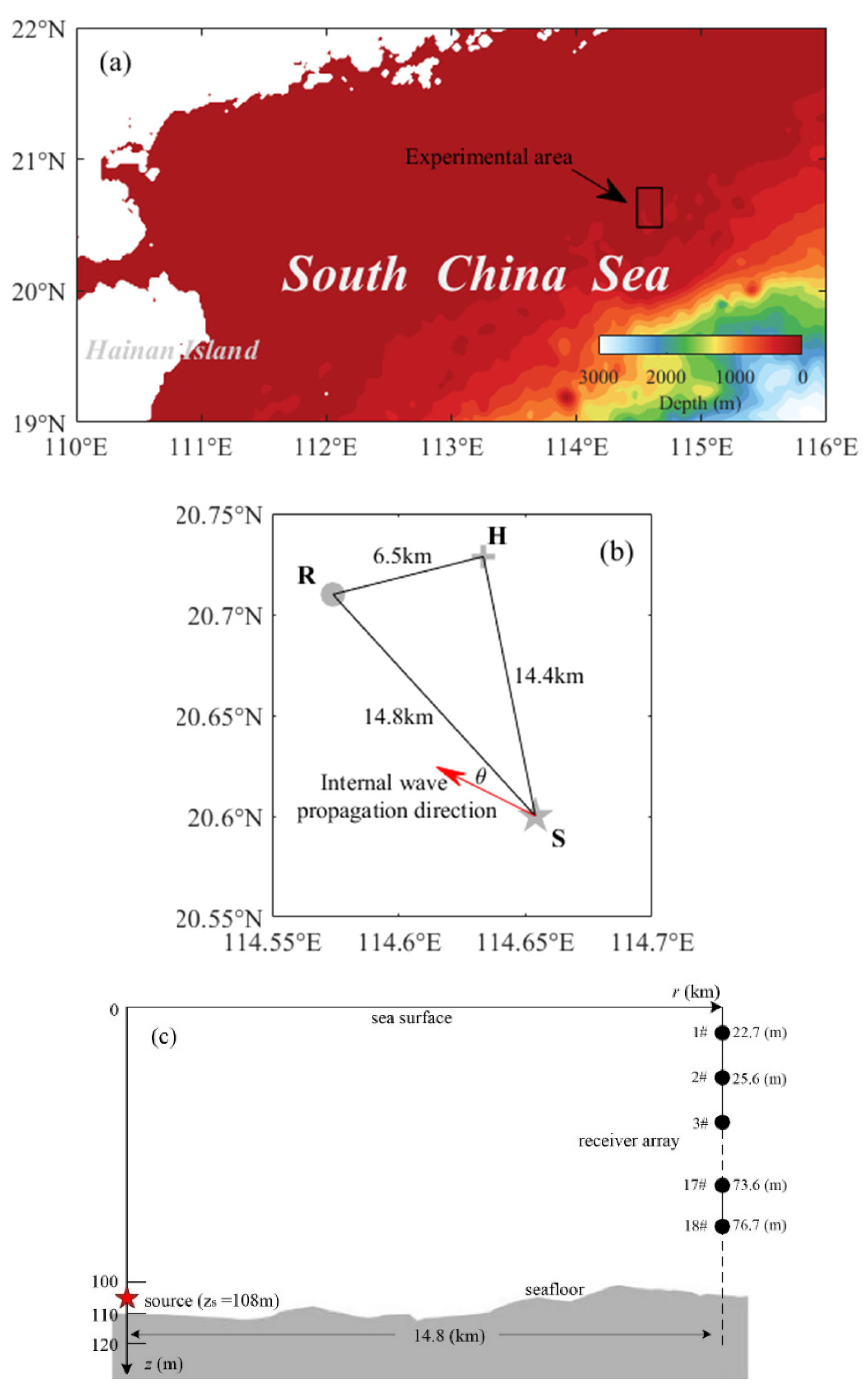
2.2. Acoustic Experiment Descriptions

On 13–17 September 2015, an acoustic propagation experiment was conducted in a continental shelf area in the northern South China Sea. The experiment was to measure the underwater acoustic propagation fluctuations in the internal wave environment. As shown in Figure 1a (The bathymetric data were obtained from the ETOPO1 Global Relief Model [27]), the experimental area is located in the shallow water continental shelf, not far from the continental slope.
Figure 1b presents a top view of the measurement instruments and their locations. The horizontal distances between S and R, S and H, and R and H were 14.8 km, 14.4 km, and 6.5 km, respectively. The acoustic source and vertical line array (VLA) receivers were located at points S and R, respectively. Three VLAs TD sensors were deployed at the points S, R, and H, one each. The three VLAs TD sensors were all deployed at depths of approximately 20 m to 80 m. They were set to record the temperature and depth data once every 30 s, synchronized with the acoustic recording of the VLA receivers. Using the data measured by the three VLAs TD sensors, the average propagation direction and velocity of the internal waves can be obtained. The average horizontal angle θ between the acoustic path SR and the internal waves propagation direction was about 11.17°, and the average propagation speed of the internal waves was about 0.76 m/s. In addition, to obtain full-depth temperature and salinity profile data, 15 measurements of expendable conductivity, temperature, and depth (XCTD) were performed along the acoustic path SR at a horizontal resolution of 1 km.
Figure 1c shows a side view of the bottom bathymetry and the instruments deployed underwater. The bottom topography of the acoustic path SR was almost flat (the bathymetry data are from the multi-beam bathymetry system used during the experiment), with water depths of 110–100 m. The acoustic source and the receiver array were 14.8 km apart. The acoustic source was moored at point S and located at a depth of 108 m, which was 2 m from the bottom. The source transmitted linear frequency-modulated signals at a constant source level with a center frequency of 200 Hz and bandwidth 50 Hz. The signals were 10 s long and were repeated twice every 180 s. The VLA receivers, moored at the point R, consisted of 18 self-capacitating hydrophones spaced approximately 3 m apart, with the first and last hydrophones at depths of 22.7 and 76.7 m, respectively.

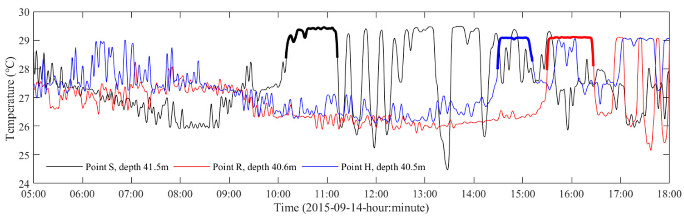
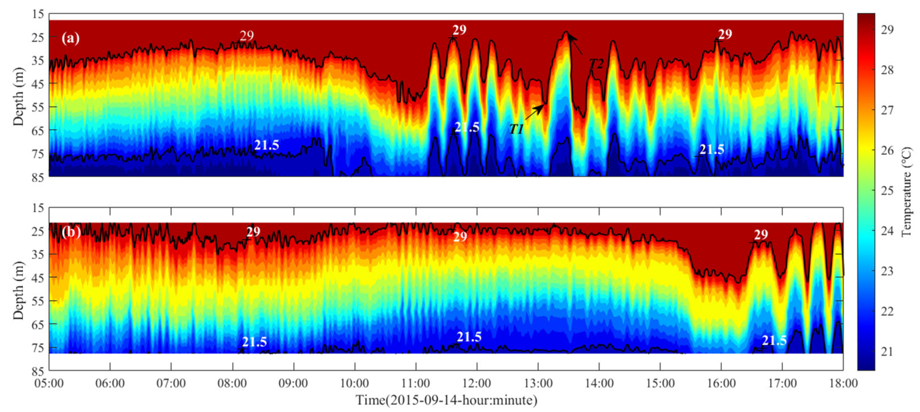
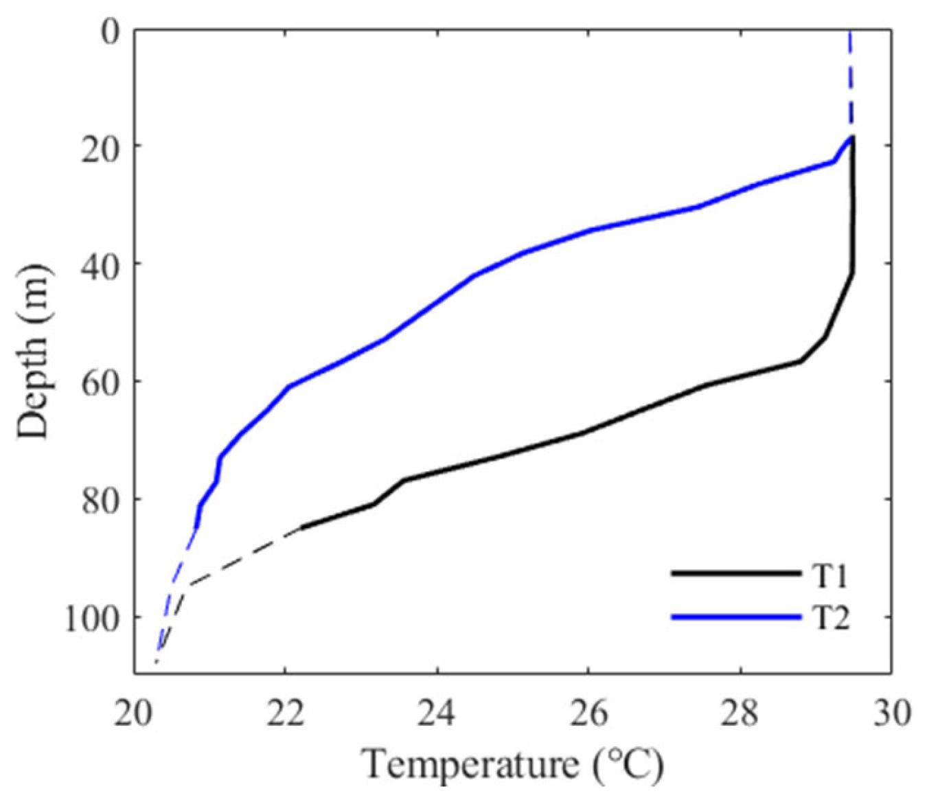
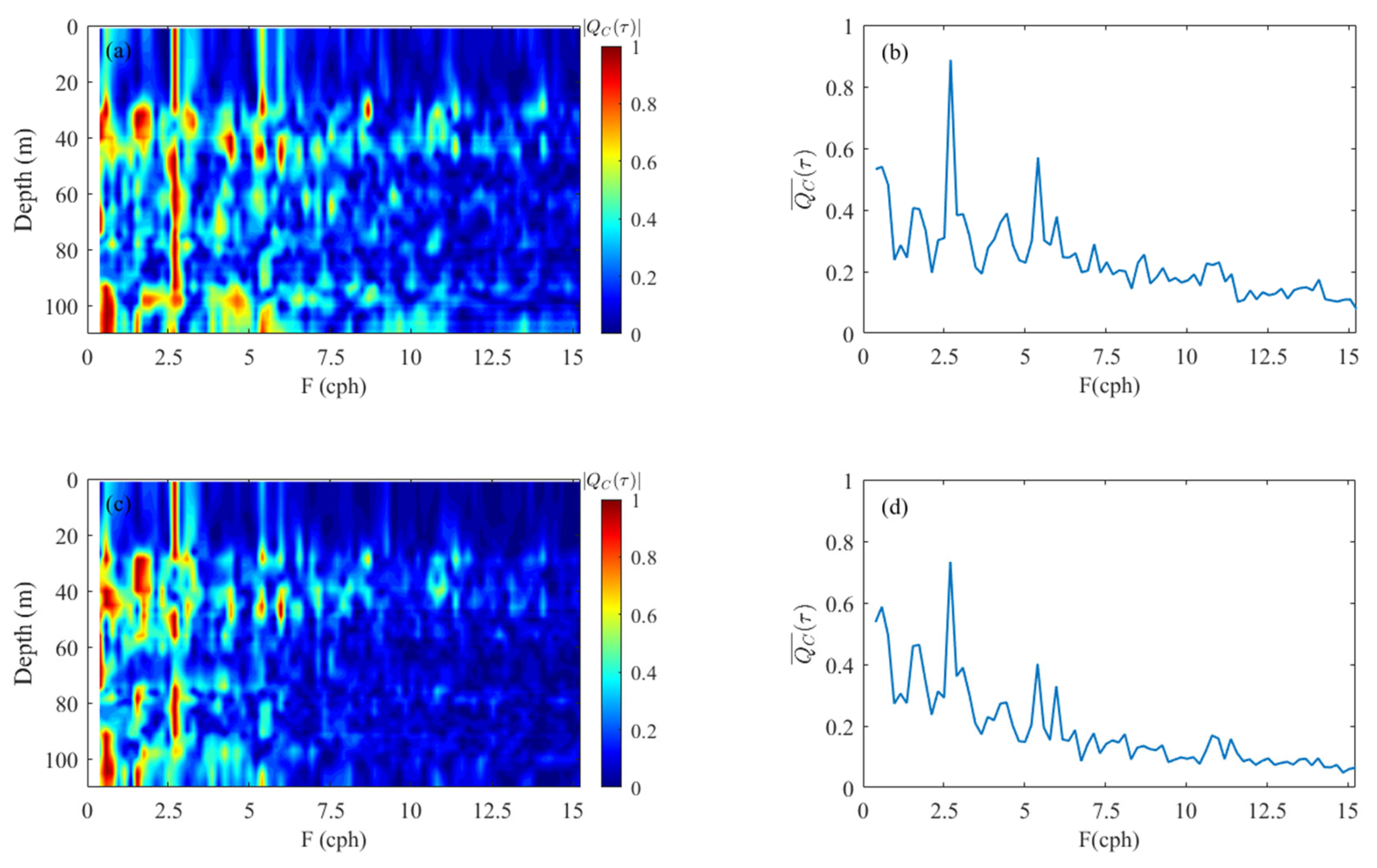
2.3. Internal Wave Analysis

Internal waves are frequent and ubiquitous in the South China Sea, especially in the northern continental shelf and slope areas [1,28]. The reasons can be summarized as the following: (1) the wide shelves and steep slope bathymetry provide conditions for generation and evolution of internal waves; (2) ocean stratification is intensified seasonally by the monsoonal climate; and (3) The Luzon Strait and Taiwan Strait are the main sourse of interal waves. Generally, the internal waves are generated at the continental slope area, and then propagate toward the continental shelf in the northwest direction [29,30,31].
During the acoustic experiment, trains of strong ISWs in the experimental area were recorded by the TD sensors. Figure 2 shows the temperature at time 05:00–18:00 on 14 September 2015, based on the data from the three VLAs TD sensors at similar depths. It is seen that the internal waves cause large fluctuations in the temperature structure of the experimental area. The temporal variations of the temperature can be up to 5 °C over several minutes. At point S, the smaller temperature fluctuations were mainly caused by linear internal waves until about 10:00, after which a train of strong ISWs arrived and caused large temperature fluctuations.
By comparing the bold part of the curves in Figure 2, it can be found that the fronts of the ISWs arrive at the point S first and the point R last, which is in consistent with the propagation direction and average velocity of the internal waves as described in Section 2.2.
The vertical temperature distribution in the experimental area can be characterized as three layers: the surface mixture layer, thermocline layer, and deep layer. The vertical variation in the temperature was small in the surface mixture layer and deep layer, but the temperature decreases downward rapidly from approximately 29 °C to 21.5 °C in the thermocline layer.
Figure 3 shows the filled contour diagrams of temperature versus time and depth at point S and point R. During linear internal wave activity, the thickness of the surface mixed layer was about 30 m, while the depth of the thermocline was up to 75 m. The time length for the ISWs to propagate from the point S to the point R is about 5.48 h. The ISWs caused large fluctuations in the thermocline layer, resulting in variation in the vertical temperature structure (Figure 4).

3. Simulation and Experimental Data Analysis

This section presents the simulation results of acoustic temporal coherence in an ideal ISWs environment and in the acoustic experiment environment. The same geo-acoustic parameters and source-receiver configurations are used in the ideal and experimental environment. The main differences between the two environments are the sound-speed field and bathymetry.

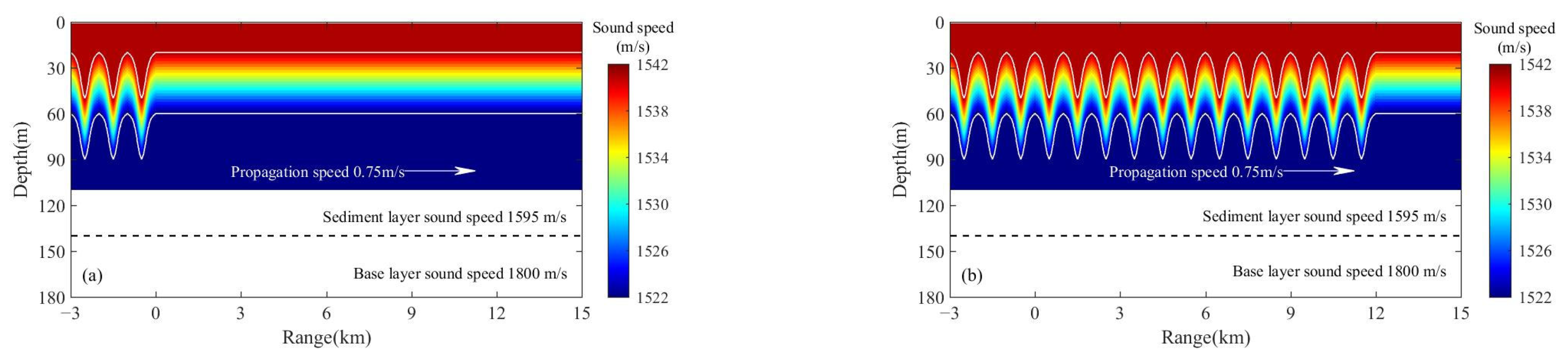
3.1. Simulations in an Ideal ISWs Environment

In the ideal ISWs environment, the depth of the upper boundary of the thermocline   η u ( r , t ) is time-dependent and has the following form [17]:
η u ( r , t ) = sech 2 ( r r 0 + v t Δ ) + η u 0
where , r 0 , v , and Δ are the amplitude, center range, propagation speed, and width of the ISWs, respectively. η u 0 is the depth of the upper boundary of the thermocline without ISWs. The lower boundary of the thermocline is η l ( r , t ) = η u ( r , t )   + 40 m, where 40 m is the thickness of the thermocline. The parameters in Equation (7) were set to   = 30 m, v = 0.75 m/s, Δ = 200 m, and η u 0 = 20 m. The range-dependent sound-speed profile can be described as
c ( r , z ) = { 1542 , 0 < z η u 0 1522 + ( z η u 0 ) * 0.5 , η u 0 < z η u 0 + 40 1522 , η u 0 + 40 < z 110
where z is the depth. The vertical sound-speed gradient of the thermocline was 0.5 s−1. Equations (7) and (8) can be combined to obtain the dynamic sound-speed field in the ideal ISW environment.
The seafloor depth and geo-acoustic parameters were set as range-independent. The seafloor depth was 110 m. A two-layer seafloor was considered. The thickness, sound speed, density, and attenuation coefficient of the sediment layer were 30 m, 1595 m/s, 1700, kg/m3 and 0.39 dB/wavelength, respectively. The sound speed, density and attenuation coefficient of the base layer are 1800 m/s, 2000 kg/m3, and 2.0 dB/wavelength, respectively. The source depth was 108 m. The horizontal and vertical grids for the sound field calculation were set to 4 m and 0.4 m, respectively.
The simulated source was located at r = 0 km, z = 108 m. The frequency band was 175–225 Hz, and the frequency interval used for this band was 2.5 Hz. Figure 5 presents the sound-speed fields at times t   = 0 and t = 4.44 h in the ideal ISWs environment. The interval of the center range r 0 between two ISWs Δ r 0 was set to 1 km. At time t   = 0, the ISWs were in the range r ≤ 0 km. As the ISWs propagated to the right at a constant speed of 0.75 m/s, they passed through the range 0 km and began to appear on the acoustic path. In addition, the shapes of the ISWs were assumed to not change when moving.
Based on the initial range of the ISWs at the time t = 0 and the propagation speed, the front of the ISW arrived at the range of 14.8 km at the time t = 5.48 h. Figure 6 shows the temporal correlation coefficients C ( t , t + τ ) versus time t for three depths (i.e., 12, 48, and 92 m) at the range of 14.8 km over a period of 4.46 h with time delays τ of 0–12 min. C ( t , t + τ ) was calculated by using Equation (6). To highlight the variation characteristics of the large C values, the minimum value for the color bar in the contour plots was set to 0.7. The TCR is a few minutes most of the time. C ( t , t + τ ) does not decrease monotonically with an increasing time delay τ but oscillated, which is consistent with previous studies [21,25]. C was compared at different depths, and C was greater at 92 m than at 12 and 31 m. This implies that fewer acoustic modes contribute to the shallow sound field.
A characteristic of interest is that the temporal variation of the TCR is quasi-periodical, which is more obvious at shallow depths (Figure 6a). It is observed that there are 11 TCR peaks over the 4.44 h period, and the TCR of the peaks can be 12 min or more. The period of the TCR is about 0.372 h, obtained by calculating the average time interval between TCR peaks. In the ideal ISWs environment, the range interval Δ r between two adjacent ISWs is 1 km, and their average propagation speed v is 0.75 m/s. Therefore, the period of the ISW is 0.37 h, which is almost the same as the TCR period.
To show the periodical characteristics of C ( t , t + τ ) more clearly, the temporal correlation coefficient spectrum Q C ( τ ) with a fixed time delay τ can be obtained by using the Fourier transform:
Q C ( τ ) = t 1 t 2 C ( t , t + τ ) e i Ω t d t
where Ω is the angular frequency. The depth-averaged spectrum Q C ¯ ( τ ) = k = 1 K | Q C ( τ ) | / K , where k = 1, 2, …, K . K is the number of depths to be averaged. F = Ω / 2 π is defined as the fluctuation frequency.
Figure 7 presents | Q C ( τ ) | and Q C ¯ ( τ ) at τ = 2 min and 8 min. The highlighted strips indicating the predominant fluctuation frequencies of C ( t , t + τ ) appear in the contour plots (Figure 7a,c). A comparison of | Q C ( τ ) | at different depths shows that the spectral structures are simpler in the shallow layer. The predominant fluctuation frequency can be obtained from the depth-averaged spectra Q C ¯ ( τ ) (Figure 7b,d). It was about 2.71 cycles per hour (cph), which is almost equal to the frequency of the ideal ISWs.
Figure 8 shows the temporal correlation coefficients C ( t , t + τ ) for three depths at the range of 14.8 km with a time delay τ of 0–1.2 h. Three strongly correlated zones can be observed over the 1.2 h time delay, which are marked with rectangles in the contour plots (Figure 8a,c,e). It is shown that C ( t , t + τ ) at different time t can reach local maximum values with roughly the same τ . In addition, the strongly correlated zones are located with approximately the same τ at different receiver depths.
The strongly correlated zones correspond to the inflection points of the time-averaged correlation coefficient C t ¯ ( τ ) curves, which are marked with “x” symbols on the average curves (Figure 8b,d,f). The time-averaged correlation coefficient was calculated as C t ¯ ( τ ) = j = 1 J | Q C ( τ ) | C ( t j , t j + τ ) / J , where j = 1, 2, …, J , and J is the number of time moments to be averaged. One observes that there are three inflection points over the 1.2 h time delay, and τ of the first, second, and third inflection point is about 0.37 h, 0.74 h, and 1.11 h, respectively. C t ¯ ( τ ) at different inflection points are not the same, and their overall trends are to decrease with τ .
It is found that the time delay intervals Δ τ between two adjacent inflection points are 0.37 h, and remain approximately the same at different receiver depths. If Δ τ is assumed to be the oscillation period of the temporal correlation curves, it can be concluded that C t ¯ ( τ ) varies quasi-periodically with the time delay τ . Thus, the periods of the C t ¯ ( τ ) curves and the ISWs are also the same.

3.2. Simulations in the Experiment Environment and Verification with Experimental Data

The main challenge, to construct the environmental model approximating the real experimental conditions in the actual ocean, is obtaining the sound-speed field along the acoustic path. This is because the ISW environment is range-dependent and time-varying. To construct the experimental environment model for acoustic simulation, the temperature profiles measured by the VLA TD sensors at point R are the used to provide time-varying sound-speed field in the water column.
An important assumption is that the shape of the ISWs train is invariant as it moves. Thus, the temperature profiles measured at different times correspond to different ranges according to the average propagation speed of the ISWs. The salinity profile used to calculate the sound speed was derived from the XCTD probes. Because the sound speed is less affected by the salinity in shallow water, the salinity profile is assumed to be range-independent and time-invariant. Figure 9 shows two snapshots of the sound speed fields at the times t = 0 and t = 2.75 h. At time t = 0, only linear internal waves with a small amplitude appear on the acoustic path. After time t = 0, a train of strong ISWs propagates along the acoustic path through the source (r = 0 km), which leads to sound field fluctuations.
Figure 10 shows the sound speed c, time gradient of sound speed c’, and depth-averaged correlation coefficient C d ¯ ( t , t + τ ) over a period of 2.75 h. The temporal gradient of the sound speed was calculated as c ( t ) = [ c ( t + Δ t ) c ( t ) ] / Δ t , where Δ t = 30 s is equal to the measurement resolution of the TD sensors. The depth-averaged correlation coefficient C d ¯ ( t , t + τ ) = k = 1 K C k ( t , t + τ ) / K , where k = 1, 2, …, K and K is the number of depths to be averaged.
It is seen that there are eight ISWs passing through point R during this time period (Figure 10a), and the ISWs have irregular shapes that are different from each other. The ISWs induce significant temporal gradient in the sound-speed fields c ( t ) (Figure 10b). c ( t ) can be converted into the horizontal gradient c ( r ) based on the average propagation speed of the ISW train. In a range-dependent environment, c ( r ) results in mode coupling [5,32,33,34], which is the main physical mechanism causing fluctuations in the sound field and temporal acoustic coherence. Figure 10c shows the depth-averaged temporal correlation coefficients for 1 m to 20 m versus time and time delay, because the spectrum structures in the shallow layer are relatively simpler as noted in Section 3.1. The TCR is about a few minutes most of the time. In addition, eight small TCR segments can be observed in the depth-averaged (1–20 m) contour plot corresponding to the eight ISWs. The variation period of the TCR is generally consistent with that of the ISWs.
Figure 11 shows the temporal correlation coefficients C ( t , t + τ ) obtained from the experimental data of two receivers at depths of 31.4 m and 61.6 m, over a period of 2.75 h, with time delays τ of 0–12 min. C ( t , t + τ ) was calculated by using Equation (4). The time period in Figure 11 is the same as that in Figure 10. As can be seen from Figure 11, TCR is about a few minutes most of the time, and C ( t , t + τ ) oscillates significantly with time t and delay τ .
In the real experiment environment, the structures of the dynamic ISWs along the acoustic path are not perfectly known, as their shapes change with movement. In addition, the uncertainties in sea-surface motion, geo-acoustic parameters and source-receiver geometry can also lead to fluctuations in sound field and temporal coherence. Therefore, C ( t , t + τ ) from the experimental data (Figure 11a) are not in perfect agreement with the simulation results (Figure 6b and Figure 10). Figure 12 presents the correlation coefficient C ( t , t + τ ) of a fixed time delay τ = 3 min at roughly the same depth of 31 m. One observes that the general tendency of C ( t , t + τ ) are similar. However, it is not enough to make an explicit statement about the oscillation period of C ( t , t + τ ) .

4. Discussion

The temporal correlation coefficients were derived from the time-varying sound field. In order to provide an interpretation for the characteristics of the quasi-periodic acoustic temporal coherence, the temporal fluctuations of the sound field in the ISWs environment and the associated physical mechanisms need to be analyzed.

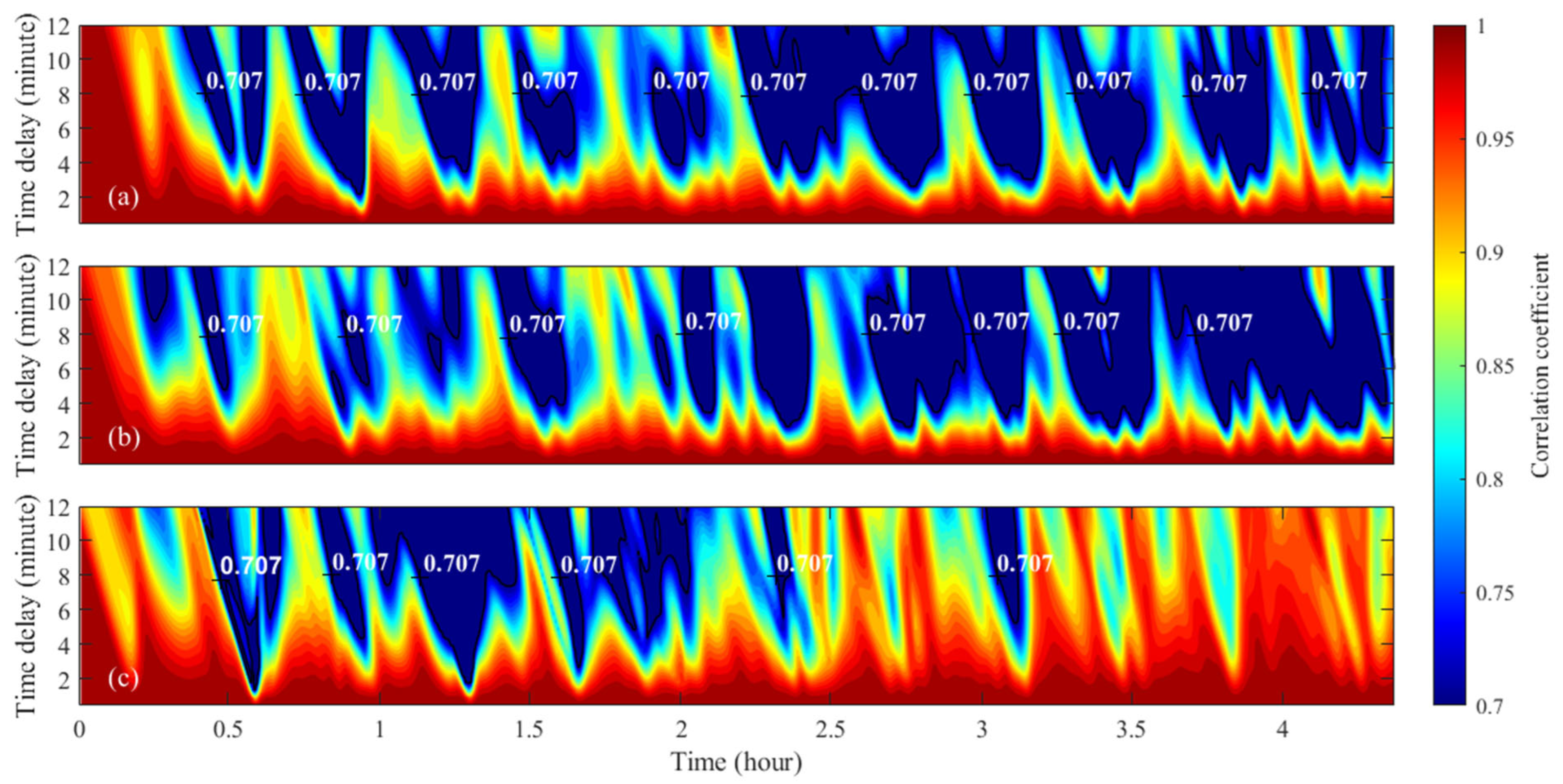
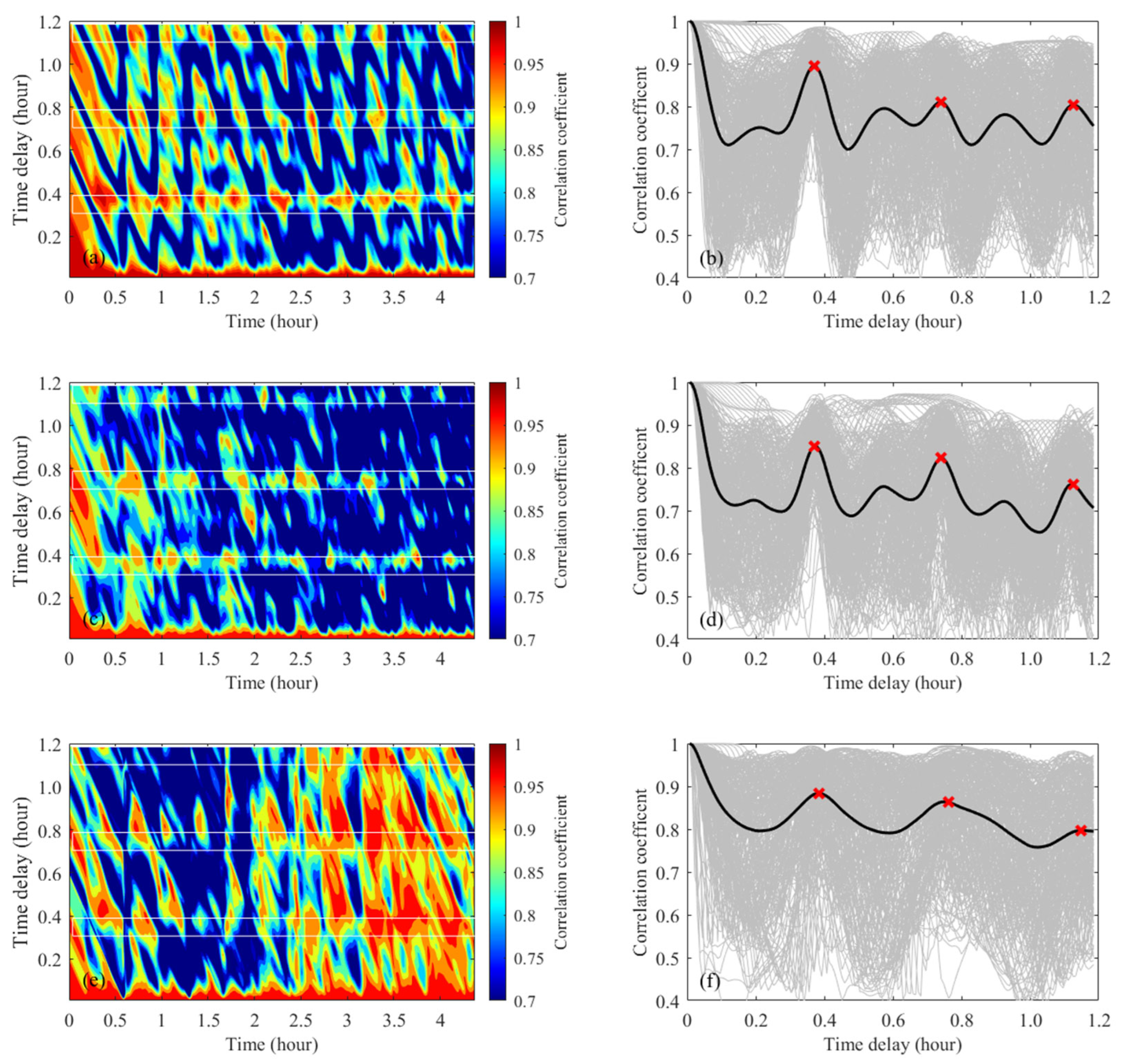
4.1. Quasi-Periodical Sound Field in the ISWs Environment

The complex sound pressure p of the frequency f at point ( r , z ) can be given in the form of the product of the amplitude A and phase .
p r , z , f ( t ) = A r , z , f ( t ) e i r , z , f ( t )
In a dynamic internal wave environment, p , A, and are time-varying parameters. By substituting Equation (10) into Equation (6), the temporal correlation coefficient C ( t , t + τ ) becomes
C ( t , t + τ ) = max 0 n = 1 N A f n ( t ) A f n ( t + τ ) [ cos f n ( t , t + τ ) ] ( n = 1 N A f n 2 ( t ) n = 1 N A f n 2 ( t + τ ) ) 1 / 2
where
f n ( t , t + τ ) = f n ( t ) f n ( t + τ ) + 0
The subscripts r and z are dropped for brevity. R e [ e i f n ( t , t + τ ) ] = cos [ f n ( t , t + τ ) ] . Equation (11) indicates that C ( t , t + τ ) is mainly affected by the amplitude and the phase. Let A(t) = [ A f 1 ( t ) ,   A f 2 ( t ) ,…, A f N ( t ) ]. Then, a smaller standard deviation of A(t) results in a larger C ( t , t + τ ) . Meanwhile, cos [ f n ( t , t + τ ) ] is controlled by the correction term 0 . A smaller f n ( t , t + τ ) (i.e., the smaller difference between f n ( t ) and f n ( t + τ ) after phase correlated by 0 ) results in a larger C ( t , t + τ ) .
Figure 13 shows the amplitude A f ( t ) and the phase f ( t ) of the complex sound pressure at the range of 14.8 km and depth of 12 m in the ideal ISWs environment, corresponding to the temporal correlation coefficients shown in Figure 6a. One sees that the temporal variations of both A f ( t ) and f ( t ) are quasi-periodical, while the temporal variations of different frequencies are not the same.
To show the temporal fluctuations of the sound field more clearly, the spectra were calculated. First, the temporal correlation coefficient C ( t , t + τ ) in Equation (9) was replaced with the complex sound pressure p f ( t ) , amplitude A f ( t ) , and phase f ( t ) to obtain the spectra Q f , p , Q f , A , and Q f , , respectively. Then, the frequency-averaged spectra Q p , Q A , and Q were obtained by averaging over the frequency band. Finally, the depth-averaged spectra Q p ¯ , Q A ¯ , and Q ¯ are calculated using the frequency-averaged spectra. The normalized frequency-averaged spectra and depth-averaged spectra are presented in Figure 14.
The highlight strips in the contour plots (Figure 14a,c,e) indicate the remarkable fluctuation frequencies of the sound field. The strips correspond to the peaks on the depth-averaged curves (Figure 14b,d,f). Among the spectra of Q p ( Q p ¯ ), Q A ( Q A ¯ ), and Q ( Q ¯ ), Q p ( Q p ¯ ) is more similar to Q A ( Q A ¯ ), which indicates that the amplitude is the predominant factor that affects the fluctuation frequencies of the complex sound field.
The highlight strips in Figure 14a have similar distribution characteristics to those in Figure 7a,c. There are three remarkable peaks in the depth-averaged curves Q p ¯ in Figure 14b, and the frequencies of the first, second, and third peaks are 1.08 cph, 2.16 cph, and 2.7 cph, respectively. By comparing to the fluctuation frequencies of the temporal correlation efficient in Figure 7, it is found that the third peak of Q p ¯ corresponds well with the fluctuation frequencies of the temporal coherence.

4.2. Mechanism Interpretation Using Coupled Normal Mode Theory

In the range-dependent environment shown in Figure 15, a train of ISWs propagate from the source to the VLA receivers at a constant speed v . The medium is range-dependent and time-varying within the region 0 < r   r J , and it is range-independent and time-invariant within the region r J   < r   r J + 1 .
The range-dependent region 0 < r r J is subdivided equally into J segments, and the medium within each within each segment is assumed to be range-independent. The range-independent region r J   < r   r J + 1 is treated as one segment. According to the coupled normal modes theory, the sound pressure received at the (J + 1)th segment can be expressed as [17].
p J + 1 ( r , z ) = r J / r m = 1 M a m J + 1 h m J + 1 ( r ) m J + 1 ( z )
where m = 1, 2, …, M and M is the mode number. The local eigenfunction m J + 1 ( z ) and eigenvalue k m J + 1 can be obtained from the local equation ρ 0 [ / z ( ρ 0 1 m J + 1 / z ) ] + [ ω 2 / c J + 1 2 ( z ) ( k m J + 1 ) 2 ] m J + 1 = 0 , where c J + 1 ( z ) is the local sound-speed profile in the (J + 1)th segment. ρ 0 is the density, and ω is the angular frequency. Approximation of the Hankel functions by asymptotic form yields.
h m J + 1 ( r ) = e x p [ i k m J + 1 ( r r J ) ]
If a mode coefficient vector a(t) = [ a 1 J + 1 ( t ) ,   a 2 J + 1 ( t ) ,…, a M J + 1 ( t ) ] is assumed, and h J + 1 ( r )   is a M × M diagonal matrix with elements h m J + 1 ( r ) defined in Equation (14), then these mode coefficients can be obtained by using those in the preceding segments [18].
a J + 1 = r / r J R a 1
Here, a 1 is the initial coefficient vector and R is the transmission matrix:
a m 1 = 1 / k m 1 m 1 ( z s ) exp ( i k m 1 r 1 )
R = C J h J ( r J ) C J 1 h J 1 ( r J 1 ) C 1 h 1 ( r 1 )
where R and C J are M × M propagation and coupling matrices, and their elements are propagation coefficient R m n and coupling coefficient c m n J ( = 0 ρ 0 ( z ) m J + 1 ( z ) n J ( z ) d z ) , respectively. In a range-independent environment, R and C J are diagonal matrices (i.e., R m n = 0 and c m n J = 0 when mn). In a range-dependent environment, R m n   ≠ 0 and c m n J   ≠ 0 when mn.
In the simulation environment, the range between the source and receiver VLA is a constant r e = 14.8 km (i.e., r J + 1 = 14.8 km). If r 1 r 0   = 1 m, then, the sound field at r e can be written as
p ( r e , z ) = m = 1 M 1 / ( k m J + 1 r e ) h m J + 1 ( r J + 1 ) m J + 1 ( z ) ( n = 1 M R m n a n 1 )
For the traveling ISWs environment in Figure 15, the three main influences responsible for the quasi-periodical fluctuations of the sound field are the initial sound field a n 1 , the acoustic propagation factor R m n , and the phase factor h m J + 1 ( r J + 1 ) .
As the ideal ISWs train propagates across the range r 0 to the acoustic path, the initial mode amplitudes m 1 ( z s = 108   m ) and mode eigenvalues k m 1 vary periodically, which leads to periodical initial sound field a m 1 according to Equation (16). Internal waves are known to cause acoustic mode coupling and energy transfer between modes [6,8]. As more ISWs propagate through the source at the range r 0 to the acoustic path, the range-dependent range r J + 1 increases while the range-independent range Δ r 0 (=   r e     r J ) decreases. Therefore, the propagation matrix R and phase matrix h J + 1 ( r J + 1 ) are time-dependent functions. Thus, separating the influences that cause the temporal fluctuations of the sound field shown in Figure 14b is difficult.
Previous studies [16,17,34] reported that all the ISWs in the train enter the acoustic path and move along it. The medium at the source and receivers is range-independent and unaffected by the ISWs. Therefore, the initial modes excited at the source are time-invariant, and the propagation and phase matrices are independent of the ISW positions on the acoustic path.
According to Equation (18), the sound field comprises M modes, and the amplitude of a single mode is given by b m ( r e ) = 1 / ( k m J + 1 r e ) n = 1 M R m n a n 1 . Figure 16 shows the mode amplitude versus time at the range of 14.8 km. One sees that the mode amplitudes versus time displays a structure with abundant variations. The mode amplitude decreases with the mode order, and the first seven modes contribute most of the energy to the sound field at the range of 14.8 km.
Replacing the temporal correlation coefficient C ( t , t + τ ) in Equation (9) with the mode amplitude b m ( r e ) obtains the spectrum Q ( b m ) , as shown in Figure 17. The fluctuation frequencies vary greatly with the mode number. Not all the mode fluctuations have significant predominant frequencies, which indicate that the sound field fluctuations result from some specific modes. A comparison between the spectra of the sound pressure in Figure 14b and the mode amplitude in Figure 17 indicates that the peaks in Figure 14b result from different modes. The temporal fluctuations of mode 2 and mode 3 are responsible for the first peak in Figure 14b, while the temporal fluctuations of mode 4 and mode 5 are responsible for the second and third peaks in Figure 14b. The temporal fluctuations of the mode amplitudes in the ideal ISWs environments are also caused by the initial sound field a n 1 , the acoustic propagation factor R m n , and the phase factor h m J + 1 ( r J + 1 ) . No further discussions are provided in this paper.
Figure 18 shows the local eigenfunctions m at the range of 14.8 km. The amplitude of the real part of m in the shallow layer (or the mixture layer above thermocline) is small for modes 1–3. Therefore, modes 1–3 contribute very little to the shallow layer sound field. On the other hand, the higher-order modes also contribute little because they attenuate rapidly with the propagation range. As a result, the sound field interference in the shallow layer results from fewer modes than in the deep layer, which leads to the simpler spectrum structures in the shallow layer in Figure 17a,c.

5. Conclusions

This study focused on the temporal coherence of the low-frequency (175–225 Hz) sound field in a shallow-water ISW environment characterized by ISWs continuously passing the acoustic source and approaching receivers along the acoustic path. Broadband acoustic simulations were performed in an ideal ISW environment, and the results were compared with those obtained in an experimental environment. The broadband simulation results were generally consistent with the experimental data. The Fourier transform method was used to obtain the temporal fluctuation frequencies of the temporal correlation coefficients C ( t , t + τ ) and the sound field, and the related physical mechanisms were discussed by using the coupled normal mode theory.
Two key features of the acoustic temporal coherence are obtained as follows: (1) C ( t , t + τ ) with the same time delay τ that is smaller than the TCR oscillates quasi-periodically with the time t ; (2) C ( t , t + τ ) with the same t also oscillates quasi-periodically with the time delay τ . The predominant oscillation periods are equal to the ISW period. The periodicity of the temporal correlation coefficients results from the quasi-periodic sound field, which is mainly caused by some specific acoustic modes. There are fewer effective modes in the shallow layer than in the deep layer, which results in simpler sound field interference structures and fluctuation spectrum structures in the shallow layer.
In a dynamic ISW environment, two major physical mechanisms are responsible for the quasi-periodic sound field fluctuations: the initial sound field excited at the source and the mode coupling. The ISWs continuously passing the acoustic source induce periodic initial acoustic modes and sound fields. The effects of the mode coupling can be described by a time-varying acoustic propagation matrix and phase matrix as more ISWs propagate along the acoustic path over time.
It should be noted that the mode coupling and the temporal variation of mode amplitude in the environment scenario in this study is complex. Therefore, the study was focused on the predominant fluctuation frequencies of the sound fields and the acoustic modes without providing the interpretation for the abundant variation structure of the mode amplitudes. Meanwhile, the ISWs can affect the underwater acoustic communications because they result in fluctuations in the sound field and acoustic temporal coherence. The underwater communication performance in the internal wave environment is a significant topic.

Author Contributions

Conceptualization, F.X., Z.L. and J.Q.; methodology, F.G., P.H. and J.Q.; formal analysis, F.G. and P.H.; investigation, Z.L. and J.Q.; resources, J.Q.; writing—original draft preparation, F.G. and P.H.; writing—review and editing, F.X., Z.L. and J.Q.; supervision, F.X., Z.L. and J.Q.; funding acquisition, F.X., Z.L. and J.Q. All authors have read and agreed to the published version of the manuscript.

Funding

This research was funded by the National Key Research and Development Program of China, grant number 2020YFA0607900; the National Natural Science Foundation of China, grant number 42176019 and 11874061; the Youth Innovation Promotion Association CAS, grant number 2021023.

Institutional Review Board Statement

Not applicable.

Informed Consent Statement

Not applicable.

Data Availability Statement

Not applicable.

Acknowledgments

The experiment data of acoustic propagation in internal wave environment was from Institute of Acoustics in Chinese Academy of Sciences.

Conflicts of Interest

The authors declare no conflict of interest.

References

  1. Zheng, Q.A.; Xie, L.L.; Xiong, X.J.; Hu, X.M.; Chen, L. Progress in research of submesoscale processes in the South China sea. Acta Oceanol. Sin. 2020, 39, 1–13. [Google Scholar] [CrossRef]
  2. Wang, J.F.; Yu, F.; Nan, F.; Ren, Q.; Chen, Z.F.; Zheng, T.T. Observed three dimensional distributions of enhanced turbulence near the Luzon Strait. Sci. Rep. 2021, 11, 14835. [Google Scholar] [CrossRef] [PubMed]
  3. Whalen, C.B.; de Lavergne, C.D.; Garabato, A.C.N.; Klymak, J.M.; MacKinnon, J.A.; Sheen, K.L. Internal wave-driven mixing: Governing processes and consequences for climate. Nat. Rev. Earth Environ. 2020, 1, 606–621. [Google Scholar] [CrossRef]
  4. Apel, J.R.; Ostrovsky, L.A.; Stepanyants, Y.A.; Lynch, J.F. Internal solitons in the ocean and their effect on underwater sound. J. Acoust. Soc. Am. 2007, 121, 695–722. [Google Scholar] [CrossRef]
  5. Lynch, J.F.; Lin, Y.-T.; Duda, T.F.; Newhall, A.E. Acoustic ducting, reflection, refraction, and dispersion by curved nonlinear internal waves in shallow water. IEEE J. Ocean. Eng. 2010, 35, 12–27. [Google Scholar] [CrossRef]
  6. Dossot, G.A.; Smith, K.B.; Badiey, M.; Miller, J.H.; Potty, G.R. Underwater acoustic energy fluctuations during strong internal wave activity using a three-dimensional parabolic equation model. J. Acoust. Soc. Am. 2019, 146, 1875. [Google Scholar] [CrossRef]
  7. Zhou, J.X.; Zhang, X.Z.; Rogers, P.H. Resonant interaction of sound wave with internal solitons in the coastal zone. J. Acoust. Soc. Am. 1991, 90, 2042–2054. [Google Scholar] [CrossRef]
  8. Preisig, J.C.; Duda, T.F. Coupled acoustic mode propagation through continental-shelf internal solitary waves. IEEE J. Ocean. Eng. 1997, 22, 256–269. [Google Scholar] [CrossRef]
  9. Duda, T.F. Acoustic mode coupling by nonlinear internal wave packets in a shelfbreak front area. IEEE J. Ocean. Eng. 2004, 29, 118–125. [Google Scholar] [CrossRef]
  10. Gao, F.; Xu, F.H.; Li, Z.L.; Qin, J.X. Mode coupling and intensity fluctuation of sound propagation over continental slope in presence of internal waves. Acta Phys. Sin. 2022, 71, 204301–204314. (In Chinese) [Google Scholar] [CrossRef]
  11. Katsnel’son, B.G.; Pereselkov, S.A. Low-frequency horizontal acoustic refraction caused by internal wave solitons in a shallow sea. Acoust. Phys. 2000, 46, 684–691. [Google Scholar] [CrossRef]
  12. Badiey, M.; Katsnelson, B.G.; Lynch, J.F.; Pereselkov, S.; Siegmann, W.L. Measurement and modeling of three-dimensional sound intensity variations due to shallow-water internal waves. J. Acoust. Soc. Am. 2005, 117, 613–625. [Google Scholar] [CrossRef]
  13. Lin, Y.; Duda, T.F.; Lynch, J.F. Acoustic mode radiation from the termination of a truncated nonlinear internal gravity wave duct in a shallow ocean area. J. Acoust. Soc. Am. 2009, 126, 1752–1765. [Google Scholar] [CrossRef] [PubMed]
  14. Frank, S.D.; Badiey, M.; Lynch, J.F.; Siegmann, W.L. Experimental evidence of three-dimensional acoustic propagation caused by nonlinear internal waves. J. Acoust. Soc. Am. 2005, 118, 723–734. [Google Scholar] [CrossRef]
  15. Katsnelson, B.G.; Grigorev, V.; Badiey, M.; Lynch, J.F. Temporal sound field fluctuations in the presence of internal solitary waves in shallow water. J. Acoust. Soc. Am. 2009, 126, EL41–EL48. [Google Scholar] [CrossRef]
  16. Qin, J.X.; Katsnel’son, B.G.; Li, Z.L.; Zhang, R.H.; Luo, Y.W. Intensity fluctuations due to the motion of internal solitons in shallow water. Acta Acust. 2016, 41, 145–153. (In Chinese) [Google Scholar] [CrossRef]
  17. Rouseff, D.; Turgut, A.; Wolf, S.N.; Finette, S.; Orr, M.H.; Pasewark, B.H.; Apel, J.R.; Badiey, M.; Chiu, C.S.; Headrick, R.H.; et al. Coherence of acoustic modes propagating through shallow water internal waves. J. Acoust. Soc. Am. 2002, 111, 1655–1666. [Google Scholar] [CrossRef]
  18. Li, Q.R.; Sun, C.; Xie, L. Research on the modal intensity fluctuation during the dynamic propagation of internal solitary waves in the shallow water. Acta Phys. Sin. 2022, 71, 024302-1-13. (In Chinese) [Google Scholar] [CrossRef]
  19. Headrick, R.H.; Lynch, J.F.; Kemp, J.N.; Newhall, A.E.; von der Heydt, K.; Apel, J.; Badiey, M.; Chiu, C.; Finette, S.; Orr, M.; et al. Acoustic normal mode fluctuation statistics in the 1995 SWARM internal wave scattering experiment. J. Acoust. Soc. Am. 2000, 107, 201–220. [Google Scholar] [CrossRef] [PubMed]
  20. Yang, T.C. Measurements of temporal coherence of sound transmissions through shallow water. J. Acoust. Soc. Am. 2006, 120, 2595–2614. [Google Scholar] [CrossRef]
  21. Ji, G.; Zhi, J.; Yong-Bo, S.; Wei, C.; Xian-Tai, W.; Gao-Peng, C.; Xin-Yu, L. A Physics-Based Charge-Control Model for InP DHBT Including Current-Blocking Effect. Chin. Phys. Lett. 2009, 26, 077302. [Google Scholar] [CrossRef]
  22. Duda, T.F. Temporal and cross-range coherence of sound traveling through shallow-water nonlinear internal wave packets. J. Acoust. Soc. Am. 2006, 119, 3717–3725. [Google Scholar] [CrossRef]
  23. Lunkov, A.A.; Petnikov, V.G. The coherence of low-frequency sound in shallow water in the presence of internal waves. Acoust. Phys. 2014, 60, 61–71. [Google Scholar] [CrossRef]
  24. Yoo, K.B.; Yang, T.C. Broadband source localization in shallow water in the presence of internal waves. J. Acoust. Soc. Am. 1999, 106, 3255–3269. [Google Scholar] [CrossRef]
  25. Yoo, K.B. Shallow water temporal coherence of broadband acoustic signals in the presence of internal waves. IEEE J. Ocean. Eng. 2005, 30, 391–405. [Google Scholar] [CrossRef]
  26. Collins, M.D. A split-step Padé solution for the parabolic equation method. J. Acoust. Soc. Am. 1993, 93, 1736–1742. [Google Scholar] [CrossRef]
  27. Amante, C.; Eakins, B.W. ETOPO1 1 arc-minute global relief model: Procedures, data sources and analysis. Psychologist 2009, 16, 20–25. [Google Scholar]
  28. Guo, C.C.; Chen, X.E. A review of internal solitary wave dynamics in the northern South China Sea. Prog. Oceanogr. 2014, 121, 7–23. [Google Scholar] [CrossRef]
  29. Wang, J.; Huang, W.G.; Yang, J.S.; Zhang, H.G.; Zheng, G. Study of the propagation direction of the internal waves in the South China sea using satellite imagines. Acta Oceanol. Sin. 2012, 32, 42–50. [Google Scholar] [CrossRef]
  30. Li, D.; Chen, X.; Liu, A. On the generation and evolution of internal solitary waves in the northwestern South China sea. Ocean Model. 2011, 40, 105–119. [Google Scholar] [CrossRef]
  31. Zheng, Q. Satellite SAR Detection of Sub-Mesoscale Ocean Dynamic Processes; World Scientific Publishing Co. Inc.: Singapore, 2017. [Google Scholar]
  32. Dozier, L.B.; Tappert, F.D. Statistics of normal mode amplitudes in a random ocean. I. Theory. J. Acoust. Soc. Am. 1978, 63, 353–365. [Google Scholar] [CrossRef]
  33. Liu, J.Q.; Piao, S.C.; Gong, L.J.; Zhang, M.H.; Guo, Y.C.; Zhang, S.Z. The effect of mesoscale eddy on the characteristic of sound propagation. J. Mar. Sci. Eng. 2021, 9, 787. [Google Scholar] [CrossRef]
  34. Jiang, Y.Y.; Grigorev, V.; Katsnelson, B. Sound field fluctuations in shallow water in the presence of moving nonlinear internal waves. J. Mar. Sci. Eng. 2022, 10, 119. [Google Scholar] [CrossRef]
Figure 1. Acoustic experiment: (a) location of the experimental area and bathymetric contours, (b) geometry for the measurement positions of the deployed instruments (top view), (c) geometry for the positions of the acoustic source and VLA hydrophones (side view).
Jmse 11 00374 g001
Figure 2. Temperature versus time measured at points S (black), R (red), and H (blue).
Jmse 11 00374 g002
Figure 3. Temperature versus time and depth measured at points (a) S and (b) R.
Jmse 11 00374 g003
Figure 4. Temperature versus depth measured at different times. The solid curves are from the data of VLA TD sensors, and the dashed curves are added using the data of the XCTD probe.
Jmse 11 00374 g004
Figure 5. Background sound-speed fields for acoustic simulation at different times: (a) t = 0 and (b) t = 4.44 h. The sound-speed fields are constructed based on Equations (7) and (8).
Jmse 11 00374 g005
Figure 6. Contour plots of simulated correlation coefficients vs. time and time delay at the range of 14.8 km in the ideal ISWs environment at three different depths: (a) 12 m, (b) 31 m, and (c) 92 m.
Jmse 11 00374 g006
Figure 7. Spectra of C ( t , t + τ ) with different time delays τ : (a,b) τ = 2 min and (c,d) τ = 8 min. The left panels show contour plots of the normalized spectra | Q C ( τ ) | versus the depth and fluctuation frequency F . The right panels show the curves of depth-averaged spectra Q C ¯ ( τ ) versus F .
Jmse 11 00374 g007
Figure 8. Simulated correlation coefficients at the range of 14.8 km in the ideal ISWs environment at three different depths: (a,b) 12 m, (c,d) 31 m, and (e,f) 92 m. The left three panels show contour plots of correlation coefficients vs. the time and time delay, and the rectangles mark the strongly correlated zones. The right three panels show curves of correlation coefficients vs. the time delay at different times. The bold curve is the time-averaged correlation coefficients, and the “x” symbols mark the inflection points.
Jmse 11 00374 g008
Figure 9. Sound-speed fields constructed for simulation at different times: (a) t = 0 and (b) t = 2.75 h. The sound-speed fields are measured by the VLA TD sensors at point R.
Jmse 11 00374 g009
Figure 10. Contour plots of the (a) measured sound speed, (b) sound-speed gradient, (c) simulated depth-averaged (1–20 m) temporal correlation coefficient, and (d) simulated temporal correlation coefficient at depth 31 m, over a 2.75-h period.
Jmse 11 00374 g010
Figure 11. Contour plots of correlation coefficients vs. time and time delay measured in the experiment at two different depths: (a) 31.4 m and (b) 61.6 m.
Jmse 11 00374 g011
Figure 12. Correlation coefficient C ( t , t + τ ) versus time t of a fixed time delay τ = 3 min. C 1 are simulated results obtained from Figure 6b, C 2 are simulated results obtained from Figure 10d, and C 3 are measured results obtained from Figure 11a.
Jmse 11 00374 g012
Figure 13. Contour plots of the simulated sound pressure phase and amplitude versus frequency and time. (a) the phase f ( t ) and (b) the amplitude A f ( t ) .
Jmse 11 00374 g013
Figure 14. Spectra of the (a,b) complex sound pressure, (c,d) amplitude, and (e,f) phase. The left panels show contour plots of the normalized frequency-averaged spectra versus depth and fluctuation frequency F. The right panels show curves of depth-averaged spectra versus F. The three peaks of depth-averaged curves Q p ¯ is marked with red cross.
Jmse 11 00374 g014
Figure 15. Source-receiver geometry with a train of traveling ISWs.
Jmse 11 00374 g015
Figure 16. Mode amplitude b m ( r e ) versus time for modes 1, 3, and 7.
Jmse 11 00374 g016
Figure 17. Spectra of mode amplitudes b m ( r e ) for modes 1–7.
Jmse 11 00374 g017
Figure 18. Real part of the local mode eigenfunctions m for modes 1–7.
Jmse 11 00374 g018
Disclaimer/Publisher’s Note: The statements, opinions and data contained in all publications are solely those of the individual author(s) and contributor(s) and not of MDPI and/or the editor(s). MDPI and/or the editor(s) disclaim responsibility for any injury to people or property resulting from any ideas, methods, instructions or products referred to in the content.

