Variational Bayesian Inference Time Delay Estimation for Passive Sonars

Abstract

In passive sonars, distance and depth estimation of underwater targets is often limited by the accuracy of time delay estimations. The estimation accuracy of the existing methods of time delay estimation is limited by the uniform discrete grid (signal sampling rate). When a true time delay is out of the grid, the estimation accuracy deteriorates due to the mismatch between the real-time delay and the discrete grid. This paper proposes a new method for time delay estimation, which realizes the time delay estimation under the framework of variational Bayesian inference. The proposed method is grid-less, that is, continuous in the time domain. Unlike the popular grid-less compressive time delay estimation method, this method does not require parameter adjustment, and can automatically estimate the number of time delays, noise variance, and amplitude variance. The simulation results showed that the performance of the proposed method was superior to the reference state-of-the-art time delay estimation methods.

1. Introduction

Time delay estimation is a basic problem in signal parameter estimation. It is required in many applications, such as speech analysis, channel estimation, radar navigation, and sonar signal processing [1,2,3,4,5,6,7,8]. In passive sonar systems, the distance and depth estimation of underwater targets is often affected by the performance of time delay estimation. In general, the accuracy of the time delay is of more concern when estimating the distance. A major time delay exists at this point without considering the multipath problem [9]. The multipath problem is very important when estimating the depth. Therefore, not only is the accuracy of the time delay estimation needed, but also the number of time delays [10].

The cross-correlation method is commonly used to estimate the time delay [11], which determines the time delay value by locating the peak of the cross-correlation function. The cross-correlation method is classical and easy to be implemented in practical systems, but its resolution is limited by the shortcomings of the wide main lobe and high sidelobes of the cross-correlation function [12]. Moreover, the estimation accuracy of this method is limited by the sampling frequency.

To mitigate the poor resolution problem of the cross-correlation method, many high-resolution methods of time delay estimation have been proposed, including look-ahead backtracking orthogonal matching pursuit (LABOMP) [4,5], multiple signal classification (MUSIC) [13], weighted $l_1$ norm minimization algorithm based on the cross-correlation method (CC-WL1) [14], and the deconvolution cross-correlation method (Dec-CC) [14]. These algorithms can obtain higher time delay resolution. However, there exists a common shortcoming of these methods, in that the performance of these methods is still limited by the grid. When the real-time delay is out of the grid, a grid mismatch arises, thereby reducing the performance of time delay estimation.

A simple way to solve the problem of grid mismatch is to increase the fineness of the grid, and solve the time delay through a denser grid. Although this can improve the accuracy of time delay estimation, dense grids often necessitate enormous data storage and computational pressure. Another method is to adaptively adjust the fineness of the grid to match the true time delay, which is known as off-grid time delay estimation. As described in Reference [15], sparse Bayesian inference can be used to iteratively update the fineness of the grid from the coarse grid to obtain a more accurate time delay estimation. However, this method still requires a coarse grid to be provided in advance.

Solving the time delay estimation problem in the continuous time domain, rather than the discrete one, may be the best solution to completely overcome the mismatch problem, which is referred to as grid-less time delay estimation. In reference [16], inspired by grid-free compressed beamforming [17], the time delay estimation problem was transformed into a sparse reconstruction problem, then the atomic-norm minimization (ANM) method was used to achieve the time delay estimation in the continuous time domain. A major limitation of the ANM method is that it requires sufficient separation between two adjacent time delays to be recovered. The reweighted atomic-norm minimization (RAM) method can avoid this limitation. According to reference [18], the RAM method has a higher resolution than the ANM method. Nevertheless, both the RAM and ANM methods meet a common issue, that is, when the noise variance is not known, it is necessary to manually adjust the parameters to obtain the best estimation result, a process which is often difficult and complex.

A VAriational Time Delay Estimation (VATDE) method is proposed in this paper. The VATDE method estimates the posterior probability density functions (PDFs) of time delays using variational Bayesian inference and calculates their expectations, rather than simply keeping the point estimates of time delays. The proposed method is grid-less, and, unlike the existing work in references [16,18], the VATDE does not need parameter adjustment, and can automatically estimate the number of time delays, noise variance, and amplitude variance. A simulation demonstrated that, even compared with other state-of-the-art methods, this method still had better time delay estimation performance.

2. Signal Model

Consider two spatially separated sensors in a passive system, which receive signals $x_1(t)$ and $x_2(t)$ from the same target source $s(t)$. Assume that there are no other interference sources, and the target source signal $s(t)$ is affected by Gaussian white noise during the propagation process. Then, the cross-correlation function $R_{x_1{x}_2}$ of the received signals $x_1(t)$ and $x_2(t)$ can be obtained as follows:

$$R_{x_1{x}_2}(\tau )={\displaystyle \sum _{k=1}^K{\alpha }_k{R}_{ss}(\tau -{\tau }_k)+R_{ee}(\tau )}$$

(1)

where $R_{ss}$ is the autocorrelation function of the source signal $s(t)$; $K$ is the number of time delays; ${\alpha }_k$ is the amplitude of each time delay; ${\tau }_k$ represents the $k\mathrm{th}$ time delay; and $R_{ee}$ is the noise-related term. Ideally, the received signal and noise are independent of each other, at which point $R_{ee}=0$.

Assume that the source signal $s(t)$ is a broadband signal. Then, the Fourier transform is performed on the cross-correlation function $R_{x_1{x}_2}$, and the frequency form of Formula (1) can be obtained as follows:

$$G_{x_1{x}_2}(f_m)=G_{ss}(f_m){\displaystyle \sum _{k=1}^K{\alpha }_k{e}^{-j2\pi f_m{\tau }_k}+G_{ee}(f_m)}, m=1,2,\dots M$$

(2)

where $G_{x_1{x}_2}(f_m)$ is the cross-power spectrum between the received signal $x_1(t)$ and $x_2(t)$; $G_{ss}(f_m)$ is the auto-power spectrum of the source signal $s(t)$; $G_{ee}(f_m)$ is the cross-power spectrum of the noise; $f_m=m{f}_s/N$ is a sampling of the frequency band of the source signal $s(t)$; $f_s$ is the sampling rate; and $N$ is the signal sampling length. The aim of this paper was to estimate exact time delays from the cross-power spectrum $G_{x_1{x}_2}(f_m)$ of the received signal.

Before using the VATDE algorithm proposed in this paper, according to the definition of Formula (3), the model in Formula (2) was further parameterized. Let

$${\omega }_k=\frac{2\pi f_s{\tau }_k}{N}$$

(3)

where ${\omega }_k\in \left[-\pi ,\pi \right]$. Note that ${\omega }_k$ and ${\tau }_k$ are in a one-to-one correspondence: when ${\omega }_k$ is evaluated correctly, ${\tau }_k$ can be obtained by ${\omega }_{k}N/2\pi f_s$. Therefore, Formula (2) can be further expressed as follows:

$$G_{x_1{x}_2}(m)=G_{ss}(m){\displaystyle \sum _{k=1}^K{\alpha }_k{e}^{-j{\omega }_{k}m}+G_{ee}(m)}, m=1,2,\dots M$$

(4)

where $G_{ss}(m)=\left|G_{ss}(m)\right|$, because the phase component of the auto-power spectrum is 0.

In fact, the value of $K$ is difficult to obtain, so this paper used dimension $M$ of the source signal frequency band as the number of time delays in the overcomplete model. Of course, it is necessary to ensure $K<<M$. At this point, the final modeling result of the VATDE algorithm can be given as follows:

$$G_{x_1{x}_2}={\displaystyle \sum _{i=1}^M{W}_i}a({\omega }_i)+G_{ee}$$

(5)

where $W_i=G_{ss}(i){\alpha }_i$ and $W={\left[W_1,W_2,\dots ,W_M\right]}^{\mathrm{T}}$ represent the weight of the time delay; and $a({\omega }_i)=e^{-j{\omega }_{i}m}, m\in \left\{1,2,\dots ,M\right\}$ represents the Fourier transform of the time delay value. Since the goal of this paper was to obtain $K$ non-zero weights, sparse prior information was introduced for the weights. Ideally, the model shown in Formula (5) would finally obtain $K$ real-time delays and the corresponding non-zero weights and $M-K$ zero weights. Specifically, this paper introduces binary latent variables $S={\left[S_1,S_2,\dots ,S_M\right]}^{\mathrm{T}},S_i\in \left[0,1\right]$ to control the weight $W$ to promote sparsity. When $S_i=1$, then $W_i$ is active, that is, $W_i$ is not equal to 0; otherwise, $W_i$ is equal to 0. This can be expressed as the following formula:

$$p\left(W_i|S_i;\epsilon \right)=\left(1-S_i\right)\delta (W_i)+S_i{f}_{\mathrm{CN}}(W_i;0;\epsilon )$$

(6)

where $W_i|S_i$ follows the Bernoulli Gaussian distribution [19,20]; $p\left(S_i\right)={\rho }^{S_i}{\left(1-\rho \right)}^{\left(1-S_i\right)}$; $\rho$ is the probability that the $i\mathrm{th}$ weight component is active; and $\epsilon$ is the variance of the zero-mean gaussian distribution. In this paper, $f_{\mathrm{CN}}\left(\cdot ; \mathsf{\mu },\Sigma \right)$ denotes the complex multivariate Gaussian PDFs with mean $\mathsf{\mu }$ and variance $\Sigma$. For the $i\mathrm{th}$ time delay, let its prior distribution be $p({\omega }_i)$. This is a von Mises distribution; it is extremely important in the distribution on the unit circle [21], and in most cases let $p({\omega }_i)=1/2\pi$, which represents a lack of prior knowledge [22,23].

According to the overcomplete model (Formula (5)), the likelihood function $p\left(G_{x_1{x}_2}|\omega ,W;\nu \right)$ can be represented as follows:

$$p\left(G_{x_1{x}_2}|\omega ,W;\nu \right)=f_{\mathrm{CN}}\left(G_{x_1{x}_2};{\displaystyle \sum _i{W}_{i}a({\omega }_i),}\nu I\right)$$

(7)

where $\nu$ represents the variance of background noise. The maximum likelihood (ML) estimation of the core parameters in this paper can then be represented as follows:

$$\left({\widehat{\rho }}_{\mathrm{ML}},{\widehat{\epsilon }}_{\mathrm{ML}},{\widehat{\nu }}_{\mathrm{ML}}\right)=\underset{\rho ,\epsilon ,\nu }{\mathrm{argmax}}{\displaystyle \int p\left(G_{x_1{x}_2},\mathsf{\omega },W,S;\rho ,\epsilon ,\nu \right)} dSdWd\mathsf{\omega }$$

(8)

where $p\left(G_{x_1{x}_2},\mathsf{\omega },W,S;\rho ,\epsilon ,\nu \right)$ is the joint PDFs, which is the product of the likelihood function (Formula (7)) and the prior PDFs:

$$p\left(G_{x_1{x}_2},\mathsf{\omega },W,S;\rho ,\epsilon ,\nu \right)=p\left(G_{x_1{x}_2}|\mathsf{\omega },W;\nu \right){\displaystyle \prod _{i=1}^{M}p({\omega }_i)}p\left(W_i|S_i\right)p\left(S_i\right)$$

(9)

However, the calculation of Formula (8) is extremely complex and intractable; thus, in the next section an iterative algorithm is proposed to solve it.

3. Variational Bayesian Inference Time Delay Estimation Algorithm

In this section, the proposed VATDE algorithm relies on the mean-field theory of variational Bayesian inference. This paper wished to determine the approximation PDFs $q\left(\mathsf{\omega },W,S|G_{x_1{x}_2}\right)$ that minimize the Kullback–Leibler (KL) divergence $\mathrm{KL}\left(q\left(\mathsf{\omega },W,S|G_{x_1{x}_2}\right)\Vert p\left(\mathsf{\omega },W,S|G_{x_1{x}_2}\right)\right)$, which means that the function $L\left(q\left(\mathsf{\omega },W,S|G_{x_1{x}_2}\right)\right)$ is a maximization [24] (pp. 732–733),

$$L\left(q\left(\mathsf{\omega },W,S|G_{x_1{x}_2}\right)\right)={\mathrm{E}}_{q\left(\mathsf{\omega },W,S|G_{x_1{x}_2}\right)}\left[\ln \frac{p\left(G_{x_1{x}_2},\mathsf{\omega },W,S;\rho ,\epsilon ,\nu \right)}{q\left(\mathsf{\omega },W,S|G_{x_1{x}_2}\right)}\right]$$

(10)

where $\mathrm{E}[\cdot ]$ represents the expectation operator. Furthermore, all time delays and other variables are assumed to be independent of each other, and $q\left(S|G_{x_1{x}_2}\right)=\delta \left(S-\widehat{S}\right)$, so $q\left(\mathsf{\omega },W,S|G_{x_1{x}_2}\right)$ can be represented as follows:

$$q\left(\mathsf{\omega },W,S|G_{x_1{x}_2}\right)={\displaystyle \prod _{i=1}^{M}q\left({\omega }_i|G_{x_1{x}_2}\right)}q\left(W|G_{x_1{x}_2},S\right)\delta \left(S-\widehat{S}\right)$$

(11)

According to Formula (11), the following estimation can be obtained:

$${\widehat{\omega }}_i=\arg \left({\mathrm{E}}_{q({\omega }_i|G_{x_1{x}_2})}\left[e^{j{\omega }_i}\right]\right)$$

(12)

$${\widehat{a}}_i={\mathrm{E}}_{q({\omega }_i|G_{x_1{x}_2})}\left[a\left({\omega }_i\right)\right]$$

(13)

For the detailed derivation process, please refer to reference [21] (p. 26).

Due to $q\left(S|G_{x_1{x}_2}\right)=\delta \left(S-\widehat{S}\right)$, the approximate posterior PDFs of the weights $W$ can be represented as follows:

$$q\left(W|G_{x_1{x}_2}\right)={\displaystyle \int q\left(W|G_{x_1{x}_2},S\right)\delta \left(S-\widehat{S}\right)dS=}q\left(W|G_{x_1{x}_2},\widehat{S}\right)$$

(14)

According to Formula (14), the mean and variance of the weights $W$ can be estimated as follows:

$$\widehat{W}={\mathrm{E}}_{q(W|G_{x_1{x}_2})}\left[W\right], \widehat{C}={\mathrm{E}}_{q(W|G_{x_1{x}_2})}\left[W{W}^{\mathrm{H}}\right]-\widehat{W}{\widehat{W}}^{\mathrm{H}}$$

(15)

Then, this paper defines $S$ as the estimation of the number of time delays $\widehat{K}$, which is a set of non-zero parameters in the variable $S$:

$$S=\left\{i|1\le i\le M,S_i=1\right\}$$

(16)

Therefore, $\widehat{K}$ is equivalent to the cardinality of $S$, $\widehat{K}=\left|\widehat{S}\right|$. Finally, the estimation of the cross-power spectrum $G_{x_1{x}_2}$ is given as follows:

$${\widehat{G}}_{x_1{x}_2}={\displaystyle \sum _{i=1}^{\widehat{S}}{\widehat{W}}_i}\widehat{a}({\omega }_i)$$

(17)

Compared with Formula (5), Formula (17) represents the cross-power spectrum without noise.

Now, let us consider maximizing the function $L\left(q\left(\mathsf{\omega },W,S|G_{x_1{x}_2}\right)\right)$. Naturally, it is difficult to maximize the function $L\left(q\left(\mathsf{\omega },W,S|G_{x_1{x}_2}\right)\right)$ on all variables simultaneously. Therefore, this section adopts the alternative optimization scheme, that is, the function $L\left(q\left(\mathsf{\omega },W,S|G_{x_1{x}_2}\right)\right)$ is maximized for each variable, while other variables are fixed. Let $z=\left({\omega }_1,{\omega }_2,\dots ,{\omega }_M,\left(W,S\right)\right)$ be the set of all variables, and $z_t,t=1,2,\dots ,M+1$ represents each variable in the set, then the above alternative optimization scheme can be expressed as follows [24] (p. 735), Equations (21) and (25).:

$$\ln q\left(z_t|G_{x_1{x}_2}\right)={\mathrm{E}}_{q(~z_t|G_{x_1{x}_2})}\left[\ln p\left(G_{x_1{x}_2},z\right)\right]+\mathrm{const}$$

(18)

where ${\mathrm{E}}_{q(~z_t|G_{x_1{x}_2})}\left[\ln p\left(G_{x_1{x}_2},z\right)\right]$ represents the expectation of all the variables except variable $z_t$. In the following sections, more optimization details are presented.

3.1. Inference Parameter $\mathsf{\omega }$

According to Formula (18), for each variable in the parameter $\mathsf{\omega }$, the optimization factor $\ln q\left({\omega }_i|G_{x_1{x}_2}\right)$ can be represented as follows [25] (Chapter 10, p. 466):

$$\ln q\left({\omega }_i|G_{x_1{x}_2}\right)={\mathrm{E}}_{q(~{\omega }_i|G_{x_1{x}_2})}\left[\ln p\left(G_{x_1{x}_2},z;\rho ,\epsilon ,\nu \right)\right]+\mathrm{const}$$

(19)

By substituting Formula (9), the following can be obtained:

$$\begin{array}{c}\ln q\left({\omega }_i|G_{x_1{x}_2}\right)={\mathrm{E}}_{q(~{\omega }_i|G_{x_1{x}_2})}\left[\ln p\left(G_{x_1{x}_2}|\mathsf{\omega },W;\nu \right)p\left(\mathsf{\omega }\right)p\left(W|S\right)p\left(S\right)\right]+\mathrm{const}\\ ={\mathrm{E}}_{q(~{\omega }_i|G_{x_1{x}_2})}\left[{\displaystyle \sum _{d=1}^M\ln p({\omega }_d)+{\displaystyle \sum _{d=1}^M\ln p\left(S_d\right)}}+\ln p\left(W|S\right)\right]\\ {+\mathrm{E}}_{q(~{\omega }_i|G_{x_1{x}_2})}\left[\ln p\left(G_{x_1{x}_2}|\mathsf{\omega },W;\nu \right)\right]+\mathrm{const}\end{array}$$

(20)

When $i\in S$, Formula (20) is further expressed as follows:

$$\begin{array}{c}\ln q\left({\omega }_i|G_{x_1{x}_2}\right)={\mathrm{E}}_{q(~{\omega }_i|G_{x_1{x}_2})}\left[{\left(G_{x_1{x}_2}-{\displaystyle \sum _{k\in S}a\left({\omega }_k\right)W_k}\right)}^{\mathrm{H}}\left(G_{x_1{x}_2}-{\displaystyle \sum _{k\in S}a\left({\omega }_k\right)W_k}\right)/\nu \right]\\ +\ln p\left({\omega }_i\right)+\mathrm{const}\end{array}$$

(21)

Then, the following can be obtained using Formula (15):

$$\ln q\left({\omega }_i|G_{x_1{x}_2}\right)=\ln p\left({\omega }_i\right)+\Re \left\{{\mathsf{\eta }}_i^{\mathrm{H}}a\left({\omega }_i\right)\right\}+\mathrm{const}$$

(22)

where

$${\mathsf{\eta }}_i=\frac{2}{\nu }\left(G_{x_1{x}_2}-{\displaystyle \sum _{k\in \widehat{S}\backslash \left\{i\right\}}{\widehat{a}}_k{\widehat{W}}_k}\right)W_i^{*}-\frac{2}{\nu }{\displaystyle \sum _{k\in \widehat{S}\backslash \left\{i\right\}}{\widehat{C}}_{k.i}{\widehat{a}}_k}$$

(23)

When $i\notin \widehat{S}$, then ${\mathsf{\eta }}_i=0$, which means that only the prior information plays a role in Formula (22).

It is difficult to obtain the analytical results of Formula (22) directly. Fortunately, according to reference [22] (Heuristic 2), the $q\left({\omega }_i|G_{x_1{x}_2}\right)$ can be approximated as a von Mises distribution:

$$q\left({\omega }_i|G_{x_1{x}_2}\right)\approx VM\left(\omega ;{\widehat{\mu }}_i,{\widehat{\kappa }}_i\right)$$

(24)

The von Mises distribution $VM\left(\omega ;\mu ,\kappa \right)$ is expressed as follows:

$$VM\left(\omega ;\mu ,\kappa \right)=\frac{1}{2\pi {\mathrm{I}}_0\left(\kappa \right)}{e}^{\kappa \cos (\omega -\mu )}$$

(25)

where $\mu$ is the mean direction, $\kappa$ is the concentration parameter, and ${\mathrm{I}}_p\left(\kappa \right)$ is the modified Bessel function of the first kind of order $p$ [21] (p. 348). According to Formula (25), the following can be obtained [21] (p. 26):

$$\arg \left({\mathrm{E}}_{VM\left(\omega ;\mu ,\kappa \right)}\left[e^{j\omega }\right]\right)=\arg \left(e^{j\mu }\frac{{\mathrm{I}}_1\left(\kappa \right)}{{\mathrm{I}}_0\left(\kappa \right)}\right)=\mu ={\mathrm{E}}_{VM\left(\omega ;\mu ,\kappa \right)}\left[\omega \right]$$

(26)

$$\mathrm{E}\left[e^{j\omega }\right]=e^{jm\mu }\frac{{\mathrm{I}}_m\left(\kappa \right)}{{\mathrm{I}}_0\left(\kappa \right)}$$

(27)

Then, parameters ${\widehat{\omega }}_i$ and ${\widehat{a}}_i$ in Formulas (12) and (13) can be accordingly calculated.

3.2. Inference Parameters $W$ and $S$

Then, fix $q\left({\omega }_i|G_{x_1{x}_2}\right),i=1,2,\dots ,M$, and give the maximization of the function of $L\left(q\left(\mathsf{\omega },W,S|G_{x_1{x}_2}\right)\right)$ with respect to $q\left(W,S|G_{x_1{x}_2}\right)$. We define matrix $J$ and $H$ as follows:

$$J_{ij}=\{\begin{array}{ll}M,\hfill & i=j\hfill \\ {\widehat{a}}_i^{\mathrm{H}}{\widehat{a}}_j,\hfill & i\ne j\hfill \end{array} i,j\in \{1,2,\cdots ,M\}$$

(28)

$$H={\left[{\widehat{a}}_1^{\mathrm{H}}{G}_{x_1{x}_2},{\widehat{a}}_2^{\mathrm{H}}{G}_{x_1{x}_2},\dots ,{\widehat{a}}_M^{\mathrm{H}}{G}_{x_1{x}_2}\right]}^{\mathrm{T}}$$

(29)

According to Formula (18), $\ln q\left(W,S|G_{x_1{x}_2}\right)$ can be calculated with the following formula:

$$\begin{array}{cc}\hfill \ln q\left(W,S|G_{x_1{x}_2}\right)& ={\mathrm{E}}_{q(~\left(W,S\right)|G_{x_1{x}_2})}\left[\ln p\left(G_{x_1{x}_2},z\right)\right]+\mathrm{const}\hfill \\ & {=\mathrm{E}}_{q(~\left(W,S\right)|G_{x_1{x}_2})}\left[{\displaystyle \sum _{d=1}^M\ln p\left(S_d\right)}+\ln p\left(W|S\right)+\ln p\left(G_{x_1{x}_2}|\mathsf{\omega },W\right)\right]\hfill \\ & +\mathrm{const}\hfill \\ & ={\Vert S\Vert }_0\ln \frac{\rho }{1-\rho }+{\Vert S\Vert }_0\ln \frac{1}{\pi \epsilon }-\frac{1}{\epsilon }{W}_S{W}_S^{\mathrm{H}}\hfill \\ & +\left[\frac{2}{\nu }\Re \left\{W_S^{\mathrm{H}}{H}_S\right\}-\frac{1}{\nu }{W}_S^{\mathrm{H}}{J}_S{W}_S\right]+\mathrm{const}\hfill \\ & =-{\left(W_S-{\widehat{W}}_S\right)}^{\mathrm{H}}{\widehat{C}}_S^{-1}\left(W_S-{\widehat{W}}_S\right)+\mathrm{const}\hfill \end{array}$$

(30)

where $W_S$ represents the element of parameter $W$ indexed by $S$; $J_S$ and ${\widehat{C}}_S^{-1}$ represent the submatrix with $S$ as the row and column index; and ${\Vert S\Vert }_0$ represents the number of non-zero elements in $S$. Then, it has the following formula:

$${\widehat{W}}_S=\frac{{\widehat{C}}_S{H}_S}{\nu },{\widehat{C}}_S=\nu {\left(J_S+\frac{\nu }{\epsilon }I\right)}^{-1}$$

(31)

According to Formula (14), the approximate posterior PDFs $q\left(W|G_{x_1{x}_2}\right)$ of the weight $W$ can be represented as the product of $q\left(W|G_{x_1{x}_2},S\right)$ and $\delta \left(S-\widehat{S}\right)$. Therefore, to calculate $q\left(W|G_{x_1{x}_2}\right)$, the value of $\widehat{S}$ must be estimated. By substituting the approximate PDFs $q\left(\mathsf{\omega },W,S|G_{x_1{x}_2}\right)$, put Formula (11) into Formula (10), and Formula (32) can be obtained as follows:

$$\begin{array}{cc}\hfill \ln Z\left(\widehat{S}\right)& =L\left(q\left(\mathsf{\omega },W,S|G_{x_1{x}_2}\right);\widehat{S}\right){=\mathrm{E}}_{q\left(\mathsf{\omega },W,S|G_{x_1{x}_2}\right)}\left[\ln \frac{p\left(G_{x_1{x}_2},\mathsf{\omega },W,S;\widehat{S}\right)}{q\left(\mathsf{\omega },W,S|G_{x_1{x}_2};\widehat{S}\right)}\right]\hfill \\ & ={\mathrm{E}}_{q\left(\mathsf{\omega },W,S|G_{x_1{x}_2}\right)}\left[\ln p\left(S\right)+\ln p\left(W|S\right)+\ln p\left(G_{x_1{x}_2}|\mathsf{\omega },W\right)\right]\hfill \\ & -{\mathrm{E}}_{q\left(\mathsf{\omega },W,S|G_{x_1{x}_2}\right)}\left[\ln q\left(W,S|G_{x_1{x}_2}\right)\right]+\mathrm{const}\hfill \\ & ={\Vert \widehat{S}\Vert }_0\ln \frac{\rho \nu }{\left(1-\rho \right)\epsilon }+\ln \det {\left(J_S+\frac{\nu }{\epsilon }I\right)}^{-1}+\frac{1}{\nu }{H}_S^{\mathrm{H}}{\left(J_S+\frac{\nu }{\epsilon }I\right)}^{-1}{H}_S+\mathrm{const}\hfill \end{array}$$

(32)

Consequently, when we maximize $\ln Z\left(\widehat{S}\right)$, it is possible to obtain $\widehat{S}$:

$$\widehat{S}=\underset{S}{\arg \max }\ln Z\left(S\right)$$

(33)

The global optimal Bernoulli sequence $S$ of the problem (Formula (33)) can be determined using an enumeration algorithm. However, for M-dimensional sequences, the computational cost of this operation is $O\left(2^M\right)$ and its computational complexity will increase exponentially as the $M$ increases. For a given $\widehat{S}$, to reduce the complexity, a greedy iterative search strategy is proposed to determine the local optimal value. The specific update policy is as follows: For every $k=1,2,\dots ,M$, calculate ${\mathsf{\Delta }}_k=\ln Z\left({\widehat{S}}^k\right)-\ln Z\left(\widehat{S}\right)$, where ${\widehat{S}}^k$ is the same as $\widehat{S}$, except that the $k\mathrm{th}$ element is flipped. Let $k_{\max }=\underset{k}{\arg \max }{\mathsf{\Delta }}_k$, if ${\mathsf{\Delta }}_{k_{\max }}>0$, update $\widehat{S}$ by flipping the $k_{\max }$th element; otherwise, if $\widehat{S}$ remains unchanged, then terminate the algorithm. As for the computation of ${\mathsf{\Delta }}_k$, a detailed method has been given in references [22,23], and will not be repeated here. If the algorithm does not stop halfway through, and ${\widehat{S}}^0$ is initialized to $0_M$, it usually only takes $O\left(\widehat{K}\right)$ steps to determine the local maximum of $\ln Z\left(\widehat{S}\right)$, in which $\widehat{K}$ is the estimate of the number of time delays.

3.3. Inference Parameters $\widehat{\rho }$, $\widehat{\epsilon }$, and $\widehat{\nu }$

After updating parameters $\mathsf{\omega }$ and $W$, parameters $\left\{\rho ,\epsilon ,\nu \right\}$ are then estimated by maximizing the lower bound of function $L\left(q\left(\mathsf{\omega },W,S|G_{x_1{x}_2}\right);\rho ,\epsilon ,\nu \right)$. First, we bring the approximate PDFs $q\left(\mathsf{\omega },W,S|G_{x_1{x}_2}\right)$ from Formula (11) into Formula (10):

$$L\left(q\left(\mathsf{\omega },W,S|G_{x_1{x}_2}\right);\rho ,\epsilon ,\nu \right)={\mathrm{E}}_{q\left(\mathsf{\omega },W,S|G_{x_1{x}_2}\right)}\left[\ln \frac{p\left(G_{x_1{x}_2},\mathsf{\omega },W,S;\rho ,\epsilon ,\nu \right)}{q\left(\mathsf{\omega },W,S|G_{x_1{x}_2}\right)}\right]$$

(34)

When only terms that depend on parameters $\left\{\rho ,\epsilon ,\nu \right\}$ are considered, Formula (34) can be further expressed as follows:

$$\begin{array}{l}L\left(q\left(\mathsf{\omega },W,S|G_{x_1{x}_2}\right);\rho ,\epsilon ,\nu \right)\\ ={\mathrm{E}}_{q\left(\mathsf{\omega },W,S|G_{x_1{x}_2}\right)}\left[\ln p\left(G_{x_1{x}_2},\mathsf{\omega },W,S;\rho ,\epsilon ,\nu \right)\right]+\mathrm{const}\\ {=\mathrm{E}}_{q\left(\mathsf{\omega },W,S|G_{x_1{x}_2}\right)}\left[\ln p\left(S\right)+\ln p\left(W|S\right)\right]\\ +{\mathrm{E}}_{q\left(\mathsf{\omega },W,S|G_{x_1{x}_2}\right)}\left[\ln p\left(G_{x_1{x}_2}|\mathsf{\omega },W\right)\right]+\mathrm{const}\end{array}$$

(35)

Based on the likelihood function (Formula (7)) defined in Section 2 and the form of the prior PDFs, Formula (36) can be obtained as follows:

$$\begin{array}{l}L\left(q\left(\mathsf{\omega },W,S|G_{x_1{x}_2}\right);\rho ,\epsilon ,\nu \right)\\ =\frac{1}{\nu }\left[2\Re \left\{{\widehat{W}}_{\widehat{S}}^{\mathrm{H}}{H}_{\widehat{S}}\right\}-{\widehat{W}}_{\widehat{S}}^{\mathrm{H}}{J}_{\widehat{S}}{\widehat{W}}_{\widehat{S}}-G_{x_1{x}_2}^{\mathrm{H}}{G}_{x_1{x}_2}-\mathrm{tr}\left(J_{\widehat{S}}{\widehat{C}}_{\widehat{S}}\right)\right]\\ -M\ln \nu -\frac{1}{\epsilon }\left[{\widehat{W}}_{\widehat{S}}^{\mathrm{H}}{\widehat{W}}_{\widehat{S}}+\mathrm{tr}\left({\widehat{C}}_{\widehat{S}}\right)\right]+{\Vert \widehat{S}\Vert }_0\ln \rho \\ -{\Vert \widehat{S}\Vert }_0\ln \epsilon +\left(M-{\Vert \widehat{S}\Vert }_0\right)\ln (1-\rho )+ \mathrm{const}\end{array}$$

(36)

If we set $\frac{\partial L}{\partial \rho }=0$ and $\frac{\partial L}{\partial \epsilon }=0$, then Formula (37) can be obtained as follows:

$$\widehat{\rho }=\frac{{\Vert \widehat{S}\Vert }_0}{M},\widehat{\epsilon }=\frac{{\widehat{W}}_{\widehat{S}}^{\mathrm{H}}{\widehat{W}}_{\widehat{S}}+\mathrm{tr}\left({\widehat{C}}_{\widehat{S}}\right)}{{\Vert \widehat{S}\Vert }_0}$$

(37)

Clearly, $\widehat{\rho }$ is given by the number of non-zero elements of $\widehat{S}$, and $\widehat{\epsilon }$ is the variance of the corresponding weights of these non-zero elements. Similarly, set $\frac{\partial L}{\partial \nu }=0$, and Formula (38) can be obtained as follows:

$$\widehat{\nu }=\frac{1}{M}{\Vert G_{x_1{x}_2}-{\displaystyle \sum _{k\in \widehat{S}}{\widehat{a}}_k{\widehat{W}}_k}\Vert }_2^2+\frac{1}{M}\mathrm{tr}\left(J_{\widehat{S}}{\widehat{C}}_{\widehat{S}}\right)+{{\displaystyle \sum _{k\in \widehat{S}}\left|{\widehat{W}}_k\right|}}^2\left(1-\frac{{\Vert {\widehat{a}}_k\Vert }_2^2}{M}\right)$$

(38)

In summary, $\widehat{\nu }$ is composed of three parts: the fitting of the residual, the error of the weight estimation, and the uncertainty of the parameter $\mathsf{\omega }$ estimation. The better $q\left(\mathsf{\omega },W,S|G_{x_1{x}_2}\right)$ fits, the smaller the values of the above three parts will be.

3.4. The VATDE Algorithm

This section gives the details of the update process of the VATDE algorithm, as shown in Algorithm 1.

Algorithm 1. Description of the VATDE algorithm.

Input: The cross-power spectrum $G_{x_1{x}_2}$ of the received signal.

Output: Estimate the number of delays $\widehat{K}$, time delay estimation $\widehat{\tau }$, weight estimate $\widehat{W}$, and reconstruct the cross-power spectrum ${\widehat{G}}_{x_1{x}_2}$.

(1) initialize $\widehat{\nu }$, $\widehat{\rho }$, $\widehat{\epsilon }$ and $q\left({\omega }_i|G_{x_1{x}_2}\right),i=1,2,\dots ,M$, calculate ${\widehat{a}}_i$

(2) repeat

(3)  update $\widehat{S}$, ${\widehat{W}}_S$ and ${\widehat{C}}_S$ (see Section 3.2)

(4)  update $\widehat{\nu }$, $\widehat{\rho }$, and $\widehat{\epsilon }$ (as shown in Formulas (37) and (38))

(5)  When $i\in \widehat{S}$, update ${\mathsf{\eta }}_i$, and ${\widehat{a}}_i$ (see Section 3.1)

(6) until the stopping criterion

(7) according to ${\widehat{\tau }}_i={\widehat{\omega }}_{i}N/2\pi f_s$, obtain $\widehat{\tau }$

(8) return $\widehat{K}$,$\widehat{\tau }$,$\widehat{W}$ and ${\widehat{G}}_{x_1{x}_2}$

For Algorithm 1, each step will increase the value of function $L$, and eventually converge to some local maximum of function $L$; thus, initialization is very important for Algorithm 1. Next, a specific initialization scheme is described.

First, initialize $q\left({\omega }_1|G_{x_1{x}_2}\right)$ as $q\left({\omega }_1|G_{x_1{x}_2}\right)\propto \exp \left({\Vert G_{x_1{x}_2}^{H}a\left({\omega }_1\right)\Vert }_2^2/\left(\nu M\right)\right)$ by defining the following:

$$\begin{array}{c}{M}^{\prime }=\left\{m-n|m,n\in \left\{0,1,\dots ,M-1\right\},m>n\right\}\\ a^{\prime }:[-\pi ,\pi )\to {ℂ}^{M^{\prime }},\omega \to a^{\prime }(\omega )\triangleq {\left({\mathrm{e}}^{\mathrm{j}\omega m}\mid m\in M^{\prime }\right)}^{\mathrm{T}},a\left(\omega \right)=\left[1;a^{\prime }\left(\omega \right)\right]\end{array}$$

(39)

Then, $q\left({\omega }_1|G_{x_1{x}_2}\right)$ can be simplified to the form of Formula (22). By defining $\gamma =\frac{1}{M}{G}_{x_1{x}_2}{G}_{x_1{x}_2}^H$, $q\left({\omega }_1|G_{x_1{x}_2}\right)$ will be re-expressed as follows:

$$q\left({\omega }_1|G_{x_1{x}_2}\right)\propto \exp \left(\Re \left\{\frac{2}{\nu }{\gamma }^H{a}^{\prime }({\omega }_1)\right\}\right)$$

(40)

Second, ${\widehat{a}}_1=\mathrm{E}\left(a({\omega }_1)\right)$ can be calculated. from Formula (28) $J_1=M$, and $H_1$ can be calculated using Formula (29). According to Formula (31), ${\widehat{\omega }}_1$ can be calculated. Then, update $q\left({\omega }_2|G_{x_1{x}_2}\right)\propto \exp \left({\Vert G_{1x_1{x}_2}^{H}a\left({\omega }_2\right)\Vert }_2^2/\left(\nu M\right)\right)$; at this time, $G_{1x_1{x}_2}=G_{x_1{x}_2}-{\widehat{a}}_1{\widehat{\omega }}_1^{\mathrm{T}}$. According to the above description, $q\left({\omega }_i|G_{x_1{x}_2}\right)$, ${\widehat{a}}_i$, and ${\widehat{\omega }}_i$ are fully initialized.

Finally, we give the initialization of the parameters $\widehat{\nu }$, $\widehat{\rho }$ and, $\widehat{\epsilon }$. Let $\widehat{\nu }$ be initialized to the average of the final quarter of the eigenvalues of matrix $\mathrm{E}\left(G_{x_1{x}_2}{G}_{x_1{x}_2}^H\right)$; $\widehat{\rho }=0.5$; and $\widehat{\epsilon }$ is initialized to $\widehat{\epsilon }=\left(\mathrm{tr}\left[G_{x_1{x}_2}^H{G}_{x_1{x}_2}\right]/M-\widehat{\nu }\right)/\left(M\widehat{\rho }\right)$.

4. Simulation

Since the proposed algorithm is a grid-less time delay estimation algorithm, the simulation in this section is mainly compared with the proposed grid-less time delay estimation algorithm. It was assumed that the target source signal was a Gaussian white noise signal with a frequency of 1–4 kHz, and the signal length was 0.1 s. Considering a passive system, the sampling rate of the system was 10 kHz, the sampling interval was $1\times {10}^{-4}$ s, two spatially separated synchronous sensors received the signal from the target source at the same time, and there was background noise in the space, which was Gaussian white noise with a mean of 0.

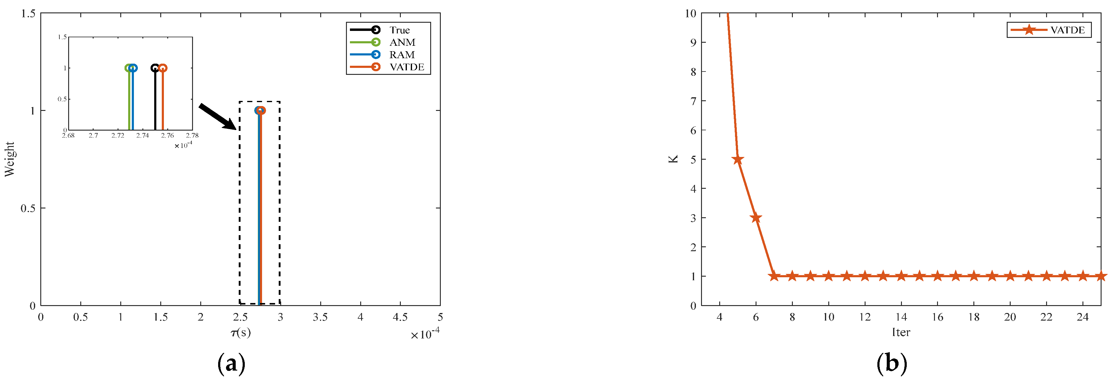
First, the ideal state was considered, that is, there was only one time delay between the received signals of the two sensors, the time delay value was $2.75\times {10}^{-4}$ s, and the normalized amplitude was 1. The signal-to-noise ratio (SNR) was set to 10 dB, and the end condition of the VATDE algorithm was ${{\Vert {\widehat{G}}_{x_1{x}_2}^{i-1}-{\widehat{G}}_{x_1{x}_2}^i\Vert }_2/\Vert {\widehat{G}}_{x_1{x}_2}^{i-1}\Vert }_2<{10}^{-6}$, then $i=3000$ represents the maximum number of iterations. Next, we compared the time delay estimation performance of the VATDE algorithm proposed in this paper with the ANM and RAM algorithms.

It can be seen from Figure 1a that all three algorithms, i.e., the ANM and RAM methods, and the VATDE proposed in this paper, could obtain better time delay estimation results in the case of a single time delay. Meanwhile, the enlarged window in Figure 1a further shows that the VATDE algorithm was closer to the real-time delay than the RAM and ANM algorithms. Therefore, the VATDE algorithm’s time delay estimation accuracy was higher, while the time delay estimation accuracy of the RAM algorithm was also slightly better than that of the ANM algorithm. Figure 1b shows the estimation of the number of time delays existing using the VATDE algorithm. However, since the ANM and RAM algorithms cannot provide an estimate of the number of time delays, the number of time delays can only be manually determined. It can be seen from Figure 1b that the VATDE algorithm provided an accurate estimation of the number of time delays with only a few simple iterations, which avoids the interference caused by false peaks when determining the true time delay estimation.

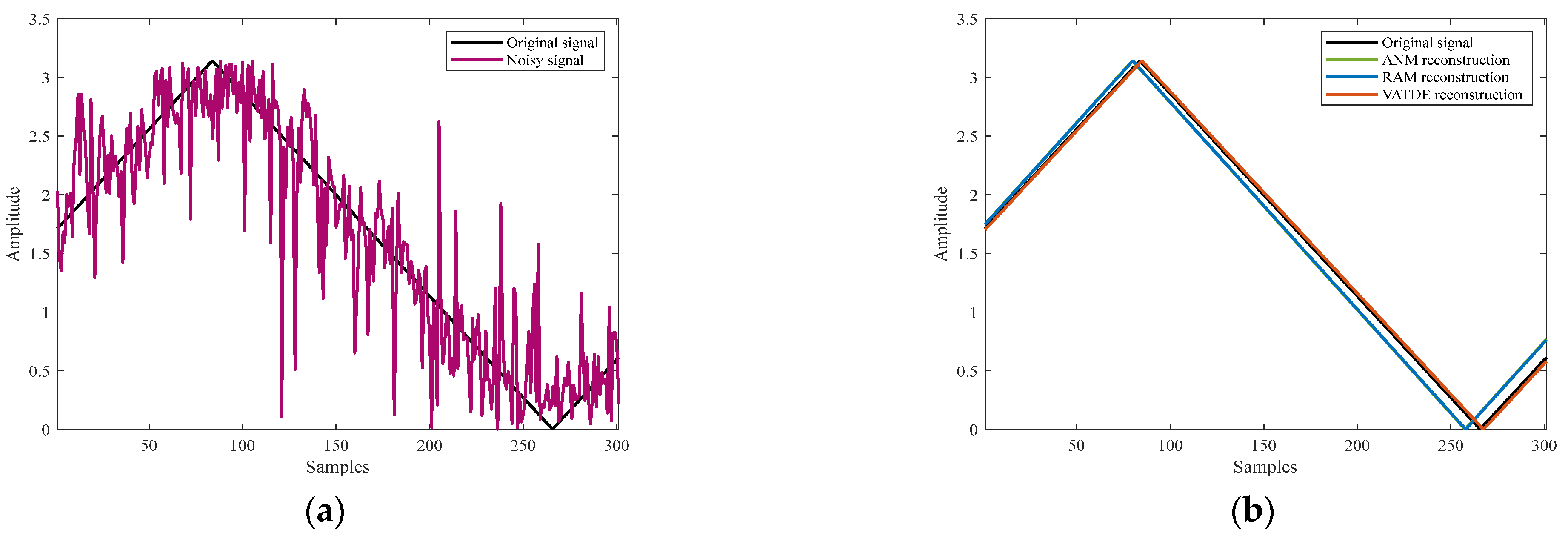
Figure 2a shows a comparison of the phase of the cross-power spectrum between the received signals in the case of no noise and the phase of the cross-power spectrum when the SNR was 10 dB. Figure 2b shows the performance of different algorithms for reconstructing the original cross-power spectrum phase from the noisy cross-power spectrum phase. It can be clearly seen that the reconstructed cross-power spectrum phase obtained by the proposed VATDE algorithm fitted the original cross-power spectrum phase perfectly. In addition, the reconstruction performance of the ANM algorithm was similar to that of the RAM algorithm. Although the trend of the reconstructed cross-power spectrum phase was roughly the same as that of the original cross-power spectrum phase, there was still a certain deviation. Clearly, the time delay estimation performance of the algorithm is was to the reconstruction performance of the cross-power spectrum. When the time delay estimation of the algorithm was more accurate, then the reconstructed cross-power spectrum phase becomes more suitable for the original cross-power spectrum phase.

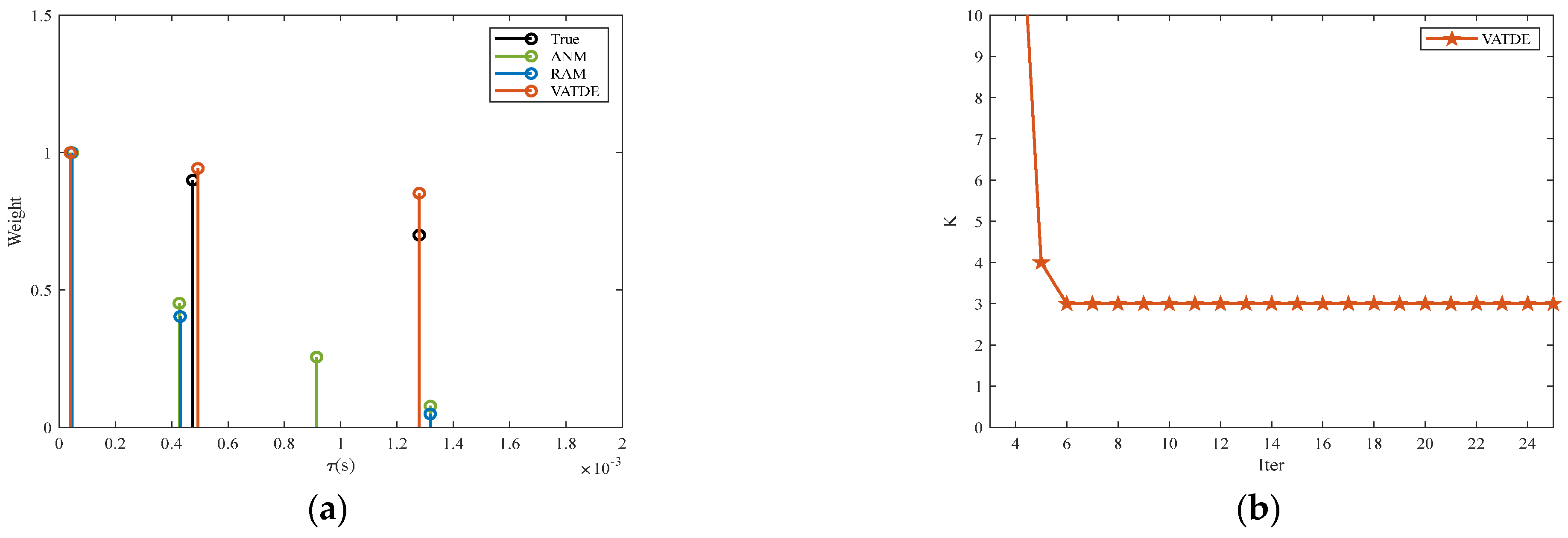
Second, assuming the presence of a multipath influence, there were two time delays between the received signals of the two sensors, which signifies that there will be three time delays in the cross-power spectrum. In this paper, the magnitudes of the three time delays were set to $[0.45\times {10}^{-4} \mathrm{s},4.75\times {10}^{-4} \mathrm{s},12.79\times {10}^{-4} \mathrm{s}]$, and the amplitudes were $[1,0.9,0.7]$, respectively, while the SNR was also set as 10 dB. This paper compared the time delay estimation performance of the VATDE algorithm proposed in this paper with those of the ANM and RAM algorithms.

Figure 3a shows the time delay estimation results of the VATDE, ANM, and RAM algorithms in the presence of three time delay values. It can be seen that, compared with the ANM and RAM algorithms, the VATDE algorithm not only provided a more accurate time delay estimation result, it also yielded a more accurate amplitude estimate. The time delay estimation results of the RAM algorithm were similar to those of the ANM algorithm. However, under the same parameter selection, the RAM algorithm had fewer false peaks than the ANM algorithm, which reduced the interference of false peaks to the time delay estimation results. Figure 3b once again shows the estimated performance of the VATDE algorithm for the number of time delays present. It still only took a few simple iterations to estimate the real number of time delays, which is very meaningful for time delay estimation, as it avoids the problem of distinguishing the real delay from the obtained time delay estimation results.

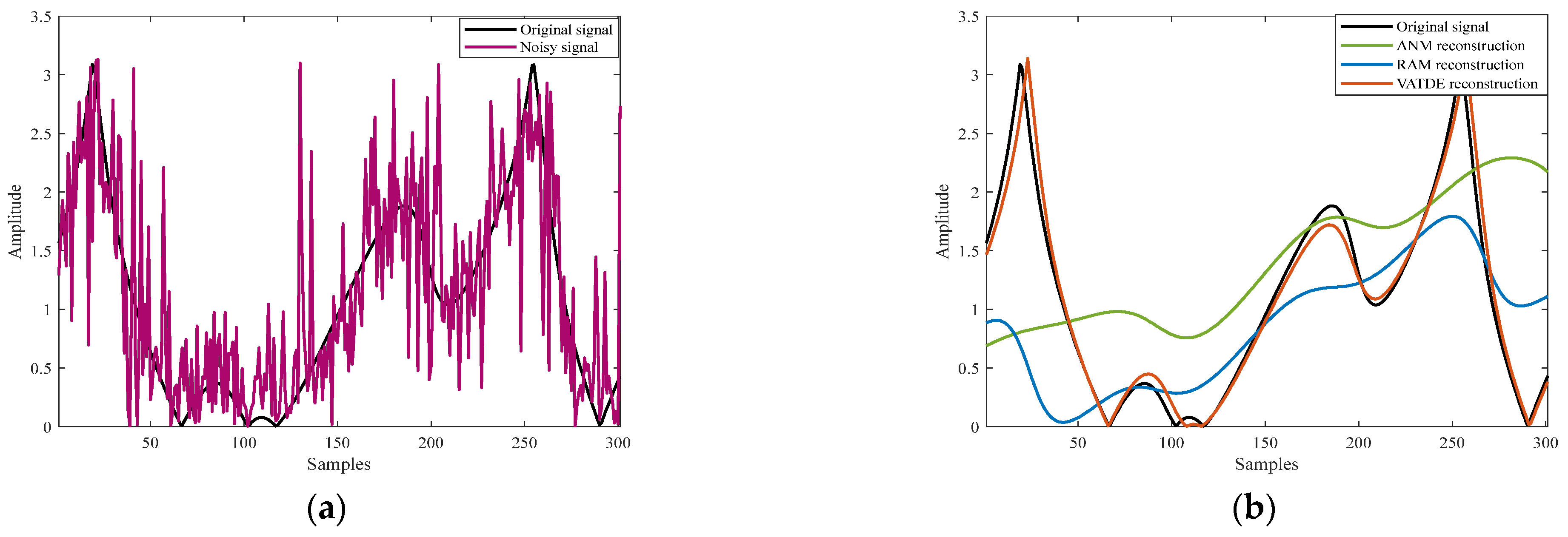
Figure 4a shows a comparison of the cross-power spectrum phase between the received signals in the case of no noise and the cross-power spectrum phase in the case of SNR 10 dB when there were three time delays. Compared with Figure 2a, the multiple time delays made the original cross-power spectrum phase more irregular; thus, it was more difficult to reconstruct the original cross-power spectrum phase from the noisy cross-power spectrum phase. Figure 4b shows the performance of different algorithms in reconstructing the original cross-power spectrum phase in the presence of three time delays. It is clear that the reconstructed cross-power spectrum phases of the ANM and RAM algorithms exhibited significant deviations from the original cross-power spectrum phase, due to their inaccurate time delay estimation and poor time delay amplitude estimation. Compared with the ANM algorithm, the reconstructed cross-power spectrum phase of the RAM algorithm could still reflect the original cross-power spectrum phase trend to a certain extent. This was because the reconstructed results of the ANM algorithm were greatly influenced by false peaks, and, thus, could not reflect the general trend of the original cross-power spectrum phase. Compared with the ANM and RAM algorithms, the reconstructed cross-power spectrum phase of the VATDE algorithm proposed in this paper still perfectly fitted the original cross-power spectrum phase, which once again reflects the superiority of the VATDE algorithm.

Next, the computational efficiency of the different algorithms was compared. In this study, 100 Monte Carlo simulations were carried out under the multipath assumption. The ANM and RAM algorithms in this paper were solved using the SDPT3 [26] solver in the CVX toolbox [27]. Based on reference [28], the time complexity of the CVX toolbox for solving the semi-positive definite problem was approximately $\mathrm{O}(N^3)$ Thus, the time complexity of ANM was approximately $\mathrm{O}(N^3)$. Since the estimation result of the RAM algorithm was obtained using multiple iterations of the ANM algorithm, the time complexity of RAM was approximately $\mathrm{O}(L{N}^3)$, where $L$ denotes the number of iterations. The time complexity of VATDE was approximately $\mathrm{O}(N^2)$. Obviously, VATDE was the most computationally efficient in theory.

The average running times of the ANM, RAM, and VATDE algorithms in MATLAB 2020a are shown in

Table 1. RUNNING TIME (INTEL^R CORE^TM i7-10510U CPU @ 1.80 GHz).

Algorithm	ANM	RAM	VATDE
Times (s)	148.1816	444.5448	7.8203

. Compared with the ANM and RAM algorithms, VATDE clearly had the shortest running time. The running times of the ANM and RAM algorithms were much longer than that of the VATDE algorithm. The running time of the RAM algorithm was a multiple of the running time of the ANM algorithm, and the specific value depended on the number of iterations. In this paper, the number of iterations was set to three and it can be seen that RAM took three times as long as ANM to complete. The simulation results were consistent with the theory and prove the high computational efficiency of the VATDE algorithm.

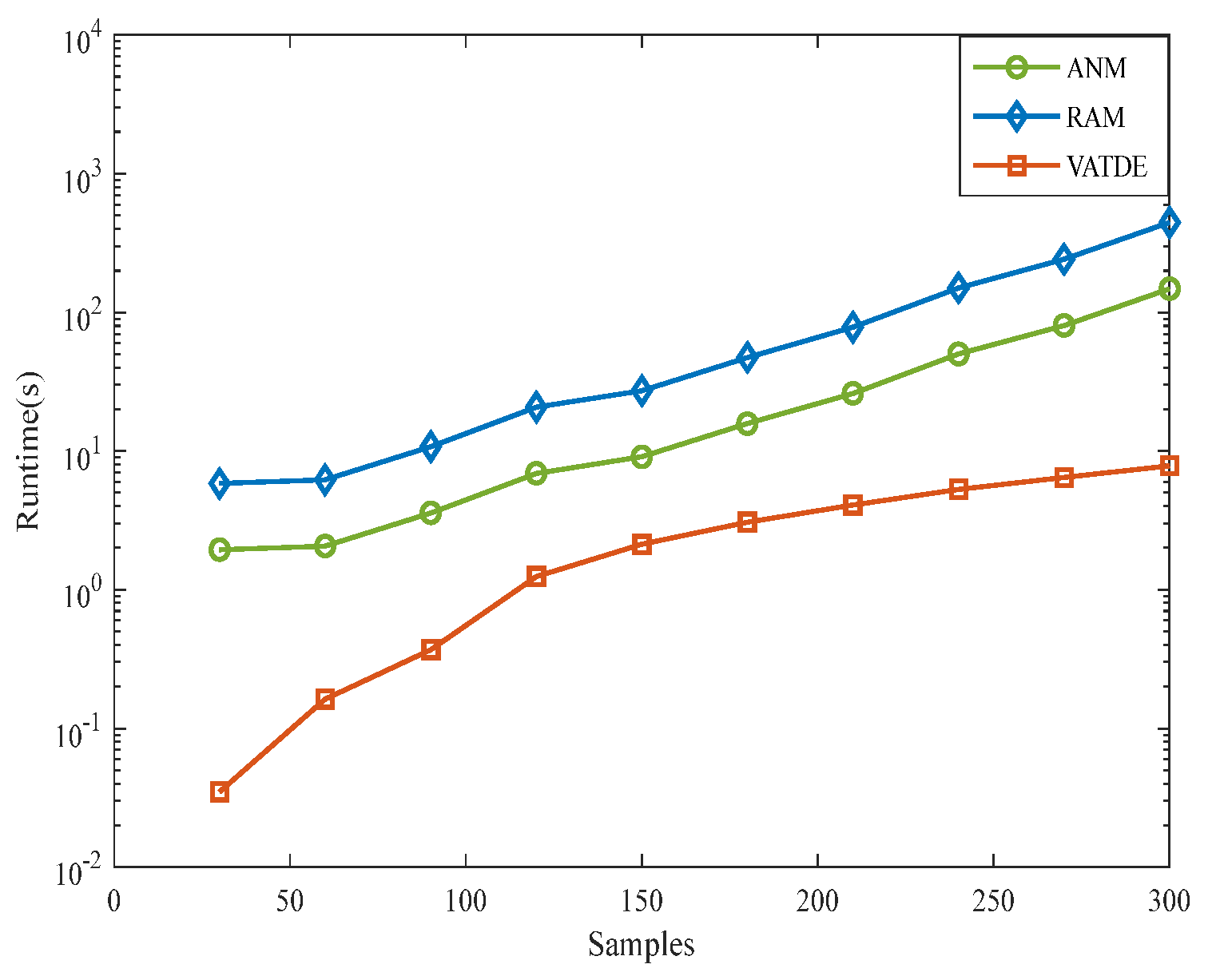
Of course, for the ANM, RAM, and VATDE algorithms, the running time was affected by the number of sampling points. When the number of sampling points is higher, the running time will be longer. However, as shown by the results in Figure 5, when the number of sampling point varied from 30 to 300, the running time and sampling points did not change linearly, and the multiplier of the increase in running time was greater than the multiplier of the increase in sampling points. Therefore, when the running time is long due to a large number of sampling points, the calculation efficiency can be improved by dividing the dataset into multiple small sets of sampling points. In addition, the results in Figure 5 show that the VALSE algorithm possessed computational advantages compared with the ANM and RAM algorithms at different numbers of sampling points, and the computational efficiency was more than 10 times that of the ANM algorithm.

Based on the above calculation efficiency comparison, it can be concluded that the VATDE algorithm proposed in this paper is more likely to be applied to real-time data processing.

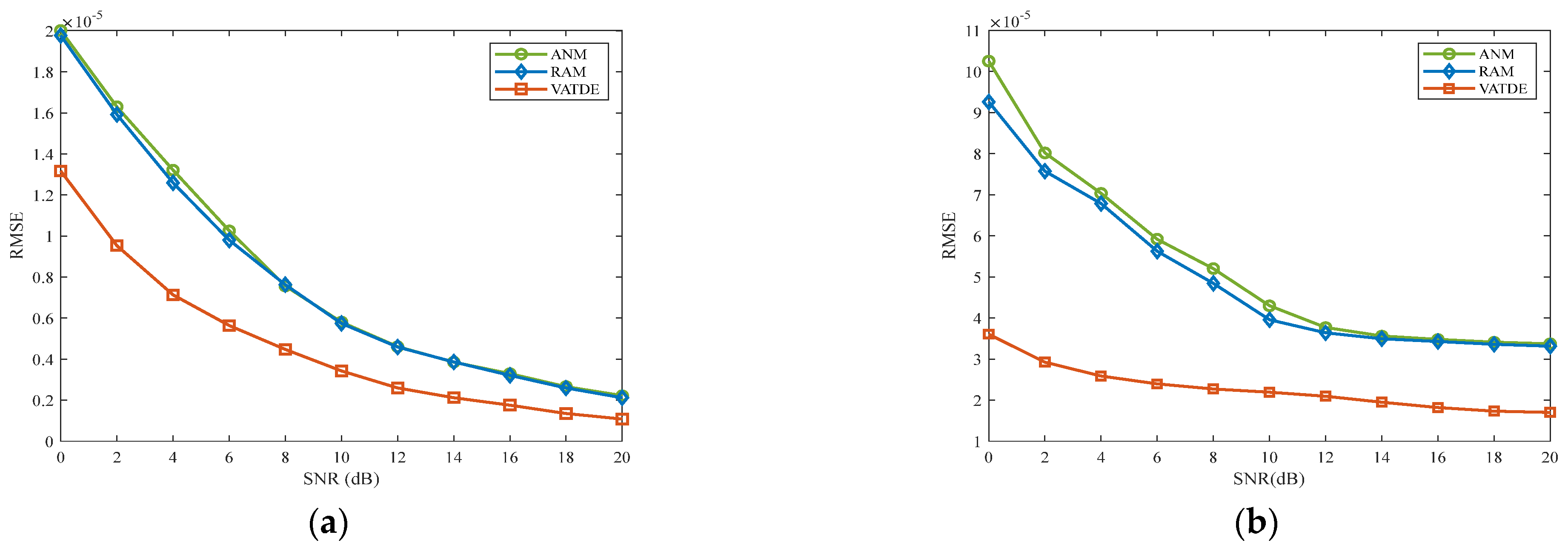
Finally, the root-mean-squared error (RMSE) and SNR curves were plotted to show the time delay estimation accuracy of the three algorithms. Considering the different uses of time delay estimation, this paper divided the accuracy of delay estimation into two categories. One is the time delay estimation accuracy in the case of a single time delay without considering the multipath effect, which is usually applied to the geometric positioning problem in passive sonars [9]. The second category is the time delay estimation accuracy with multiple time delays in the multipath environment. The multipath effect will lead to more than three peaks in the cross-correlation function. The depth estimation problem of underwater targets can be solved by estimating multiple time delays [10].

Meanwhile, the signal simulation remained unchanged. The settings of single time delay and multiple time delays were the same as those in the above simulation. When SNR changed from 0 dB to 20 dB, then the RMSE of the ANM, RAM, and VATDE algorithms was compared, and each result was obtained using 500 Monte Carlo simulations. The simulation results are shown in Figure 6. Figure 6a shows the RMSE and SNR curves under a single time delay, while Figure 6b shows the RMSE and SNR curves under multiple time delays. It can be seen that the RMSE of the VATDE algorithm was lower than that of the ANM and RAM algorithms in the cases of both single and multiple time delays. Especially in a low SNR environment, the time delay estimation accuracy of the ANM and RAM algorithms deteriorated significantly, while VATDE still had high time delay estimation accuracy. In addition, the RMSE of the ANM and RAM algorithms was approximately equal with a single time delay, but with multiple time delays, the RMSE of the RAM algorithm was lower than that of the ANM algorithm. This may be because the RAM algorithm had fewer false peaks than the ANM algorithm. Moreover, it can be seen from the RMSE results in Figure 6a,b that the RMSE curves of the ANM, RAM, and VATDE algorithms in Figure 6b were much more than three times those in Figure 6a, which may have been due to the mutual interference between multiple time delays, which reduced the accuracy of time delay estimation. If the post-processing method of the cross-correlation function is adopted, that is, only the peak region of the cross-correlation function is searched separately, avoiding the search of the whole continuous time region, then the accuracy of time delay estimation with multiple time delays may be further improved. This is the next step of this study, and will not be discussed here.

5. Conclusions

In this paper, a time delay estimation algorithm based on variational Bayesian inference was proposed. All parameters in this algorithm were obtained by approximating its posterior probability distribution through variational Bayesian inference. Therefore, the advantages of the algorithm in this paper are that, firstly, it does not require any parameter adjustment and avoids the delay estimation error caused by improper parameter selection. Secondly, the algorithm presented in this paper is a grid-less time delay estimation method, which avoids the problem of mismatch between the grid and the real-time delay, and breaks the limitation of sampling rate, so that a time delay of arbitrary size can be estimated. Thirdly, the performance of the delay estimation was significantly improved by accounting for the uncertainty of the time delay estimation rather than calculating only the point estimate. Finally, the simulation results showed that, even compared with other current state-of-the-art grid-less time delay estimation methods, the proposed algorithm had higher time delay estimation accuracy in the case of a single time delay and multiple time delays. In particular, in a low SNR environment, the time delay results could still be accurately estimated, which makes it suitable for passive sonar signal processing.

As an outlook, the next research direction following on from this paper is to find a better variational approximation to improve the performance of the algorithm, especially in situations where the time delays are very closely spaced. Moreover, this paper hopes to further improve the computational efficiency of the algorithm for use in large-scale scenarios.