
Multi-Target Tracking in Multi-Static Networks with Autonomous Underwater Vehicles Using a Robust Multi-Sensor Labeled Multi-Bernoulli Filter
 , and
, and
Abstract
:1. Introduction
2. Background and Objective
2.1. Multi-Target State and LMB RFS
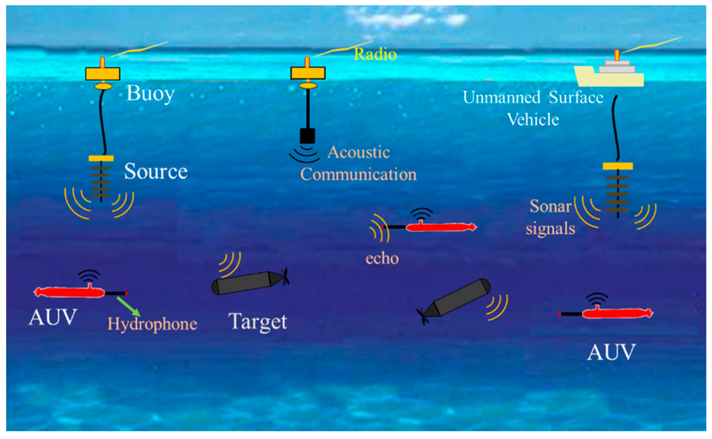
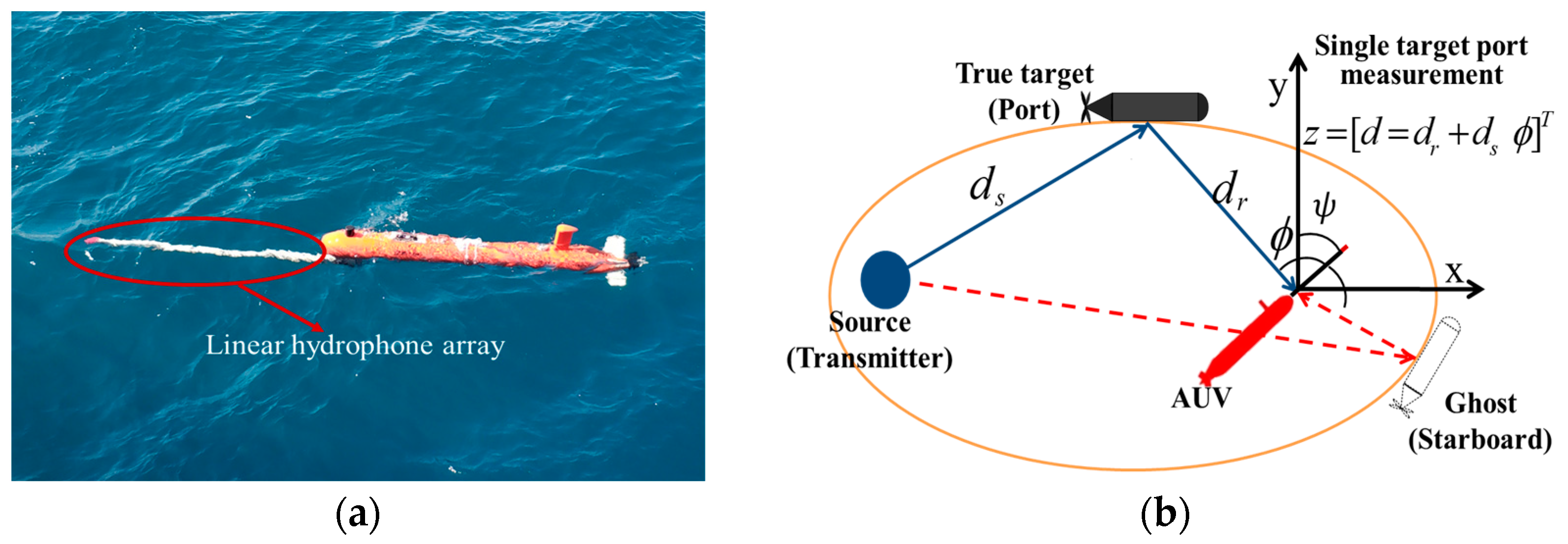
2.2. Measurement Model
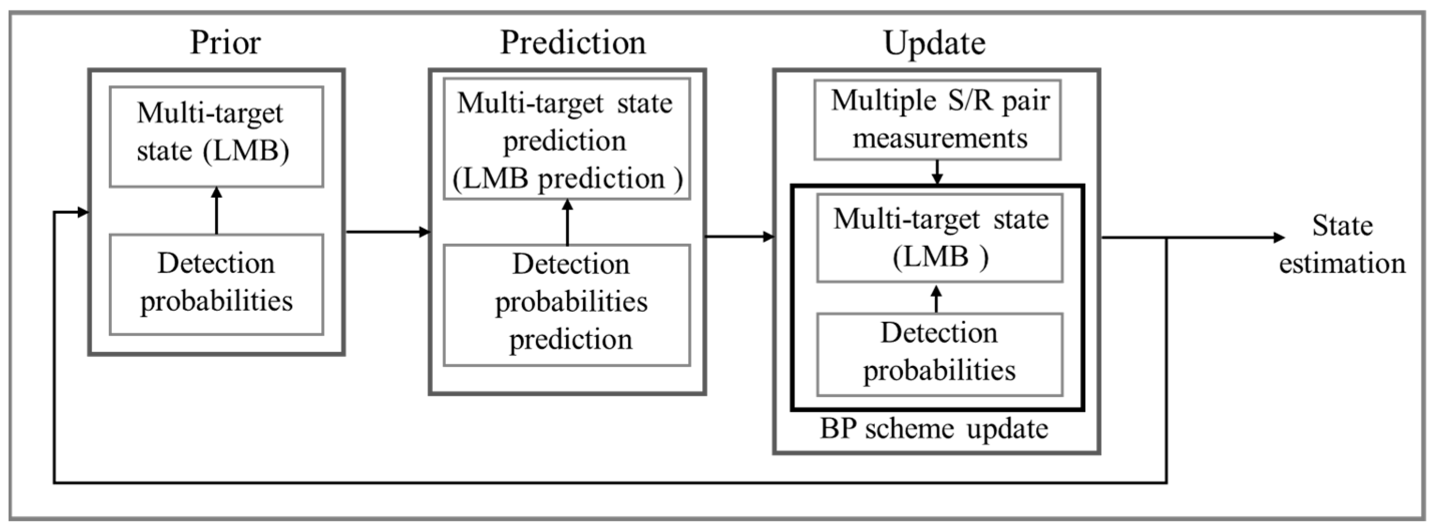
2.3. Multi-Sensor LMB Filter
2.4. Inference Objective
3. R-MS-LMB Model and the LMB Approximation
3.1. Robust Multi-Sensor LMB Model
3.2. LMB Approximation
4. The BP-Based Framework of the R-MS-LMB Filter
4.1. Joint Posterior Distributions
4.2. Factorization of the Joint Posterior Distribution
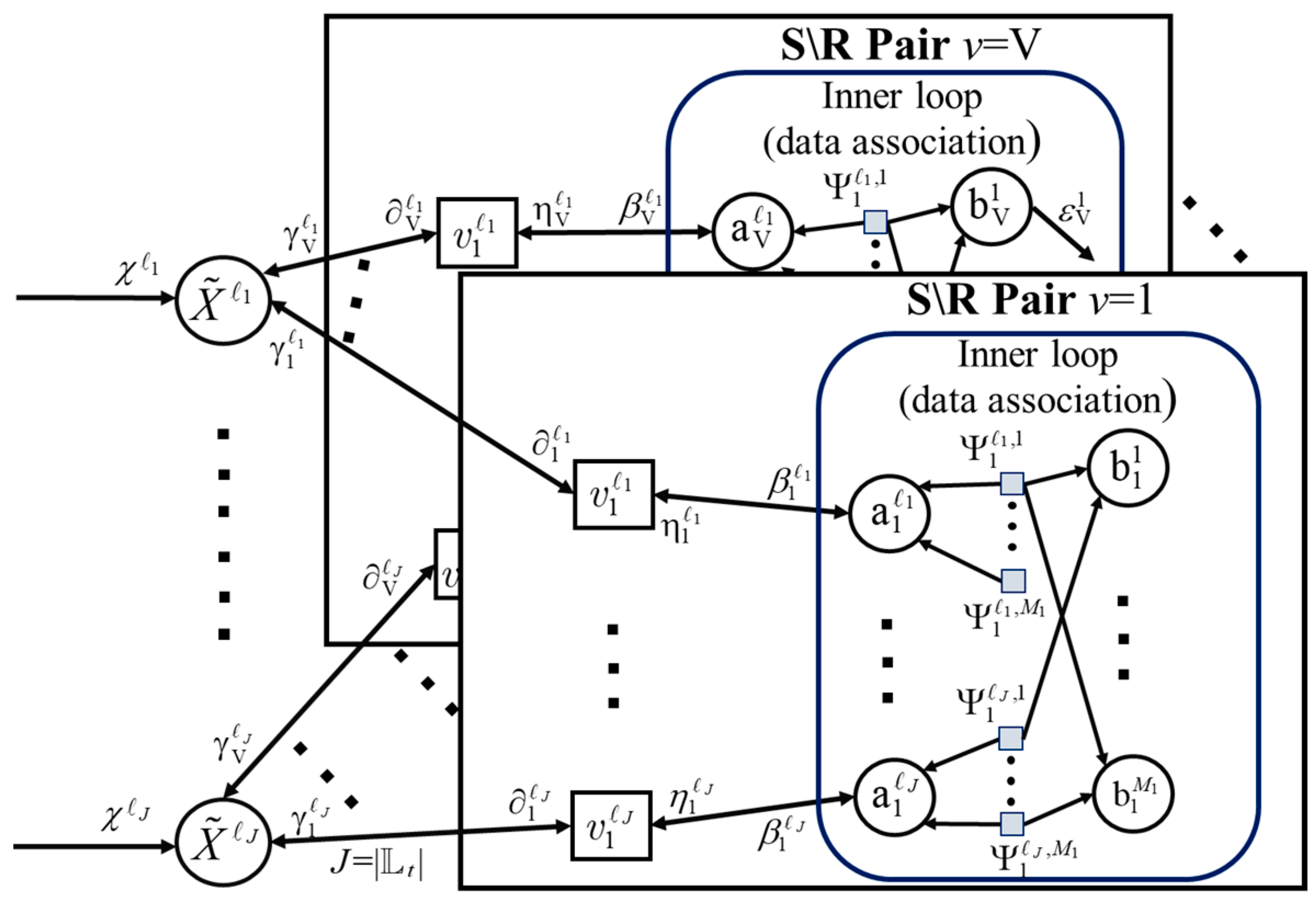
4.3. BP Scheme
4.4. Implementation
- (1)
- The augmented state of the PT for newly birthed LMB is a GB form:where , , , and are the given parameters.
- (2)
- The kinematic model for the single PT is an acceleration model [3]:
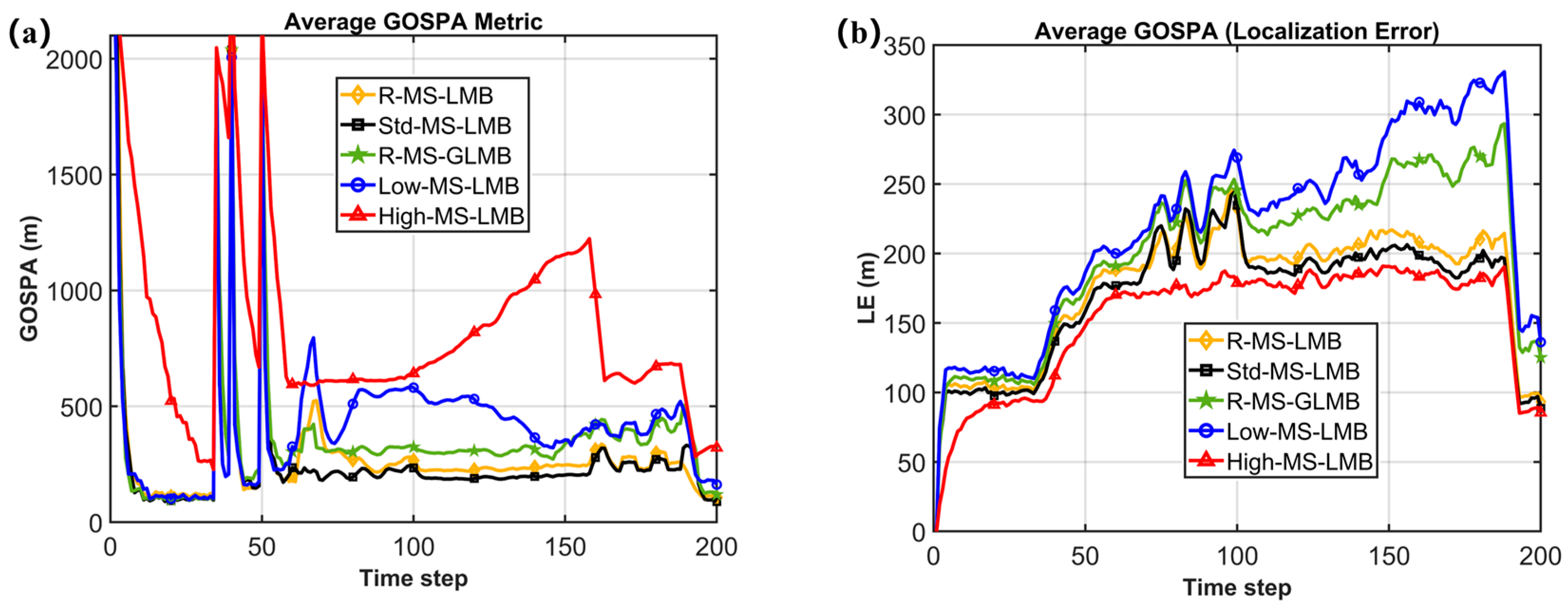
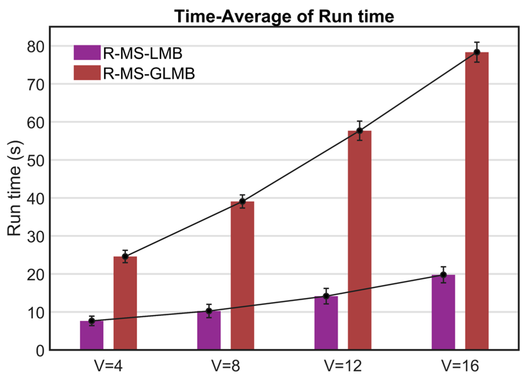
5. Numerical Study
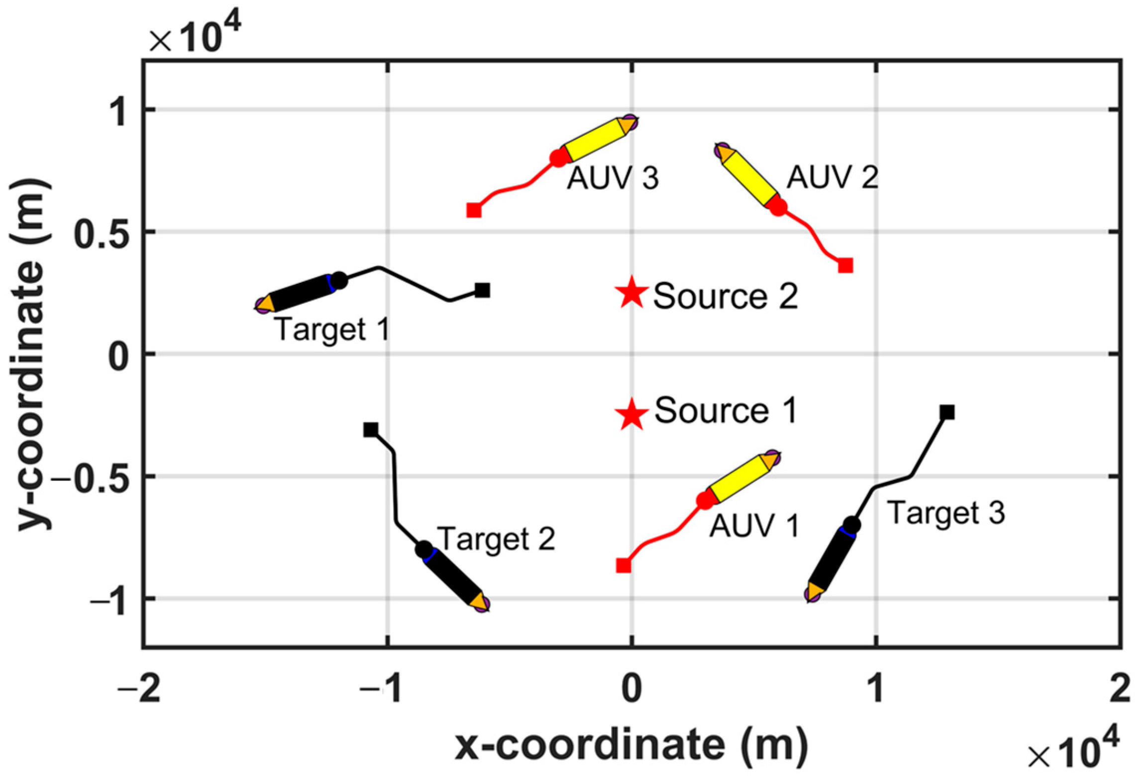
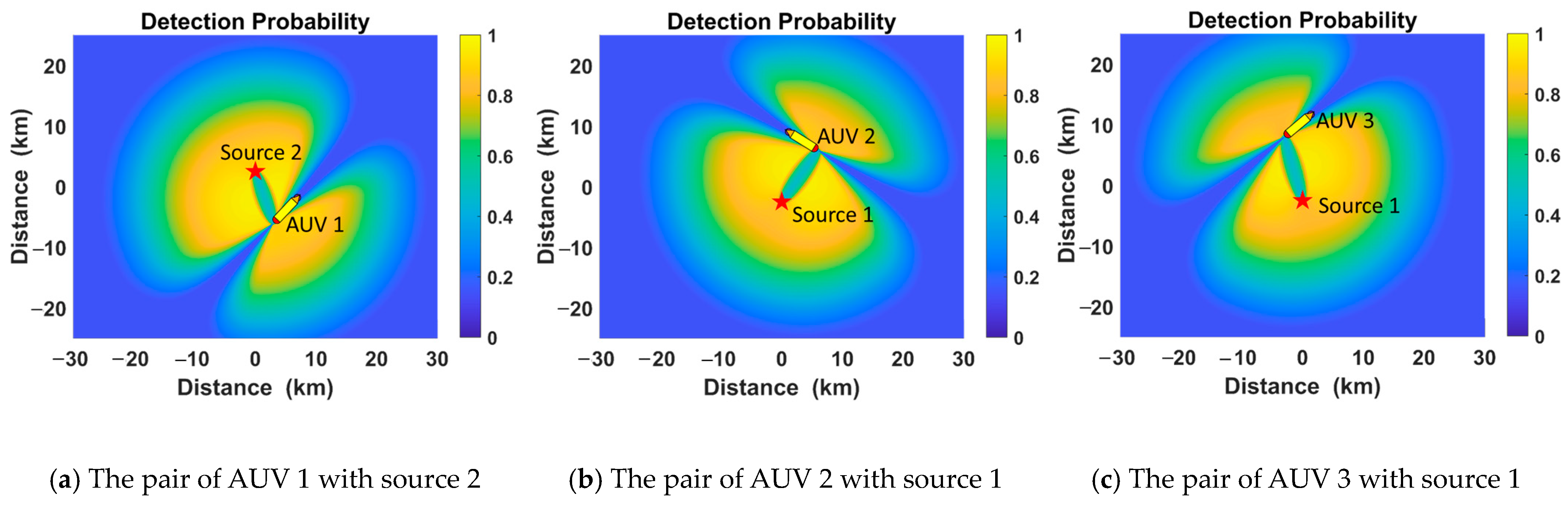
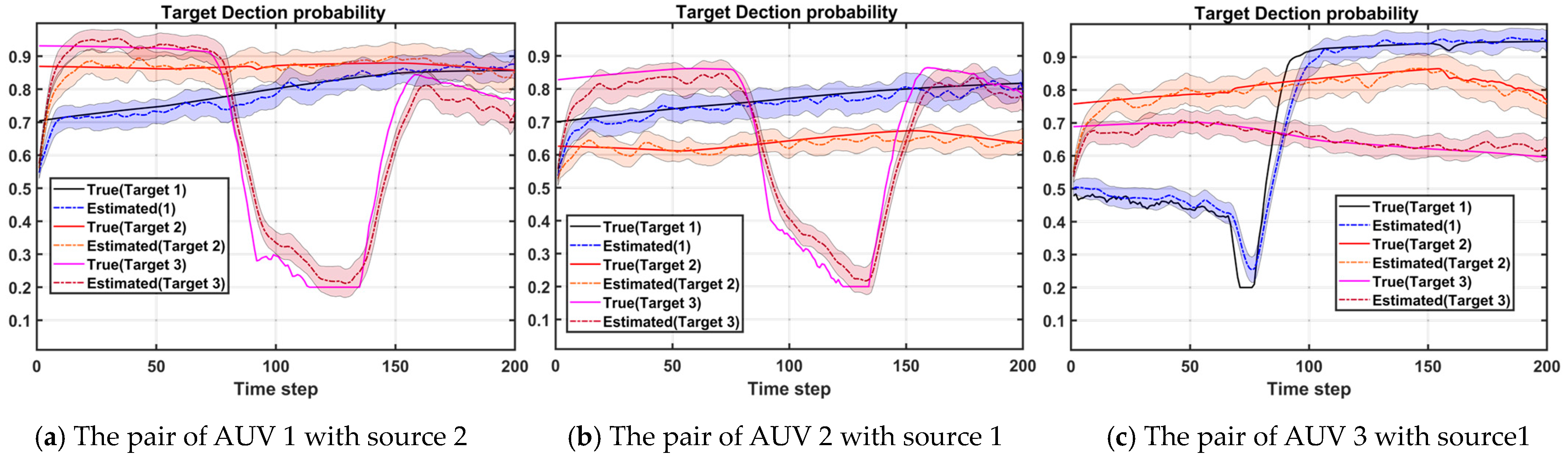
5.1. First Scenario
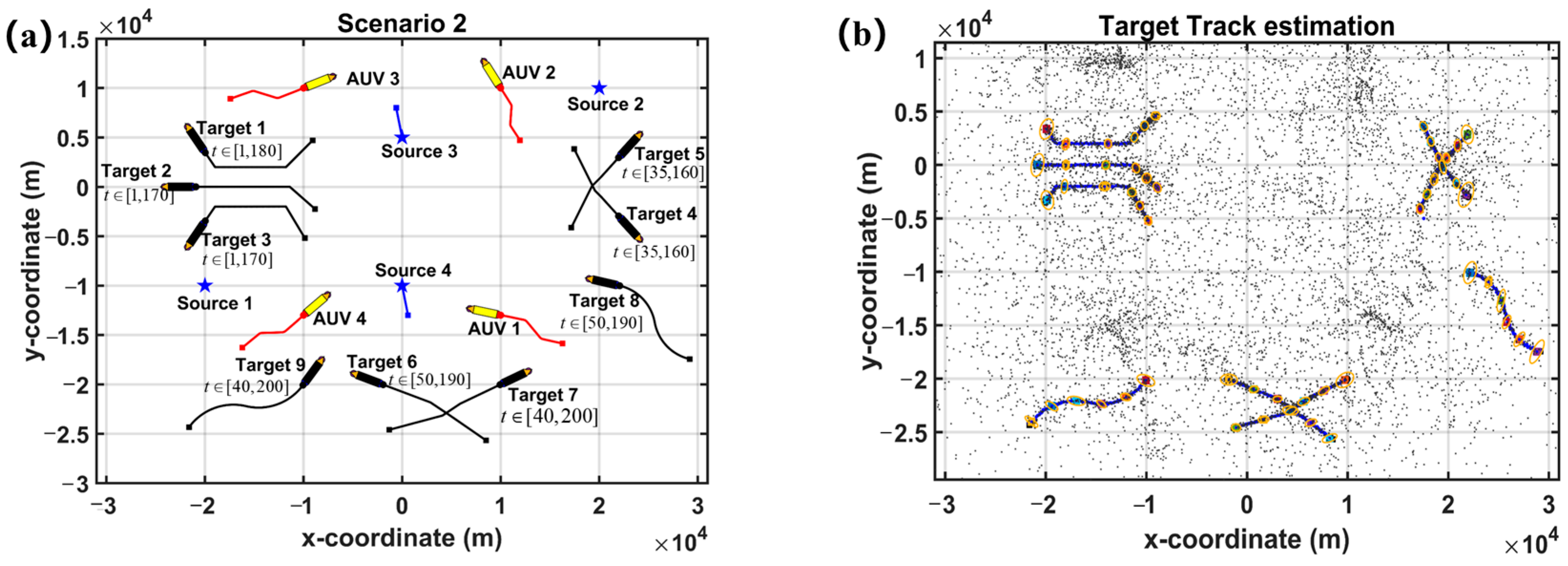
5.2. Second Scenario
6. Conclusions
Author Contributions
Funding
Institutional Review Board Statement
Informed Consent Statement
Data Availability Statement
Conflicts of Interest
References
- Luo, J.H.; Han, Y.; Fan, L.Y. Underwater Acoustic Target Tracking: A Review. Sensors 2018, 18, 112. [Google Scholar] [CrossRef] [PubMed]
- Kumar, M.; Mondal, S. Recent developments on target tracking problems: A review. Ocean Eng. 2021, 236, 109558. [Google Scholar] [CrossRef]
- Bar-Shalom, Y.; Li, X.R.; Kirubarajan, T. Tracking and Data Fusion: A Handbook of Algorithms; Academic Press: San Diego, CA, USA, 2011. [Google Scholar]
- Liu, Y.; Wang, M.; Su, Z.; Luo, J.; Xie, S.; Peng, Y.; Pu, H.; Xie, J.; Zhou, R. Multi-auvs cooperative target search based on autonomous cooperative search learning algorithm. J. Mar. Sci. Eng. 2020, 8, 843. [Google Scholar] [CrossRef]
- Xie, Y.; Song, T.L. Bearings-only multi-target tracking using an improved labeled multi-Bernoulli filter. Signal Process. 2018, 151, 32–44. [Google Scholar] [CrossRef]
- Wang, Y.; Wang, H.; Li, Q.; Xiao, Y.; Ban, X. Passive Sonar Target Tracking Based on Deep Learning. J. Mar. Sci. Eng. 2022, 10, 181. [Google Scholar] [CrossRef]
- Awan, K.M.; Shah, P.A.; Iqbal, K.; Gillani, S.; Ahmad, W.; Nam, Y. Underwater Wireless Sensor Networks: A Review of Recent Issues and Challenges. Wirel. Commun. Mob. Comput. 2019, 2019, 6470359. [Google Scholar] [CrossRef]
- Ferri, G.; Munafo, A.; Tesei, A.; Braca, P.; Meyer, F.; Pelekanakis, K.; Petroccia, R.; Alves, J.; Strode, C.; LePage, K. Cooperative robotic networks for underwater surveillance: An overview. IET Radar Sonar Navig. 2017, 11, 1740–1761. [Google Scholar] [CrossRef]
- Munafo, A.; Canepa, G.; LePage, K.D. Continuous Active Sonars for Littoral Undersea Surveillance. IEEE J. Ocean. Eng. 2019, 44, 1198–1212. [Google Scholar] [CrossRef]
- Ferri, G.; Petroccia, R.; De Magistris, G.; Morlando, L.; Micheli, M.; Tesei, A.; LePage, K. Cooperative Autonomy in the CMRE ASW Multistatic Robotic Network: Results From LCAS18 Trial. In Proceedings of the OCEANS—Marseille Conference, Marseille, France, 17–20 June 2019. [Google Scholar]
- Braca, P.; Goldhahn, R.; Ferri, G.; LePage, K.D. Distributed Information Fusion in Multistatic Sensor Networks for Underwater Surveillance. IEEE Sens. J. 2016, 16, 4003–4014. [Google Scholar] [CrossRef]
- Sahoo, A.; Dwivedy, S.K.; Robi, P.S. Advancements in the field of autonomous underwater vehicle. Ocean Eng. 2019, 181, 145–160. [Google Scholar] [CrossRef]
- Liu, H.; Xu, B.; Liu, B. A Tracking Algorithm for Sparse and Dynamic Underwater Sensor Networks. J. Mar. Sci. Eng. 2022, 10, 337. [Google Scholar] [CrossRef]
- Mohsan, S.A.H.; Li, Y.; Sadiq, M.; Liang, J.; Khan, M.A. Recent Advances, Future Trends, Applications and Challenges of Internet of Underwater Things (IoUT): A Comprehensive Review. J. Mar. Sci. Eng. 2023, 11, 124. [Google Scholar] [CrossRef]
- Braca, P.; Goldhahn, R.; LePage, K.D.; Marano, S.; Matta, V.; Willett, P. Cognitive Multistatic AUV Networks. In Proceedings of the 17th International Conference on Information Fusion (FUSION), Salamanca, Spain, 7–10 July 2014. [Google Scholar]
- Wolek, A.; McMahon, J.; Dzikowicz, B.R.; Houston, B.H. Tracking Multiple Surface Vessels With an Autonomous Underwater Vehicle: Field Results. IEEE J. Ocean. Eng. 2022, 47, 32–45. [Google Scholar] [CrossRef]
- Chong, C.-Y.; Mori, S.; Reid, D.B. Forty Years of Multiple Hypothesis Tracking—A Review of Key Developments. In Proceedings of the 21st International Conference on Information Fusion (FUSION), Cambridge, UK, 10–13 July 2018. [Google Scholar]
- Fortmann, T.E.; Barshalom, Y.; Scheffe, M. Sonar tracking of multiple targets using joint probabilistic data association. IEEE J. Ocean. Eng. 1983, 8, 173–184. [Google Scholar] [CrossRef]
- Musicki, D.; Evans, R. Joint integrated probabilistic data association: JIPDA. IEEE Trans. Aerosp. Electron. Syst. 2004, 40, 1093–1099. [Google Scholar] [CrossRef]
- Challa, S.; Morelande, M.R.; Mušicki, D.; Evans, R.J. Fundamentals of Object Tracking; Cambridge University Press: Cambridge, UK, 2011. [Google Scholar]
- Musicki, D.; Evans, R.J. Multiscan multitarget tracking in clutter with integrated track splitting filter. IEEE Trans. Aerosp. Electron. Syst. 2009, 45, 1432–1447. [Google Scholar] [CrossRef]
- Ronald, P.S. Advances in Statistical Multisource-Multitarget Information Fusion; Springer: New York, NY, USA, 2014. [Google Scholar]
- Mahler, R.; Ebrary, I. Statistical Multisource-Multitarget Information Fusion; Artech House: Norwood, MA, USA, 2007. [Google Scholar]
- Mahler, R.P.S. Multitarget Bayes filtering via first-order multitarget moments. IEEE Trans. Aerosp. Electron. Syst. 2003, 39, 1152–1178. [Google Scholar] [CrossRef]
- Mahler, R. PHD filters of higher order in target number. IEEE Trans. Aerosp. Electron. Syst. 2007, 43, 1523–1543. [Google Scholar] [CrossRef]
- Vo, B.T.; Vo, B.N.; Cantoni, A. The Cardinality Balanced Multi-Target Multi-Bernoulli Filter and Its Implementations. IEEE Trans. Signal Process. 2009, 57, 409–423. [Google Scholar] [CrossRef]
- Vo, B.N.; Vo, B.T.; Phung, D. Labeled Random Finite Sets and the Bayes Multi-Target Tracking Filter. IEEE Trans. Signal Process. 2014, 62, 6554–6567. [Google Scholar] [CrossRef]
- Reuter, S.; Vo, B.T.; Vo, B.N.; Dietmayer, K. The Labeled Multi-Bernoulli Filter. IEEE Trans. Signal Process. 2014, 62, 3246–3260. [Google Scholar] [CrossRef]
- Da, K.; Li, T.C.; Zhu, Y.F.; Fan, H.Q.; Fu, Q. Recent advances in multisensor multitarget tracking using random finite set. Front. Inf. Technol. Electron. Eng. 2021, 22, 5–24. [Google Scholar] [CrossRef]
- Nannuru, S.; Blouin, S.; Coates, M.; Rabbat, M. Multisensor CPHD Filter. IEEE Trans. Aerosp. Electron. Syst. 2016, 52, 1834–1854. [Google Scholar] [CrossRef]
- Saucan, A.A.; Coates, M.J.; Rabbat, M. A Multisensor Multi-Bernoulli Filter. IEEE Trans. Signal Process. 2017, 65, 5495–5509. [Google Scholar] [CrossRef]
- Vo, B.N.; Vo, B.T.; Beard, M. Multi-Sensor Multi-Object Tracking With the Generalized Labeled Multi-Bernoulli Filter. IEEE Trans. Signal Process. 2019, 67, 5952–5967. [Google Scholar] [CrossRef]
- Goldhahn, R.; Braca, P.; LePage, K.D.; Willett, P.; Marano, S.; Matta, V. Environmentally sensitive particle filter tracking in mu tistatic auv networks with port-starboard ambiguity. In Proceedings of the IEEE International Conference on Acoustics, Speech and Signal Processing (ICASSP), Florence, Italy, 4–9 May 2014. [Google Scholar]
- Ferri, G.; Munafo, A.; LePage, K.D. An Autonomous Underwater Vehicle Data-Driven Control Strategy for Target Tracking. IEEE J. Ocean. Eng. 2018, 43, 323–343. [Google Scholar] [CrossRef]
- Georgescu, R.; Willett, P. The GM-CPHD Tracker Applied to Real and Realistic Multistatic Sonar Data Sets. IEEE J. Ocean. Eng. 2012, 37, 220–235. [Google Scholar] [CrossRef]
- Mahler, R.P.S.; Vo, B.T.; Vo, B.N. CPHD Filtering With Unknown Clutter Rate and Detection Profile. IEEE Trans. Signal Process. 2011, 59, 3497–3513. [Google Scholar] [CrossRef]
- Li, C.M.; Wang, W.G.; Kirubarajan, T.; Sun, J.P.; Lei, P. PHD and CPHD Filtering With Unknown Detection Probability. IEEE Trans. Signal Process. 2018, 66, 3784–3798. [Google Scholar] [CrossRef]
- Li, G.C.; Kong, L.J.; Yi, W.; Li, X.L. Robust Poisson Multi-Bernoulli Mixture Filter With Unknown Detection Probability. IEEE Trans. Veh. Technol. 2021, 70, 886–899. [Google Scholar] [CrossRef]
- Zhang, Z.G.; Li, Q.; Sun, J.P. Multisensor RFS Filters for Unknown and Changing Detection Probability. Electronics 2019, 8, 741. [Google Scholar] [CrossRef]
- Punchihewa, Y.G.; Vo, B.T.; Vo, B.N.; Kim, D.Y. Multiple Object Tracking in Unknown Backgrounds With Labeled Random Finite Sets. IEEE Trans. Signal Process. 2018, 66, 3040–3055. [Google Scholar] [CrossRef]
- Soldi, G.; Meyer, F.; Braca, P.; Hlawatsch, F. Self-Tuning Algorithms for Multisensor-Multitarget Tracking Using Belief Propagation. IEEE Trans. Signal Process. 2019, 67, 3922–3937. [Google Scholar] [CrossRef]
- Do, C.T.; Nguyen, T.T.D.; Nguyen, H.V. Robust multi-sensor generalized labeled multi-Bernoulli filter. Signal Process. 2022, 192, 108368. [Google Scholar] [CrossRef]
- Do, C.T.; Nguyen, T.T.D.; Liu, W.F. Tracking Multiple Marine Ships via Multiple Sensors with Unknown Backgrounds. Sensors 2019, 19, 5025. [Google Scholar] [CrossRef]
- Robertson, S.C.J.; van Daalen, C.E.; du Preez, J.A. Efficient approximations of the multi-sensor labelled multi-Bernoulli filter. Signal Process. 2022, 199, 108633. [Google Scholar] [CrossRef]
- Kropfreiter, T.; Meyer, F.; Hlawatsch, F. A Fast Labeled Multi-Bernoulli Filter Using Belief Propagation. IEEE Trans. Aerosp. Electron. Syst. 2020, 56, 2478–2488. [Google Scholar] [CrossRef]
- Vo, B.N.; Vo, B.T.; Pham, N.T.; Suter, D. Joint Detection and Estimation of Multiple Objects From Image Observations. IEEE Trans. Signal Process. 2010, 58, 5129–5141. [Google Scholar] [CrossRef]
- Grimmett, D.; Wakayama, C. Multistatic Tracking for Continous Active Sonar using Doppler-Bearing Measurements. In Proceedings of the 16th International Conference on Information Fusion (FUSION), Istanbul, Turkey, 9–12 July 2013. [Google Scholar]
- Coraluppi, S. Multistatic sonar localization. IEEE J. Ocean. Eng. 2006, 31, 964–974. [Google Scholar] [CrossRef]
- Braca, P.; Willett, P.; LePage, K.; Marano, S.; Matta, V. Bayesian Tracking in Underwater Wireless Sensor Networks With Port-Starboard Ambiguity. IEEE Trans. Signal Process. 2014, 62, 1864–1878. [Google Scholar] [CrossRef]
- Williams, J.; Lau, R. Approximate Evaluation of Marginal Association Probabilities With Belief Propagation. IEEE Trans. Aerosp. Electron. Syst. 2014, 50, 2942–2959. [Google Scholar] [CrossRef]
- Sharma, P.; Saucan, A.A.; Bucci, D.J.; Varshney, P.K. Decentralized Gaussian Filters for Cooperative Self-Localization and Multi-Target Tracking. IEEE Trans. Signal Process. 2019, 67, 5896–5911. [Google Scholar] [CrossRef]
- Meyer, F.; Kropfreiter, T.; Williams, J.L.; Lau, R.A.; Hlawatsch, F.; Braca, P.; Win, M.Z. Message Passing Algorithms for Scalable Multitarget Tracking. Proc. IEEE 2018, 106, 221–259. [Google Scholar] [CrossRef]
- Kschischang, F.R.; Frey, B.J.; Loeliger, H.A. Factor graphs and the sum-product algorithm. IEEE Trans. Inf. Theory 2001, 47, 498–519. [Google Scholar] [CrossRef]
- Yedidia, J.S.; Freeman, W.T.; Weiss, Y. Constructing free-energy approximations and generalized belief propagation algorithms. IEEE Trans. Inf. Theory 2005, 51, 2282–2312. [Google Scholar] [CrossRef]
- Meyer, F.; Braca, P.; Willett, P.; Hlawatsch, F. A Scalable Algorithm for Tracking an Unknown Number of Targets Using Multiple Sensors. IEEE Trans. Signal Process. 2017, 65, 3478–3493. [Google Scholar] [CrossRef]
- Williams, J.L.; Lau, R.A. Convergence of loopy belief propagation for data association. In Proceedings of the Sixth International Conference on Intelligent Sensors, Shanghai, China, 7–10 December 2011. [Google Scholar]
- Correa, J.; Adams, M. Estimating Detection Statistics within a Bayes-Closed Multi-Object Filter. In Proceedings of the 19th International Conference on Information Fusion (FUSION), Heidelberg, Germany, 5–8 July 2016. [Google Scholar]
- Ozer, E.; Hocaoglu, A.K. Robust Model-Dependent Poisson Multi Bernoulli Mixture Trackers for Multistatic Sonar Networks. IEEE Access 2021, 9, 163612–163624. [Google Scholar] [CrossRef]
- Rahmathullah, A.S.; Garcia-Fernandez, A.F.; Svensson, L. Generalized optimal sub-pattern assignment metric. In Proceedings of the 20th International Conference on Information Fusion (Fusion), Xi’an, China, 10–13 July 2017. [Google Scholar]


| Parameter | Value | Specification |
|---|---|---|
| T | 20 s | Time scan |
| 10−2 m/s2 | Process noise | |
| 100 m | Rang std. deviation | |
| 1° | Bearing std. deviation | |
| 0.95 | Prob. of survival | |
| 10−3 | Deleting threshold of PTs | |
| 10−3 | Extracting threshold of PTs | |
| b | 0.5 | Fermi function Para.b |
| 20 km | Fermi function Para.R0 | |
| 1.5 km | Fermi function Para.Rb | |
| 30° | End-fire angle | |
| 10 | False alarm rate |
| Filters | R-MS-LMB | R-MS-GLMB | Std-MS-LMB | Low-MS-LMB | High-MS-LMB |
|---|---|---|---|---|---|
| GOSPA (m) | 307.81 | 353.87 | 271.81 | 845.82 | 425.00 |
| LE (m) | 175.65 | 201.87 | 169.35 | 152.46 | 220.27 |
| ME (m) | 82.76 | 100.73 | 81.21 | 753.96 | 83.33 |
| FE (m) | 38.50 | 38.49 | 30.83 | 52.13 | 164.34 |
| Runtime (s) | 21.34 | 88.26 | 20.62 | 50.49 | 28.97 |
Disclaimer/Publisher’s Note: The statements, opinions and data contained in all publications are solely those of the individual author(s) and contributor(s) and not of MDPI and/or the editor(s). MDPI and/or the editor(s) disclaim responsibility for any injury to people or property resulting from any ideas, methods, instructions or products referred to in the content. |
© 2023 by the authors. Licensee MDPI, Basel, Switzerland. This article is an open access article distributed under the terms and conditions of the Creative Commons Attribution (CC BY) license (https://creativecommons.org/licenses/by/4.0/).
Share and Cite
Zhang, Y.; Li, Y.; Li, S.; Zeng, J.; Wang, Y.; Yan, S. Multi-Target Tracking in Multi-Static Networks with Autonomous Underwater Vehicles Using a Robust Multi-Sensor Labeled Multi-Bernoulli Filter. J. Mar. Sci. Eng. 2023, 11, 875. https://doi.org/10.3390/jmse11040875
Zhang Y, Li Y, Li S, Zeng J, Wang Y, Yan S. Multi-Target Tracking in Multi-Static Networks with Autonomous Underwater Vehicles Using a Robust Multi-Sensor Labeled Multi-Bernoulli Filter. Journal of Marine Science and Engineering. 2023; 11(4):875. https://doi.org/10.3390/jmse11040875
Chicago/Turabian StyleZhang, Yuexing, Yiping Li, Shuo Li, Junbao Zeng, Yiqun Wang, and Shuxue Yan. 2023. "Multi-Target Tracking in Multi-Static Networks with Autonomous Underwater Vehicles Using a Robust Multi-Sensor Labeled Multi-Bernoulli Filter" Journal of Marine Science and Engineering 11, no. 4: 875. https://doi.org/10.3390/jmse11040875